Do small and large floods have the same drivers of change? A regional attribution analysis in Europe
←
→
Page content transcription
If your browser does not render page correctly, please read the page content below

Hydrol. Earth Syst. Sci., 25, 1347–1364, 2021
https://doi.org/10.5194/hess-25-1347-2021
© Author(s) 2021. This work is distributed under
the Creative Commons Attribution 4.0 License.

Do small and large floods have the same drivers of change?
A regional attribution analysis in Europe
Miriam Bertola1 , Alberto Viglione2 , Sergiy Vorogushyn3 , David Lun1 , Bruno Merz3,4 , and Günter Blöschl1
1 Institute of Hydraulic Engineering and Water Resources Management, Vienna University of Technology,
Karlsplatz 13, 1040 Vienna, Austria
2 Department of Environment, Land and Infrastructure Engineering (DIATI), Polytechnic University of Turin,

Corso Duca degli Abruzzi 24, 10129 Turin, Italy
3 GFZ German Research Centre for Geosciences, Hydrology section, Telegrafenberg, 14473 Potsdam, Germany
4 Institute for Environmental Sciences and Geography, University of Potsdam, Karl-Liebknecht-Straße 24–25,

14476 Potsdam, Germany

Correspondence: Miriam Bertola (bertola@hydro.tuwien.ac.at)

Received: 1 August 2020 – Discussion started: 18 August 2020
Revised: 5 January 2021 – Accepted: 27 January 2021 – Published: 19 March 2021

Abstract. Recent studies have shown evidence of increas-           of antecedent soil moisture are of secondary importance. In
ing and decreasing trends for average floods and flood quan-       southern Europe, both antecedent soil moisture and extreme
tiles across Europe. Studies attributing observed changes in       precipitation contribute to flood changes, and their relative
flood peaks to their drivers have mostly focused on the aver-      importance depends on the return period. Antecedent soil
age flood behaviour, without distinguishing small and large        moisture is the main contributor to changes in q2 , while the
floods. This paper proposes a new framework for attributing        contributions of the two drivers to changes in larger floods
flood changes to potential drivers, as a function of return pe-    (T > 10 years) are comparable. In eastern Europe, snowmelt
riod (T ), in a regional context. We assume flood peaks to         drives changes in both q2 and q100 .
follow a non-stationary regional Gumbel distribution, where
the median flood and the 100-year growth factor are used as
parameters. They are allowed to vary in time and between
catchments as a function of the drivers quantified by covari-      1   Introduction
ates. The elasticities of floods with respect to the drivers and
the contributions of the drivers to flood changes are esti-        There is widespread concern that river flooding has become
mated by Bayesian inference. The prior distributions of the        more frequent and severe during the last decades and that
elasticities of flood quantiles to the drivers are estimated by    human-induced climate change and other drivers will fur-
hydrological reasoning and from the literature. The attribu-       ther increase flood discharge and damage in many parts of
tion model is applied to European flood and covariate data         the world (IPCC, 2012; Hirabayashi et al., 2013). This con-
and aims at attributing the observed flood trend patterns to       cern has given rise to a large number of studies investigat-
specific drivers for different return periods at the regional      ing past changes in flood hazard, i.e. changes related to flood
scale. We analyse flood discharge records from 2370 hydro-         discharge, and flood risk, i.e. changes related to damage. The
metric stations in Europe over the period 1960–2010. Ex-           global pattern of increasing flood damage has been mainly at-
treme precipitation, antecedent soil moisture and snowmelt         tributed to increasing population, economic activities and as-
are the potential drivers of flood change considered in this       sets in flood-prone areas (Bouwer, 2011; IPCC, 2012; Visser
study. Results show that, in northwestern Europe, extreme          et al., 2014). In terms of changes in flood discharge, a vari-
precipitation mainly contributes to changes in both the me-        ety of changes has been found (for shift in timing and trends
dian (q2 ) and 100-year flood (q100 ), while the contributions     in the magnitude of European floods, see Blöschl et al.,
                                                                   2017, 2019), and attempts to attribute detected changes have

Published by Copernicus Publications on behalf of the European Geosciences Union.
1348                                                               M. Bertola et al.: Regional attribution analysis in Europe

not resulted in a clear picture about the contribution of the      increasing variability of precipitation along with increasing
underlying drivers (for a review on detecting and attributing      mean in seasons other than summer, which leads to a dis-
flood hazard changes in Europe, see Hall et al., 2014).            proportional increase of heavy precipitation. Van den Besse-
   The large majority of studies on past changes in flood          laar et al. (2013) detected a decrease of the return period of
hazard analysed the mean flood behaviour, using, for in-           extreme precipitation (5, 10 and 20 years) over Europe in
stance, the Mann–Kendall test to detect gradual changes or         the past 60 years between 2 % and 58 %. Berg et al. (2013)
the Pettitt test for step changes in the mean or median annual     found a disproportional increase of high-intensity, convec-
flood (e.g. Petrow and Merz, 2009; Villarini et al., 2011; Me-     tive precipitation with increasing temperature that goes be-
diero et al., 2014; Mangini et al., 2018). They implicitly as-     yond the Clausius–Clapeyron rate (7 % per degree of tem-
sumed similar changes in different flood quantiles. This fo-       perature increase) compared to low-intensity, stratiform pre-
cus may be misleading, since changes in large floods may           cipitation. The review of a number of regional studies on past
differ from those in the average behaviour. An illustrative        precipitation trends in Europe by Madsen et al. (2014) sug-
example is the Mekong River, where studies found nega-             gested a tendency for increasing extreme rainfalls. This trend
tive trends in the mean flood discharge, whereas the public        seemed not to translate directly into positive trends in ob-
perception suggested that the frequency of damaging floods         served streamflow over large scales in Europe (Madsen et al.,
had increased in the past decades. Delgado et al. (2010) re-       2014). Similarly, Hodgkins et al. (2017) suggested that oc-
solved this mismatch by analysing the temporal change in           currence of floods with return periods of 25 to 100 years is
flood discharge variability. They found an upward trend in in-     dominated by multi-decadal climate variability rather than
terannual variability which outweighed the decreasing mean         by long-term trends based on the analysis of more than 1200
behaviour, leading to contrasting trends in the mean flood         gauges in Europe and North America. The study suggested
and rare floods. This change in flood variability could be at-     that the occurrence rate of larger floods (50 and 100 years)
tributed to changes in the Western Pacific monsoon (Delgado        increased slightly more strongly compared to smaller floods
et al., 2012). Another recent example is the large-scale study     (25 years) in Europe over the past 50 years.
of Bertola et al. (2020), which compared trends of small              It has been observed that increases in precipitation ex-
floods with those of large floods (i.e. the 2-year and the 100-    tremes often do not translate into increasing floods (Madsen
year flood) across Europe. They found distinctive patterns of      et al., 2014; Sharma et al., 2018). This is attributable to other
flood change which depend on the return period and catch-          factors which modulate flood response, such as initial soil
ment scale.                                                        moisture. For example, Tramblay et al. (2019) found that,
   It has been widely acknowledged that drivers can affect         despite the increase in extreme precipitation, the fewer de-
small and large floods differently (e.g. Hall et al., 2014), and   tected annual occurrences of extreme floods in 171 Mediter-
yet the focus has mainly been on changes in the mean flood         ranean basins were likely caused by decreasing soil mois-
behaviour. One reason for this may be the ability of quanti-       ture. The relationship between the flow rate and the initial
fying changes in the mean more robustly than those of larger       saturation state of the soil is often non-linear, and the effect
floods. However, both from theoretical and practical perspec-      of antecedent soil moisture strongly depends on soil type
tives, detection and attribution of flood changes as a function    and geology. The sensitivity of floods to initial soil mois-
of the return period are of considerable interest for under-       ture depends on flood magnitude, and runoff generation is
standing how the non-linearity in the hydrological system          more influential for smaller events. Vieux et al. (2009) anal-
plays out and for providing guidance for flood risk manage-        ysed several watersheds in the Korean Peninsula with a dis-
ment. The shape of the flood frequency curve and its changes       tributed hydrologic model and found that the sensitivity of
in time are a reflection of the interplay between atmospheric      the watershed response to the initial degree of saturation is
processes and catchment state (soil moisture and snow), with       dependent on event magnitude. Zhu et al. (2018) simulated
different characteristics depending on the region, climate and     peak discharges for return periods of 2 to 500 years for sev-
runoff generation processes (Blöschl et al., 2013).                eral sub-watersheds in the Turkey River in the Midwestern
   Rainfall itself may increase at different rates for small and   United States and found that antecedent soil moisture modu-
extreme events in a changing climate. These changes may            lates the role of rainfall structure in simulated flood response,
strongly differ depending on the region and season. In ad-         particularly for smaller events. Grillakis et al. (2016) anal-
dition, changes in rainfall may be translated in a non-linear      ysed flash flood events in two Greek catchments and one
way into changes of various flood magnitudes due to the non-       Austrian catchment and found higher sensitivity of the small-
linearity of the catchment response. For example, Rogger           est flood events to initial soil moisture, compared to larger
et al. (2012) detected a change in the slope of the flood fre-     events. These results are consistent throughout the different
quency curve and linked it to the interplay of catchment sat-      regions and climates, confirming that the effects of initial soil
uration and rainfall. Several studies indicated changes in pre-    moisture on flood response depend on flood magnitude.
cipitation amounts and intensities for different rainfall quan-       Snow storage and snowmelt are other important factors
tiles that might translate into different changes of small and     that modulate flood response in temperate and cold regions.
large floods. For Germany, Murawski et al. (2016) found an         Snowmelt represents the dominant flood-generating process

Hydrol. Earth Syst. Sci., 25, 1347–1364, 2021                                       https://doi.org/10.5194/hess-25-1347-2021
M. Bertola et al.: Regional attribution analysis in Europe                                                                     1349

in northeastern Europe, and rain-on-snow is relevant for re-        distribution of floods. Extreme precipitation, antecedent soil
gions in central and northwestern Europe (Berghuijs et al.,         moisture and snowmelt are the potential drivers considered.
2019; Kemter et al., 2020). It was observed that in catch-          The relative contribution of the different drivers to flood
ments where snowmelt and rain-on-snow are the dominant              changes is quantified through the elasticity of flood quantiles
flood-generating processes, the shape of the flood frequency        with respect to each driver.
curve is likely to flatten out at large return periods due to the      The aim of this paper is to address two science questions:
upper limit of energy available for melt (Merz and Blöschl,         (a) is it possible to identify the relative contributions of dif-
2003, 2008). Reduction in spring and summer snow cover              ferent drivers to observed flood changes across Europe as a
extents has been detected as a result of increasing spring tem-     function of the return period, and if so, (b) what is the magni-
perature in the Northern Hemisphere (Estilow et al., 2015).         tude and sign of these contributions across Europe? Regard-
Several studies in regions dominated by snowmelt-induced            ing the first question, one possible outcome is for the data
peak flows reported a decrease in extreme streamflow and            to provide evidence that the relative contributions differ, or
earlier spring snowmelt peak flows, likely caused by in-            alternatively, the data may contain insufficient information
creasing temperature (Madsen et al., 2014). The effects of          to separate the effects by return period. Regarding the sec-
changing snow storage and snowmelt on the flood frequency           ond question, the interest resides in understanding the rela-
curves likely depend on flood regimes and mixing of dif-            tive importance of potential drivers as a function of return
ferent flood-generating processes in the catchments. For ex-        period, provided that such information can be inferred from
ample, in Carinthia, in the very south of Austria, the major        the data.
floods tend to occur in autumn, and spring snowmelt floods
represent a smaller fraction of events with small magnitude
(Merz and Blöschl, 2003). Hence, changes in snow cover and          2     Methods
snowmelt are expected to mainly affect the smaller floods
in these climates. In contrast, in northeastern Europe, where       2.1    Regional driver-informed model
snowmelt is the dominant flood-generating process of both
small and large floods, the effects of decreasing snowmelt          In this study, we use non-stationary flood frequency analy-
are likely important for the entire flood frequency curve.          sis to attribute observed flood changes across Europe (see,
   Overall, the contributions of different drivers to flood         for example, Blöschl et al., 2019; Bertola et al., 2020) to po-
changes as a function of return period are currently not well       tential drivers, used as time-varying covariates. In the spirit
understood. This is partly due to detection and attribution         of Bertola et al. (2020), we formulate the flood model as a
studies focusing generally on the mean flood behaviour. Sev-        regional Gumbel model. The Gumbel distribution has two
eral studies applied non-stationary frequency analysis to at-       parameters (i.e. the location µ and scale σ parameters), and
tribute past flood changes to potential drivers. These stud-        its cumulative distribution function is
ies typically allowed the parameters (often the location pa-
rameter) of the probability distribution of floods to vary                              x−ξ
                                                                                       − σ
in time, according to time-varying climatic covariates (e.g.        FX (x) = p = e−e          .                                  (1)
Prosdocimi et al., 2014; Šraj et al., 2016; Steirou et al., 2019)
and, more rarely, catchment and river covariates (e.g. López        The two Gumbel parameters can be inferred from knowledge
and Francés, 2013; Silva et al., 2017; Bertola et al., 2019).       of two flood quantiles, for example, the 2-year and the 100-
They attempted to identify and select covariates in the non-        year flood. Flood quantiles q, associated with fixed annual
stationary model that provide a better fit to the flood data        exceedance probabilities 1 − p, are expressed here in terms
than the alternative stationary model. However, these stud-         of return periods T , through p = 1 − 1/T . We adopt here the
ies aimed at attributing changes in the mean flood behaviour        same alternative parameters as in Bertola et al. (2020), i.e.
                                                                                                                         0 . The
                                                                    the 2-year flood q2 and the 100-year growth factor x100
and did not explicitly separate the effects of drivers on floods
                                                                                                    0
                                                                    relationships linking q2 and x100 to the Gumbel parameters
associated with different return periods.
   In this study we focus on flood quantiles in order to explic-    are
itly model the relationships between small and large floods
(e.g. the 2-year and the 100-year flood) and potential drivers          q2 = ξ + σ y2
                                                                         0                                                       (2)
of flood change and to separate the effects of drivers on se-           x100 = σ (y100 − y2 )/(ξ + σ y2 ),
lected flood quantiles. For ease of interpretation, the quan-
tiles are expressed here in terms of return periods, although       where       y2 = − ln(− ln(0.5))     and       (y100 − y2 ) =
alternative metrics are available under non-stationarity con-       − ln(− ln(0.99)) + ln(− ln(0.5)).
ditions (see, for example, Read and Vogel, 2015; Slater et al.,        The T -year flood can be obtained with the following rela-
2020). We adopt a non-stationary flood frequency approach           tionship:
to attribute observed flood changes to potential drivers, used
                                                                                    0

as covariates of the parameters of the regional probability         qT = q2 1 + aT x100   ,                                      (3)

https://doi.org/10.5194/hess-25-1347-2021                                         Hydrol. Earth Syst. Sci., 25, 1347–1364, 2021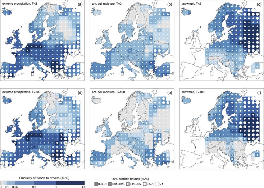
1350 M. Bertola et al.: Regional attribution analysis in Europe
where aT = (yT − y2 )/(y100 − y2 ), with y being the Gumbel In the change model, the flood and covariate data are
reduced variate, which is related to the return period by pooled and used simultaneously to attribute any observed
changes in floods to their drivers. This pooling increases the
1 robustness of the estimates (see, for example, Viglione et al.,
yT = − ln − ln 1 − = − ln (− ln p) . (4)
T 2016) but requires an assumption of homogeneity. Specif-
ically, we assume here that for a given return period and
We adopt the following regional change model accounting
catchment scale, the elasticities of the flood discharges to
for catchment area (S):
their drivers are uniform within the region. We do allow the
drivers to vary between catchments.
ln q2 = ln α20 + γ20 ln S + α21 ln X1 + α22 ln X2
We frame the estimation problem in Bayesian terms
+α23 ln X3 + ε
0
ln x100 = ln αg0 + γg0 ln S + αg1 ln X1 + αg2 ln X2 through a Markov chain Monte Carlo (MCMC) approach,
+αg3 ln X3 , using the R package rStan (Carpenter et al., 2017), which
makes use of a Hamiltonian Monte Carlo algorithm to
ε ∼ N (0, σ ) (5) sample the posterior distribution (Stan Development Team,
2018). For each inference, we generate four chains of 10 000
where X1 , X2 and X3 are three covariates (i.e. time series of
simulations each, with different initial values, and we check
the potential drivers of flood change), and the α and γ terms
for their convergence. We use prior information on the model
represent regional model parameters to be estimated. The ε
parameters to constrain their estimation to hydrologically
term, here assumed normally distributed, is a station-specific
plausible values (see Sect. 2.5).
error term that accounts for additional local variability (i.e.
not explained by catchment area and the covariates) of q2 . 2.2 Spatial correlation of floods
Similar to the index flood method of Dalrymple (1960) and
Hosking and Wallis (1997), we assume here that the growth Spatial correlation of floods is not directly accounted for in
0
curve x100 is the same across all sites within the region (i.e. the proposed regional change model of Sect. 2.1, and it may
it depends on catchment area and the covariates only), while result in underestimated sample uncertainties (see, for ex-
the median flood q2 (the index flood) is allowed to vary be- ample, Stedinger, 1983; Castellarin et al., 2008; Sun et al.,
tween sites, through the error term ε. 2014). Here, we adopt an approach proposed by Ribatet et al.
The elasticity of the generic flood quantile qT with respect (2012) and based on the work of Smith (1990), consisting
to the covariate Xi is defined as in a magnitude adjustment to the likelihood function in a
Bayesian framework, which accounts for the overall depen-
Xi ∂qT 1
ST ,Xi = = α2i + αgi 1 − . (6) dence in space and allows reliable credible intervals to be
qT ∂Xi 0
1 + aT x100 obtained. The adjusted likelihood is defined as
It represents the percentage change in qT , due to a 1 % change L∗ (θ , y) = L(θ , y)k , (10)
in Xi , i.e. how sensitive flood peaks are to changes in the
drivers. However, the elasticity alone does not tell us how where L is the likelihood under the assumption of spatial in-
much the flood quantiles have actually changed (in time) due dependence, θ is the vector of unknown parameters and k
to observed changes of the drivers. Hence, we define the con- is the magnitude adjustment factor to be estimated, such as
tribution of Xi to the changes in qT as 0 < k ≤ 1 (see Appendix A). The magnitude adjustment fac-
tor k represents the overall reduction of hydrological infor-
Xi ∂qT 1 dXi
CT ,Xi = · . (7) mation in the data caused by the presence of spatial correla-
qT ∂Xi Xi dt tion and results in an inflated posterior variance of the param-
It represents the percentage change in qT due to the actual eters. If floods at different sites are spatially independent, k
change in Xi . The total change in qT due to the changes in is 1; on the contrary, if floods are strongly cross-correlated, k
the drivers, assuming that the contributions are additive, is assumes values close to 0. In this latter case, the sample un-
certainty resulting from the adjusted likelihood will be larger,
1 dqT X X Xi ∂qT 1 dXi compared to the model in which spatial cross-correlation is
= CT ,Xi = · . (8)
qT dt qT ∂Xi Xi dt not accounted for. For further details on the adjustment to the
i i
likelihood and its application to hydrological data, see Smith
A measure of relative contribution of Xi to the change in qT (1990), Ribatet et al. (2012) and Sharkey and Winter (2019).
is expressed here by
2.3 Data
abs(CT ,Xi )
RT ,Xi = P , (9) Consistent with Blöschl et al. (2019) and Bertola et al.
i abs(CT ,Xi )
P (2020), we analyse long series of annual maximum dis-
where i RT ,Xi = 1. charges between 1960 and 2010, from 2370 hydrometric sta-
Hydrol. Earth Syst. Sci., 25, 1347–1364, 2021 https://doi.org/10.5194/hess-25-1347-2021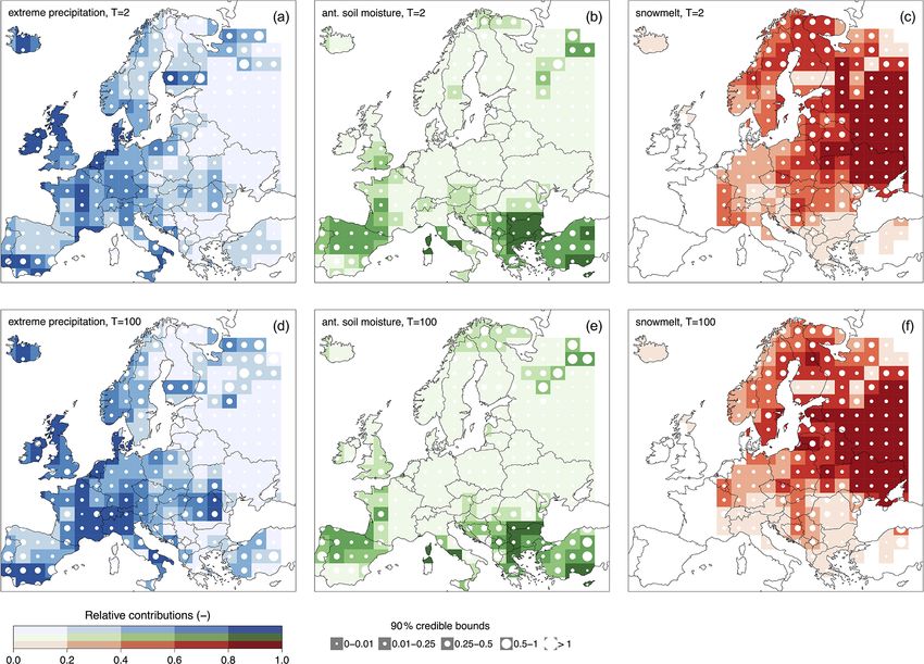
M. Bertola et al.: Regional attribution analysis in Europe                                                                        1351

                                                                       long-term evolution of the drivers, we use average flood sea-
                                                                       sonality and its variability to identify time windows in which
                                                                       drivers are typically relevant for the generation of the an-
                                                                       nual peaks, rather than pairing floods with the correspond-
                                                                       ing event precipitation (which would be instead relevant for
                                                                       event attribution). Unlike in Viglione et al. (2016), scale de-
                                                                       pendence is here accounted for by the data, as we use local
                                                                       (i.e. catchment-averaged) covariates.
                                                                          As in Bertola et al. (2019), this study aims at attribut-
                                                                       ing flood changes to the long-term evolution of the covari-
                                                                       ates rather than their year-to-year variability. For this reason,
                                                                       we smooth the annual series of the drivers with the locally
                                                                       weighted polynomial regression LOESS (Cleveland, 1979)
                                                                       using the R function loess. The subset of data over which the
                                                                       local polynomial regression is performed is 10 years (i.e. 10
                                                                       data-points of the series), and the degree of the local poly-
                                                                       nomials is set equal to 0, which is equivalent to a weighted
                                                                       10-year moving average.
Figure 1. Location of 2370 hydrometric stations in Europe and re-
gions considered in this study. The size of the circles is propor-     2.4.1   Extreme precipitation
tional to the length of flood records. The grid size is 200 km. The
black bordered region shows the size of the spatial moving win-        Daily series of catchment-averaged precipitation between
dows analysed in Sect. 3.2. It consists of nine cells, corresponding   1960 and 2010 are calculated for each hydrometric station
to 600 km × 600 km, whose central cell is shaded black. Three re-      from the daily gridded E-OBS precipitation and the catch-
gions analysed in Sect. 3.3, respectively located in northwestern,     ment boundaries. For each station we identify a window
southern and eastern Europe, are shown with coloured circles, and      around the average date of occurrence of floods D, in which
the shaded regions represent their central cells.                      extreme precipitation is considered to be typically relevant
                                                                       for the generation of the annual peaks. The width of the win-
                                                                       dow w is set between 90 and 360 d, and it is taken propor-
tions in 33 European countries (https://github.com/tuwhydro/           tional to 1 − R, with R being the concentration of the date
europe_floods, last access: 9 April 2020). Stations affected           of occurrence around the average date, through the following
by strong artificial alterations (such as large reservoirs in the      equation:
proximity of the gauges) are not included in this database
(Blöschl et al., 2019). The location of the stations is shown          w = 90 + (1 − R) · 270 [d].                                 (11)
in Fig. 1. Their contributing catchment areas range from 5
to 100 000 km2 , and the median record length is 51 years.             D and R are obtained with circular statistics (see Ap-
The density of stations in the database is highest in central          pendix B). The window of dates is centred around D, in a
Europe and lowest in eastern and southern Europe, where                way that two-thirds of the window occur before the average
time series are generally shorter (Fig. 1). The catchment              date of occurrence of floods (as shown in Fig. 2 for an exam-
boundaries relative to each hydrometric station are derived            ple series in one example year). For each year in the period of
from the CCM River and Catchment Database (Vogt et al.,                interest, we calculate the 7 d maximum precipitation within
2007). Daily gridded precipitation and mean surface temper-            the identified window (which varies between catchments but
ature are obtained from the E-OBS dataset (version 18.0e,              is fixed between years).
resolution 0.1◦ ; Cornes et al., 2018). It covers the area 25–
71.5◦ N × 25◦ W–45◦ E for the period 1950–2018.                        2.4.2   Antecedent soil moisture index

2.4   Drivers of flood change                                          An index of antecedent soil moisture is obtained from daily
                                                                       catchment-averaged precipitation. For each year and each
Because stations with substantial artificial alterations are not       station, we calculate the 30 d precipitation preceding the 7 d
included in the database, in this study we consider three po-          window identified for extreme precipitation above. Longer
tential climatic drivers of flood change: (i) extreme precip-          temporal windows for antecedent precipitation have been as-
itation, (ii) antecedent soil moisture and (iii) snowmelt. For         sessed and did not result in significant differences in terms of
each driver we obtain catchment-averaged time series, as de-           long-term evolution and trend patterns of this driver, even for
scribed in detail in the following paragraphs, which are used          very large catchments. Other precipitation-based soil mois-
as covariates in the regional model of Sect. 2.1. As the in-           ture indices are also available (e.g. the antecedent precipita-
terest of this study resides in attributing flood changes to the       tion index, as defined in Woldemeskel and Sharma, 2016);

https://doi.org/10.5194/hess-25-1347-2021                                           Hydrol. Earth Syst. Sci., 25, 1347–1364, 2021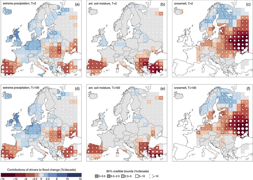
1352 M. Bertola et al.: Regional attribution analysis in Europe
obtained from daily snowmelt, using the same procedure il-
lustrated above for the case of extreme precipitation.
2.5 Prior distributions of model parameters
In the attribution analysis we use informative priors of the
parameters controlling the relationship between flood and co-
variate changes (i.e. the elasticities; see Eq. 6). This is done
because we do not want to use the time patterns of the co-
variates Xi only to discriminate between drivers, which may
lead to spurious correlations, but to “inform” the attribution
analysis based on hydrological knowledge. Therefore, we
set a priori constraints on the model parameters, based on
qualitative reasoning and on prior literature. The changes in
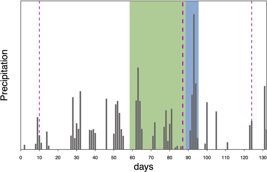
Figure 2. Procedure used to obtain the time series of extreme pre- flood quantiles are expected to be caused by changes of the
cipitation and antecedent soil moisture index. The figure shows the same sign in the drivers, given the covariates considered in
daily series of catchment-averaged precipitation for one example this study (i.e. extreme precipitation, antecedent soil mois-
station in one example year. The thick dashed magenta line repre- ture and snowmelt). For example, increasing floods can be at-
sents the average date of occurrence of annual floods for the ex- tributable to increasing extreme precipitation, while decreas-
ample station, and the two thin dashed lines indicate the window
ing precipitation cannot reasonably cause increasing floods
of dates around the average date of occurrence, where extreme (7 d
maximum) precipitation is selected (blue area). The respective pre-
(which would correspond to a negative elasticity). In other
ceding 30 d precipitation (green area) is representative of the an- words, we expect the elasticity of qT to Xi to be positive. For
tecedent soil moisture. The procedure is repeated for every year in T = 2 and 100 years, this translates respectively into
the period of interest and every hydrometric station.
α 2i > 0 (13a)
1
however they require the definition of additional parameters α2i + αgi 1 − 0 > 0. (13b)
1 + x100
and assumptions (e.g. lag and decay parameters). We use this
index (for brevity, hereinafter referred to as “antecedent soil Eq. 13a represents the lower limit for the elasticity parame-
moisture”) based on precipitation instead of modelled soil ters of q2 . The lower limit for αgi is obtained from Eq. (13b)
moisture, as in Blöschl et al. (2019), in order to more strongly and depends on α2i and on the growth factor:
rely on observational data.
α 2i
αgi > − . (14)
2.4.3 Snowmelt 1 − qq100
2
Similar to precipitation, daily series of catchment-averaged For simplicity, we assume q100 = 2q2 as a reasonable ap-
temperature between 1960 and 2010 are obtained for each proximation valid for Europe (Blöschl et al., 2013; Alfieri
hydrometric station. We calculate daily series of catchment- et al., 2015), and we simplify Eq. (14) to
averaged snowmelt according to a simple degree-day model
(Parajka and Blöschl, 2008) as a function of mean daily air αgi > −2α2i . (15)
temperature TA and precipitation P :
The prior distributions of α2i and on αgi are modelled as nor-
mal distributions N (0, 2) with a truncated lower tail, as sum-
0 for TA < Tm
M= (12a) marised in Table 1. For the remaining parameters, we set an
min (DDF · (TA − Tm ); Ps ) for TA ≥ Tm
improper uniform prior distribution.
P for TA < TS
PS = P · TTRR−T
−TS
A
for TS ≤ TA ≤ TR , (12b) 2.6 Regional analyses
0 for TA > TR
Following the spatial moving window approach of Bertola
where M and Ps are the daily snowmelt depth and snow wa- et al. (2020), we identify several regions of size
ter equivalent storage, DDF is the degree-day factor and Tm , 600 km × 600 km across Europe, which overlap by 200 km
TS and TR are the temperature thresholds that control the oc- in both directions. We fit the regional flood change model of
currence of melt, snow and rainfall, respectively. Here we as- Sect. 2.1 to pooled flood and covariate data of sites within
sume Tm = TS = 0◦ C, TR = 2.5◦ C and DDF = 2.5 mm per each region. The resulting 200 km × 200 km grid cells are
day per ◦ C (Parajka and Blöschl, 2008; He et al., 2014). For shown in Fig. 1, and each of the considered regions is com-
each station, the time series of 7 d maximum snowmelt is posed of nine adjacent cells, (e.g. the black bordered region
Hydrol. Earth Syst. Sci., 25, 1347–1364, 2021 https://doi.org/10.5194/hess-25-1347-2021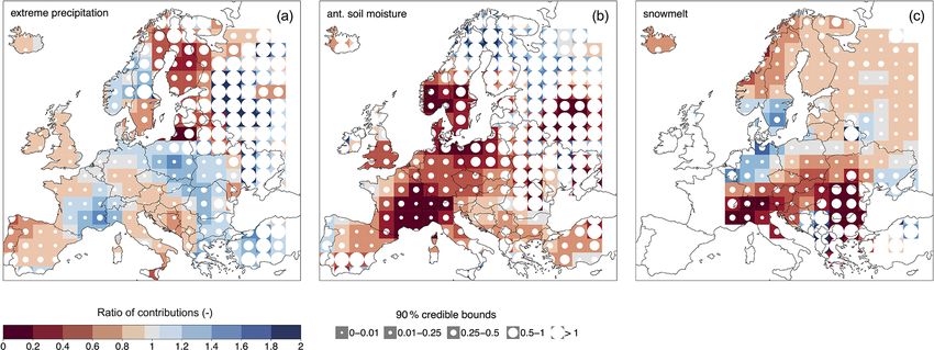
M. Bertola et al.: Regional attribution analysis in Europe 1353
Table 1. Priors of model elasticity parameters controlling the relationship between flood and covariate changes.
Parameter Meaning Lower limit Distribution type
α21 Elasticity of q2 to X1 0 Truncated normal
α22 Elasticity of q2 to X2 0 Truncated normal
α23 Elasticity of q2 to X3 0 Truncated normal
αg1 0
Elasticity of x100 to X1 −2α21 Truncated normal
αg2 0
Elasticity of x100 to X2 −2α22 Truncated normal
αg3 0
Elasticity of x100 to X3 −2α23 Truncated normal
in Fig. 1). All station-years contribute to the likelihood, and ticularly in the Alpine region and on the western Atlantic
the likelihood is corrected using the magnitude adjustment coast. Positive changes of extreme precipitation are observed
to account for spatial cross-correlation between sites. The ra- in the Alpine region, northwestern and central Europe, Scan-
tionale behind the homogeneity assumption is that the spatial dinavia and Poland; negative changes are observed in south-
windows, given their size, are characterised by rather homo- ern countries and in few spots in central Europe (Fig. 3d).
geneous climatic conditions relative to the overall variability Similar spatial patterns appear for antecedent soil moisture
within Europe. (Fig. 3b and e), but the negative changes tend to be more
In each region, we estimate the elasticity of q2 and q100 widespread and with stronger (negative) magnitude. Mean
to the drivers Xi and the contribution of each driver to flood snowmelt is largest in northeastern Europe and in the Alpine
changes, obtained by multiplying the elasticity by the aver- region (Fig. 3c). Its changes are mostly negative across all
age driver trend in the region (Eq. 7). In regions where the Europe, with the exception of the very north and a few iso-
average 7 d maximum snowmelt is less than 2 mm per day, lated spots (Fig. 3f).
only extreme precipitation and antecedent soil moisture are
considered as potential drivers (i.e. Eq. 5 is modified by re- 3.2 Contributions of the drivers to flood change across
moving the contribution of X3 ). The resulting elasticity and Europe
contribution are plotted in the central 200 km × 200 km cell
of the region (e.g. the shaded cell in the black bordered region The obtained time series of catchment-averaged extreme pre-
in Fig. 1). The results are shown for a hypothetical catch- cipitation, antecedent soil moisture and snowmelt are used as
ment area S = 1000 km2 , corresponding to a medium-sized covariates in the regional driver-informed model of Sect. 2.1.
catchment. This is because it is of interest to show average Figure 4 shows maps of the elasticity of the 2-year flood q2
driver contributions to changes in flood quantiles within each and the 100-year flood q100 to each of the three drivers, as
region, rather than model results corresponding to an exist- defined in Eq. (6), resulting from fitting the regional model
ing single catchment in the region. The attribution analysis to the pooled flood and covariate data in moving windows
is thereby performed at the regional scale, where average re- across Europe. The elasticities are measured here in percent
gional contributions of the decadal changes in the drivers to per percent (%/%) and represent the percentage change in
average regional trends in flood quantiles are estimated. The qT , due to a 1 % change in Xi , i.e. how sensitive flood peaks
results of this analysis are shown in Sect. 3.2. In Sect. 3.3, are to changes in the drivers. The value of the posterior me-
the elasticities of flood quantiles to the drivers and their con- dian of the elasticities is shown together with the 90 % cred-
tributions to flood change are further analysed as a function ible bounds, which represent a measure of the uncertainty
of the return period, for three regions located respectively in associated with the estimate and take into account the differ-
northwestern, southern and eastern Europe (see Fig. 1). ent density of stations across Europe (i.e. larger uncertainties
are typically observed in data-scarce regions).
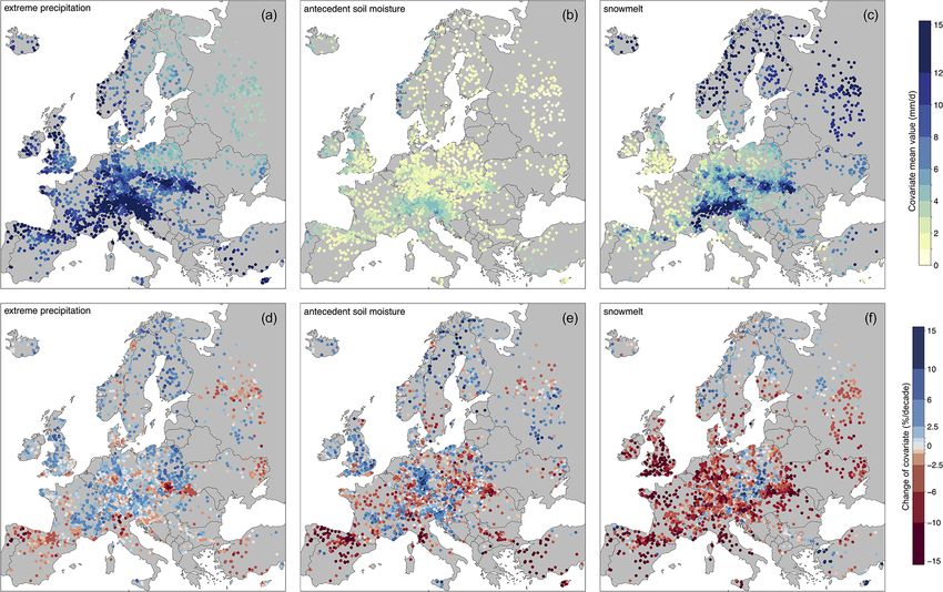
The elasticity of q2 to extreme precipitation (Fig. 4a) is
3 Results large (0.6 to 1.5) in western, central and southern Europe
(indicating that the 2-year flood increases by 0.6 % to 1.5 %
3.1 Drivers of flood change if extreme precipitation increases by 1 %), and lower values
(0 to 0.25) are observed in northeastern Europe (i.e. the 2-
Time series of catchment-averaged (i) extreme precipitation, year flood increases by 0 % to 0.25 % following a 1 % in-
(ii) antecedent soil moisture and (iii) snowmelt are obtained crease in extreme precipitation). Similar values of elasticity
for each hydrometric station for the period 1960–2010, as to extreme precipitation are observed for the 100-year flood
described in Sect. 2.4. Figure 3 shows maps of the mean across Europe (Fig. 4b), with small differences in northeast-
value and the change of these drivers for each station in the ern Europe. This means that the elasticity of flood quantiles
period of interest. Extreme precipitation (Fig. 3a) exhibits to extreme precipitation does not vary much with return pe-
its largest mean values in central and western Europe, par- riod. In contrast, the elasticity of flood quantiles to soil mois-
https://doi.org/10.5194/hess-25-1347-2021 Hydrol. Earth Syst. Sci., 25, 1347–1364, 2021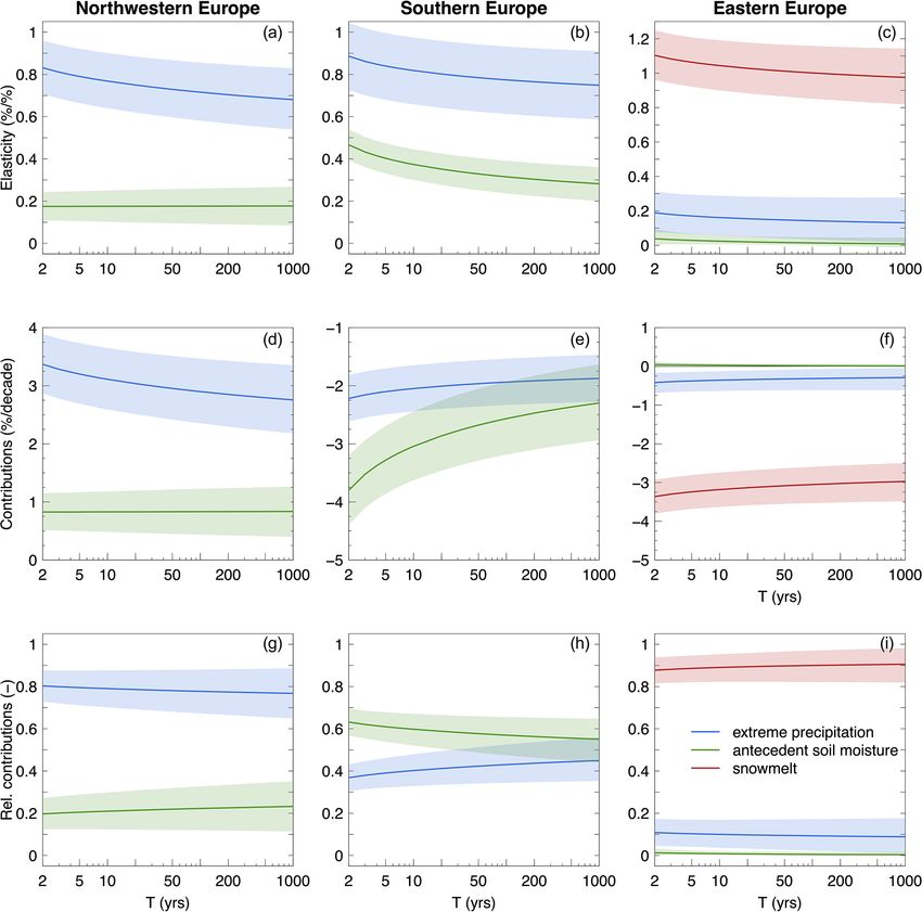
1354                                                                   M. Bertola et al.: Regional attribution analysis in Europe

Figure 3. Mean value and change of catchment-averaged extreme precipitation (a, d), antecedent soil moisture (b, e) and snowmelt (c, f) for
each station over the period 1960–2010.

ture decreases with return period (i.e. q2 increases more than          tive flood changes in southern Europe, and the magnitude of
q100 if soil moisture increases by 1 %), and it is largest in           this contribution is smaller in absolute values for large floods
southern Europe (0.25 to 0.6; Fig. 4b and 4e). Overall, the             than for the median floods (Fig. 5b and e). Snowmelt (Fig. 5c
elasticities of q2 and q100 to soil moisture are smaller than           and f) contributes to marked negative changes in q2 and q100
those to extreme precipitation. The elasticity of floods to             in eastern Europe and to positive flood changes in northern
snowmelt is largest in northeastern Europe (Fig. 4c and d),             Europe. We overall observe smaller contributions in absolute
where values above 1 are observed (i.e. a change of 1 % in              values to changes in q100 than q2 . In data-scarce regions the
snowmelt translates into a change in flood quantiles larger             credible bounds tend to be larger; i.e. the attribution results
than 1 %). In northeastern Europe the elasticities of q2 and            have larger uncertainties. Overall the uncertainties associated
q100 to snowmelt are similar, while in central Europe and the           with the contribution of the drivers to changes in q100 do not
Balkans they decrease with the return period.                           seem to increase much compared to q2 .
   Figure 5 shows maps of the contributions of each of the                 In order to further investigate the differences in terms of
three drivers to changes in q2 and q100 , as defined in Eq. (7).        (absolute) contributions of the drivers to changes in large (i.e.
They are obtained by multiplying the elasticities of flood              q100 ) versus small floods (i.e. q2 ), we compute for each driver
quantiles to the drivers by the average changes (in percent per         the ratio between these two quantities (Fig. 6). In the case of
decade) in the drivers in each region over the period 1960–             extreme precipitation (Fig. 6a), the ratio between its contri-
2010 (Eq. 7). They represent the change in flood quantiles,             butions to changes in q100 and q2 is between 0 and 1 in the
in percent per decade, caused by the change in a specific               Atlantic region, Spain, Italy, the Balkans, southern Germany,
driver. Extreme precipitation (Fig. 5a and d) contributes to            Austria and Finland; i.e. in these regions the contribution of
positive flood changes in northwestern and central Europe               extreme precipitation to changes in q100 is smaller, in abso-
and to negative flood changes in southern and eastern Eu-               lute value, compared to changes in q2 . In southern France,
rope. The absolute value of the contributions of extreme pre-           eastern Europe and Turkey, the opposite is observed (i.e. the
cipitation appears to slightly decrease when moving from q2             ratio is larger than 1). Antecedent soil moisture and snowmelt
to q100 . Antecedent soil moisture contributes mostly to nega-          generally contribute less to changes in q100 compared to q2

Hydrol. Earth Syst. Sci., 25, 1347–1364, 2021                                             https://doi.org/10.5194/hess-25-1347-2021
M. Bertola et al.: Regional attribution analysis in Europe                                                                                 1355

Figure 4. Elasticity of the 2-year flood q2 (upper panels) and the 100-year flood q100 (lower panels) to extreme precipitation (a, d), antecedent
soil moisture (b, e) and snowmelt (c, f). The median value of the posterior distribution of the elasticity is shown in each region with colours,
and the size of the white circles is proportional to the respective 90 % credible bounds. The maps are shown for a hypothetical catchment
area of 1000 km2

(i.e. the ratio is < 1; Fig. 6b and c). Large uncertainties in             moisture gives the largest relative contribution to changes in
the ratio of elasticities are observed in northeastern Europe,             q2 (Fig. 7b), and its relative importance tends to decrease
in the case of extreme precipitation and antecedent soil mois-             for more extreme floods (Fig. 7e). The relative contribution
ture (Fig. 6a and b), and in southern Europe, in the case of               of snowmelt to flood changes clearly prevails over the other
snowmelt (Fig. 6c). They result from values of the contribu-               drivers in eastern Europe, with slightly decreasing strength
tion of the drivers to q2 that are close to zero (see Fig. 5), indi-       for the higher return period.
cating that, in these regions, flood changes are not explained
by changes in extreme precipitation or antecedent soil mois-               3.3   Contributions to flood change of the drivers in
ture.                                                                            northwestern, southern and eastern Europe
   Finally, for each region we obtain the relative contribution
of the three drivers to changes in q2 and q100 , as defined in             In this section we select three example regions among those
Eq. (9) (Fig. 7). They represent the fraction of the regional              analysed in Sect. 3.2, located respectively in northwestern,
trend in flood quantiles qT that is explained by changes in                southern and eastern Europe (see Fig. 1). For these three re-
one driver. The relative contribution of extreme precipitation             gions we further show in Fig. 8 the elasticities of floods to the
is the largest of all the drivers in most of western and cen-              drivers (first row), the contributions (second row) and relative
tral Europe for both q2 and q100 (Fig. 7a and d). The rela-                contributions (third row) of the drivers to flood change, as a
tive contribution is slightly smaller for large floods than for            function of the return period. In the regions located in north-
the median flood in northwestern Europe, while the opposite                western and southern Europe, snowmelt is excluded from the
is the case in the south. In southern Europe antecedent soil               potential drivers as it does not represent a relevant process for

https://doi.org/10.5194/hess-25-1347-2021                                                 Hydrol. Earth Syst. Sci., 25, 1347–1364, 2021
1356                                                                       M. Bertola et al.: Regional attribution analysis in Europe

Figure 5. Same as Fig. 4 but for contributions of extreme precipitation (a, d), antecedent soil moisture (b, e) and snowmelt (c, f) to changes
in q2 and q100 .

Figure 6. Same as Fig. 4 but for the ratios of the contributions of extreme precipitation (a), antecedent soil moisture (b) and snowmelt (c) to
changes in q100 relative to q2 . Values below 1 (red colour) indicate that the contribution of the driver to q100 is smaller than the contribution
to q2 ; values above 1 (blue colour) indicate that the contribution of the driver to q100 is larger than the contribution to q2 .

Hydrol. Earth Syst. Sci., 25, 1347–1364, 2021                                                 https://doi.org/10.5194/hess-25-1347-2021
M. Bertola et al.: Regional attribution analysis in Europe                                                                               1357

Figure 7. Same as Fig. 4 but for relative contributions of extreme precipitation (a, d), antecedent soil moisture (b, e) and snowmelt (c, f) to
changes in q2 and q100 .

most of the catchments in these regions (see Fig. 3c). Addi-              extreme precipitation increases and becomes comparable to
tionally, in Fig. 9, flood and driver time series are shown for           that of antecedent soil moisture (Fig. 8h). The contribution
the stations in each of the three regions, as well as their aver-         of snowmelt to flood changes clearly dominates in the region
age changes in time within the regions.                                   located in eastern Europe at all return periods (Fig. 8c, f and
   In the region in northwestern Europe, both extreme pre-                i).
cipitation and antecedent soil moisture contribute to posi-                   In this latter case, we observe that the posterior distribution
tive flood changes, with extreme precipitation representing               of the elasticity of qT to antecedent soil moisture (represent-
the most important driver. Its contribution to flood trends de-           ing the change in flood quantiles due to a 1 % change in the
creases with increasing return period, while the contribution             driver) is concentrated and flattened around zero. This results
stays almost constant in the case of antecedent soil moisture             from the adopted informative priors of the elasticity parame-
(Fig. 8d and g). In the region in southern Europe extreme pre-            ters, which set their lower bound to zero, in order to exclude
cipitation and antecedent soil moisture represent both impor-             hydrologically implausible values (i.e. a negative elasticity
tant drivers. The elasticity of floods to extreme precipitation           would imply that decreasing floods are attributed to increas-
is larger than that to antecedent soil moisture (Fig. 8b). How-           ing antecedent soil moisture, or vice versa; see Sect. 2.5).
ever, antecedent soil moisture contributes to a larger extent to          In fact, antecedent soil moisture slightly increases over time
negative flood changes for small return periods (i.e. T = 2–              in this region (Fig. 9f), while flood magnitude decreases for
10 years) due to larger (negative) changes in antecedent soil             both T = 2 and 100 years (Fig. 9i). As a consequence, the
moisture (Fig. 9b and e). Its contribution decreases in abso-             elasticity would tend to be negative (in case non-informative
lute values with increasing return period (Fig. 8e). For more             priors on the elasticity parameters are adopted), but it is con-
extreme events (T > 10 years) the relative contribution of                strained by the lower bound of the priors.

https://doi.org/10.5194/hess-25-1347-2021                                               Hydrol. Earth Syst. Sci., 25, 1347–1364, 2021
1358                                                                        M. Bertola et al.: Regional attribution analysis in Europe

Figure 8. Contributions of drivers to flood changes as a function of the return period in three regions (columns), respectively located in
northwestern, southern and eastern Europe. Elasticity of floods to the drivers (a, b, c), contribution (d, e, f) and relative contribution (g, h, i)
of the drivers to flood change are shown in the rows. The thick lines and the shaded areas represent the median and the 90 % credible intervals
of their posterior distributions, respectively. The results are shown for a hypothetical catchment area of 1000 km2 .

4   Discussion and conclusions                                              4.1    Is it possible to identify the relative contributions of
                                                                                   different drivers to q100 changes as compared to q2
In this study, we attribute the changes in flood discharges                        changes?
that have occurred in Europe during the period 1960–2010
(Blöschl et al., 2019; Bertola et al., 2020) to potential drivers
                                                                            Our results suggest that in northwestern and eastern Eu-
as a function of the return period, while previous detection
                                                                            rope, changes in small and large floods are driven mainly
and attribution studies have generally focused on the mean
                                                                            by one single driver, which dominates at all return periods.
flood behaviour. In particular, we compare the relative contri-
                                                                            In northwestern Europe, extreme precipitation contributes to
bution of extreme precipitation, antecedent soil moisture and
                                                                            changes in both q2 and q100 for the most part, and the con-
snowmelt to changes in the median and the 100-year flood.
                                                                            tribution of antecedent soil moisture is of secondary impor-
The attribution study is framed in terms of a non-stationary
                                                                            tance. Similarly, in eastern Europe, snowmelt clearly drives
flood frequency analysis, and the parameters of the distribu-
                                                                            flood changes at all return periods. In southern Europe both
tion are estimated in a regional context with Bayesian infer-
                                                                            antecedent soil moisture and extreme precipitation signifi-
ence. The study focuses on the average regional behaviour
                                                                            cantly contribute to flood changes, and their relative impor-
and flood attribution at the large scale. The results of the
                                                                            tance depends on the return period. Antecedent soil mois-
study should therefore be interpreted at the continental scale
                                                                            ture contributes the most to changes in small floods (i.e.
as average contributions of the drivers to flood changes in the
                                                                            T = 2–10 years), while the two drivers contribute with com-
regions, rather than at the catchment scale.
                                                                            parable magnitude to changes in more extreme events (T >
                                                                            10 years). Given the relative driver contributions and their
                                                                            credible bounds obtained in the analysis, the findings suggest

Hydrol. Earth Syst. Sci., 25, 1347–1364, 2021                                                   https://doi.org/10.5194/hess-25-1347-2021
M. Bertola et al.: Regional attribution analysis in Europe 1359
Figure 9. Driver and flood time series in three regions, respectively located in northwestern, southern and eastern Europe. Thin lines represent
flood and covariate time series for each station in the three regions. Thick lines in panels (a) to (f) represent the median. Thick lines in
panels (g) to (i) represent the posterior median of the flood quantiles, and the shaded regions are the respective 90 % credible bounds.
Numbers in panels (a) to (f) refer to the average changes in the drivers. Numbers in panels (g) to (i) refer to the sum of the contributions
of the three drivers to changes in q2 (black) and q100 (magenta), i.e. to the average changes in q2 and q100 resulting from this model for
S = 1000 km2 .
that it is indeed possible to identify the relative contributions that the changes in flood quantiles potentially caused by the
to changes in q2 and q100 with the presented approach. three considered drivers are overall compatible, in terms of
patterns and magnitude, with the flood changes observed in
4.2 What is the nature (sign and magnitude) of these previous studies (Blöschl et al., 2019; Bertola et al., 2020).
contributions? Some discrepancies are nevertheless observed, for instance,
in Scandinavia, where the contributions of the drivers are
Extreme precipitation contributes to positive flood changes all positive or close to zero, while mostly moderate negative
in northwestern Europe (about 3.3 % to 2.8 % per decade in flood trends were observed in previous studies. This discrep-
Fig. 8), and its effect decreases slightly with return period ancy points to other drivers not accounted for in the presented
in the region analysed in Sect. 3.3. In contrast, in the re- model, such as river regulation effects (Arheimer and Lind-
gion selected in southern Europe, extreme precipitation con- ström, 2019), or non-linear relationships between the drivers
tributes to 37 % to 45 % of the negative flood changes (cor- not captured by the model.
responding to −2.2 % to −1.8 % per decade), depending on
the return period. The contribution of antecedent soil mois- 4.3 Discussion of model assumptions
ture is negative in southern Europe and decreases in abso-
lute value (from −3.8 % to −2.3 % per decade) with the re- One of the main assumptions in our analysis is that the
turn period in the analysed region. Finally, in eastern Europe three drivers (i.e. extreme precipitation, soil moisture and
snowmelt strongly contributes to negative flood changes in a snowmelt) are the only candidates for explaining river flood
similar way at all return periods (about −3 % per decade for changes. This selection is motivated by recent studies point-
the region in Sect. 3.3). This study more generally suggests ing out potential correlations between timing and magnitude
https://doi.org/10.5194/hess-25-1347-2021 Hydrol. Earth Syst. Sci., 25, 1347–1364, 20211360 M. Bertola et al.: Regional attribution analysis in Europe
of floods and the considered drivers across Europe (Blöschl already stated, the presented results should be interpreted at
et al., 2017, 2019; Berghuijs et al., 2019; Kemter et al., 2020). the European scale. Average driver contributions to changes
The effects of other drivers not accounted for in this study, in flood quantiles over the 5 analysed decades are presented,
such as land-cover change or river regulation, are probably and this study does not aim at estimating driver contributions
not very large at the scale of Europe as we are focusing locally, in ungauged basins.
on catchments with minimum alteration. However, in con- Spatial cross-correlation of floods at different sites is taken
texts where anthropogenic alterations are important, it will into account through an approach based on a magnitude ad-
be useful to extend the analysis for such effects. This attri- justment to the likelihood. This results in larger uncertain-
bution analysis may be repeated with catchment (e.g. land- ties of the posterior distribution of the estimated parameters,
use or land-cover changes) and river drivers (e.g. construc- compared to the case in which floods are considered spatially
tion of reservoirs in the catchment) in addition to atmo- independent. Overall the obtained uncertainties associated
spheric covariates, if detailed information about changes in with the contribution of the drivers to changes in q100 do not
land use/land cover and river structures were available for seem to increase much compared to q2 , while a relevant in-
European catchments and flood data of affected stations were crease would be reasonably expected. These results are valid
collected. under the assumption of the adopted model (i.e. Gumbel dis-
In this study, we directly model the changes in flood quan- tribution), which may be too stringent. The model assump-
tiles because, in a Bayesian framework, it is typically easier tions could be relaxed (e.g. adopting a generalised extreme
for experts to formulate prior beliefs in terms of flood quan- value distribution) in order to allow for larger model flexibil-
tiles associated with large return periods, which they are fa- ity.
miliar with, rather than in terms of distribution parameters
(see, for example, the causal information expansion based on
expert judgement in Viglione et al., 2013). Prior information 5 Conclusions
on the elasticities is used in order to “inform” the attribution
This study represents a continental-scale attribution analy-
analysis, based on hydrological reasoning and the literature.
sis and complements recent research on past changes in Eu-
Specifically, the prior distribution of the elasticities of q2 and
ropean floods by formally attributing the detected trends to
q100 to the drivers is assumed positive. This is because any
potential drivers (i.e. extreme precipitation, antecedent soil
changes in the considered covariates are expected to translate
moisture and snowmelt) as a function of return period. We
into flood changes with the same sign. In practice, the prior
propose a new data-based attribution approach to estimate
distribution of the elasticity of q100 is reflected in a lower
driver contributions to changes in flood quantiles at the re-
bounded prior distribution of the elasticity of the growth fac-
0 , which depends on the ratio between q gional scale. This approach may be generalised and applied
tor x100 100 and q2
in other regions, where the explanation of past flood changes
(Sect. 2.5). For simplicity, we assume this ratio to be equal
is of interest. The results show that in northwestern and east-
to 2. This assumption is reasonably valid for humid catch-
ern Europe, changes in both the 2-year and the 100-year flood
ments (see, for example, Blöschl et al., 2013) and is in over-
are driven by a single driver only (i.e. respectively extreme
all agreement with flood maps of the mean annual flood and
precipitation and snowmelt), while in southern Europe, two
q100 in Europe presented by Alfieri et al. (2015). However,
drivers contribute to flood changes (i.e. soil moisture and
in arid regions, larger values of this ratio (e.g. 4; see Blöschl
extreme precipitation), with different relative contributions
et al., 2013) would be more appropriate (corresponding to
depending on the return period. The results of this study
stricter priors on the elasticity of the growth factor) because
contribute to improved understanding of past flood changes
the flood frequency curves tend to be steeper.
across Europe over the past 5 decades.
The change model of Sect. 2.1 is fitted to the pooled
flood and covariate data of several regions across Europe,
where elasticities of flood quantiles to their drivers are as-
sumed homogeneous. The rationale behind the homogene-
ity assumption is that the spatial windows, given their size,
are characterised by rather homogeneous climatic conditions
and presumably processes driving flood changes, relative to
the overall variability within Europe. The attribution analysis
is thereby performed at the regional scale, where average re-
gional contributions of the decadal changes in the drivers to
average regional trends in flood quantiles are estimated. Even
though we have not assessed the statistical homogeneity of
the regions in terms of the flood change model used here, we
expect the effect of heterogeneity on the average regional be-
haviour to be less relevant than for the local behaviour. As
Hydrol. Earth Syst. Sci., 25, 1347–1364, 2021 https://doi.org/10.5194/hess-25-1347-2021M. Bertola et al.: Regional attribution analysis in Europe 1361
Appendix A: Adjustment to the likelihood
Under the assumption of spatial independence of the
data, the asymptotic distribution of the maximum likeli-
estimator θ̂ of
hood the independence likelihood is θ̂ ∼
0 −1 −1
N θ ,n H V H −1 , where θ 0 is the true value of θ ,
and H −1 V H−1 is the modified covariance
matrix, where
H = −E∇ 2 l θ 0 , y and V = Cov∇l θ 0 , y . If the assump-
tion of spatial independence is correct, we have H = V . In
Sect. 2.2 we described an approach, proposed by Ribatet
et al. (2012), that enables spatial cross-correlation to be ac-
counted for in spatial datasets and consists in an overall ad-
justment to the likelihood. In this analysis we adopted a mag-
nitude adjustment, through a factor k (Eq. 10). Ribatet et al.
(2012) proposed to estimate k by setting
p
k = Pp , (A1)
i=1 λi
where p is the number of parameters in the independence
likelihood, and λi are the eigenvalues of the matrix H −1 V .
The matrix H isapproximated by the observed information
matrix ∇ 2 l θ̂, y , and V is estimated by decomposing the
likelihood into independent yearly contributions.
Appendix B: Seasonality of floods
As in Blöschl et al. (2017), the average date of occurrence of
floods D and the concentration R of the date of occurrence
around the average date are obtained with circular statistics,
by conversion of the date of occurrence of a flood in the year
i into an angular value Di :
tan−1 y · m x > 0, y ≥ 0
x 2π
D = tan−1 yx + π · 2π
m
x≤0 (B1a)
−1 y
m
tan x + 2π · 2π x > 0, y ≤ 0
q
R = x2 + y2, (B1b)
with
n
1X
x= cos θi (B2a)
n i=1
n
1X
y= sin θi (B2b)
n i=1
2π
θi = Di · , (B2c)
mi
where n is the number of peaks registered at that station, mi is
the number of days in the year i and m is the average number
of days per year. When floods occur equally throughout the
year, R = 0, while R = 1 when floods always occur on the
same date.
https://doi.org/10.5194/hess-25-1347-2021 Hydrol. Earth Syst. Sci., 25, 1347–1364, 2021You can also read