Evaluating the Approaches of Small Area Estimation Using Poverty Mapping Data
←
→
Page content transcription
If your browser does not render page correctly, please read the page content below
Journal of Statistical and Econometric Methods, Vol.10, No.2, 2021, 1-21
ISSN: 2241-0384 (print), 2241-0376 (online)
https://doi.org/10.47260/jsem/1021
Scientific Press International Limited

           Evaluating the Approaches of Small Area
           Estimation Using Poverty Mapping Data
         Md. Mizanur Rahman1, Deluar J. Moloy2 and Md. Sifat Ar Salan3

                                           Abstract

Nowadays, estimation demand in statistics is increased worldwide to seek out an
estimate, or approximation, which may be a value which will be used for various
purpose, albeit the input data could also be incomplete, uncertain, or unstable. The
development of different estimation methods is trying to provide most accurate
estimate and estimation theory deals with finding estimates with good properties.
The demand of small area estimation (SAE) method has been increasing rapidly
around the world because of its reliability compared to the traditional direct
estimation methods, especially in the case of small sample size. This paper mainly
focuses on the comparison of several indirect small area estimation methods (post-
stratified synthetic, SSD and EB estimates) with traditional direct estimator based
on a renowned data set. Direct estimator is approximately unbiased but SSD and
Post-stratified synthetic estimator is extreme biased. To cope up the problem, we
conduct another model-based estimation procedure namely Empirical Bayes (EB)
estimator, which is unbiased and compare them using their coefficient of variation
(CV). To check the model assumption, we used Q-Q plot as well as a Histogram to
confirm the normality, bivariate correlation, Akaike information criterion (AIC).

JEL classification numbers: C13, C51, C51.
Keywords: Small Area Estimation, Direct Estimation, Indirect Estimation,
Empirical Bayes Estimator, Poverty Mapping.

1
    Department of Statistics, Mawlana Bhashani Science and Technology University, Bangladesh.
2
    Department of Statistics, Mawlana Bhashani Science and Technology University, Bangladesh.
3
    Department of Statistics, Mawlana Bhashani Science and Technology University, Bangladesh.

Article Info: Received: February 1, 2021. Revised: May 5, 2021.
Published online: May 10, 2021.
2 Rahman et al. 1. Introduction Sample survey is a method of data collection with several advantages, such as saving time, money, and energy. Sample survey usually produced reliable estimated value usually direct estimate for mean or total of variable of interest for large areas or domain. Nevertheless, if there is a small area, i.e., if the sample is not large enough for some context, the result can be unacceptably large standard errors if it is based only on direct survey estimators and data from the sample field only. So to develop more reliable estimated value, it is important to use small area statistics. In recent years, interest from both the public and private sectors for accurate estimates for a specific region or area has grown. The word "small area" generally refers to a population for which accurate statistics of interest cannot be produced, due to certain constraints of the available data. Small area comprises a geographic area such as states, counties, districts, or sub-districts and population community such as age, ethnicity, or gender (S Hariyanto, 2018). Some of the other words that are used as a synonym for a small area include "small domain," "minor domain," "local area," "small sub-domain" (Rao 2003). Finally, it can be define that small area estimation (SAE) is a statistical technique to estimate the accurate approximation or estimate in the small geographical area where the sample size is very small or even equal to zero. In situations where direct estimates cannot be disseminated due to unsatisfactory accuracy, an ad hoc collection of methods, called methods for small area estimating (SAE), is necessary to overcome the problem. These methods are usually referred to as indirect estimators since they handle poor information from sample information belonging to other domains for each domain borrowing strength, resulting in an increase in the effective sample size for each small area. The growing requirement for more timely and accurate information, along with the high cost of interviews, frequently leads to comprehensive use of survey data. In fact, survey data is used many times to generate estimates in smaller domains or areas than those for which the survey was originally planned. A direct estimator, relying solely on the survey data coming from that area, maybe very inefficient for a region with a low sample size. This sample size limitation prevents statistical figures from being produced at the demanded level and therefore limits the availability of statistical information to the public or the specific user. By comparison, through increasing the effective sample size, an indirect estimator for a region often uses external data from other areas to improve performance. Among indirect estimators, we consider the ones based on explicit models of regression, called model based estimators. These estimators are focused on the presumption of a constant link between the target variable and certain explanatory variables through areas. The common parameters of the model are estimated using the whole set of sample data, which often leads to small area estimators with significantly better efficiency than direct estimators as long because the assumptions of the model hold. Thus, these strategies include statistical figures
Evaluating the Approaches of Small Area Estimation Using Poverty Mapping Data      3

at a much-disaggregated level without raising the area-specific sample sizes and
hence without raising the survey cost.
The key purposes of this research are to evaluate and comparison of various small
area estimation approaches using poverty mapping data. In this paper, we use
several table and figure to compare these methods.
Research methods define as the technique of strategy those are used for conduction
of a research. All methods which are used by the researcher during the course of
studying his research problem are termed as research method. In this paper, we will
use the following methodologies:
1) Horvitz-Thompson (H-T) estimation use for direct estimation.
2) Post-stratified synthetic indirect estimator use based on statistical approach on
    implicit models.
3) Empirical Bayes (EB) method indirect estimator use based on statistical
    approach on explicit models.
4) Mean square error (MSE).
For checking the model assumption, we use the following method:
1. Q-Q plot, as well as Histogram, used to confirm the normality assumption.
2. Bivariate correlation.
3. Akaike information criterion (AIC).

2. Previous work on poverty mapping indicator
Poverty maps are an important source of information on the regional distribution of
poverty and are currently used to support regional policy making and to allocate
funds to local jurisdictions. Good examples are the poverty and inequality maps
produced by the World Bank for many countries all over the world. Some previous
work on poverty mapping using small area estimation are given below:
One paper (Novi Hidayat Pusponegoro, 2019) seeks to compare the SAE, Spatial
SAE and Geo-additive model for calculating a sub-district average per capita
income using data from the 2017 Bangka Belitung Province Poverty Survey. The
paper's findings are the Geo-additive is the best fit model based on AIC, so the most
important part of modeling is the form of relationship between response and
covariate.
The research (Mai M. Kamal El Saied, 2019) is to study the SAE procedures for
estimating the Egyptian provinces ' mean income and poverty indicators. They
demonstrated the direct estimators for mean income and poverty indicators for all
provinces. This research also applies the empirical best / Bayes (EB) and pseudo-
empirical best / Bayes (PEB) approaches focused on unit level -nested error- models
for estimating mean income and (FGT) deprivation indices for Egyptian border
provinces with (2012-2013) data from the IECS. For comparative purposes, the
(MSEs) and coefficient of variance (C. Vs) are determined.
Results (Hukum Chandra, 2018) in district-specific values suggest that the
approximate assessments of the proportion of poor households in each district are
unreliable, with CVs ranging from 13.33% to 64%, with an average of 24.69%. The
4 Rahman et al. CVs of the EBP estimates range from 12.96% to 37.27%, with 21.19% on average. It also noted that the direct estimates CVs are greater than 20 percent (30 percent) in 22 (9) of the 38 districts. However, out of the 38 districts, the model-based estimates are greater than 20 per cent (30 per cent) in 20 (3). The paper (Mai M. Kamal El Saied, 2019) approximate mean income indicates that for all provinces, PEB and EB divided by regional sample sizes have no noticeable differences except for the third of sample size (Red Sea), the PEB therein is greater than the EB. The C.Vs for PEB are smaller than the C.Vs for EB in all selected provinces except the sec for PEB on it is greater than the C.V for EB. The estimated C.Vs are still under 15% for both methods in all selected provinces. EB estimates for poverty incidence and poverty gap are smaller than PEB for all provinces. Additionally, that the differences are large in three provinces (Matruh, North Sinai and South Sinai), and are small in two of them (Red Sea and New Valley). Estimated poverty rate and poverty gap figures for C.Vs for EB, as predicted. Paper (Molina, 2009) showed that the estimated CVs of direct estimators of poverty incidences exceeded the level of 10% for 78 (out of the 104) domains, while those of the EB estimators exceeded this level for only 28 domains. If we increase the level to 20%, then the direct estimators have a greater CV for 17 domains but the CV of EB estimators exceeded 20% only for the first domain. In March 2017, the Province of Yogyakarta Special Region (DIY Province) had a poverty line above the national average of IDR 374,009, a proportion of poor people (13.03%) and Gini coefficient (0.432) (IDR 374,478; 10.64%; 0.393). The outcome of the 2017 happiness index indicates that DIY Province's position (72.93%) is higher than the national happiness index average (70.69%). For 2017, the dispersal between the index of satisfaction and the proportion of poor people for Indonesia indicates that DIY Province is on the first quadrant. It reflects the high level of happiness as well as the high percentage of the poor. To assess the spatial characteristics of deprivation and happiness profiles in DIY Province, a small area estimate approach developed by Elbers et al. (known as the ELL method) is used. This study utilized data from the village census (Podes) 2018; Susenas March 2017 and SPTK 2017 as data from the survey. There are twenty-three variables for households and another five variables that are significant to urban and rural provincial models of poverty and happiness. Rural regency areas are dominated by a high profile of poverty (FGT0 0.0491-0.1076), low profile of happiness (FTG0 0.0087-0.0124), and inequality of happiness (Gini index 0.0847-0.0923). Low deprivation (FTG0 0.0082-0.0491), high satisfaction level (FTG0 0-0.0087), and total income equality (Gini index 0.3048-0.3604) and happiness levels (Gini index 0.0624-0.0847) dominate the urban regency regions. Yogyakarta City has the happiest and wealthiest profiles, while the urban regency area of Gunung Kidul has perfect income and happiness profile equality (Shafiera Rosa El-Yasha, 2019). This paper (V.Y., Sundara, 2017) introduced an approach to the impact of the auxiliary variable on the clustering region by believing parallels occur between specific areas. All estimates were determined based on the relative bias and root mean error of the squares. The simulation result showed that the proposed approach
Evaluating the Approaches of Small Area Estimation Using Poverty Mapping Data      5

can enhance model's ability to estimate non-sampled area. The suggested model was
applied to estimate poverty measures in regency and city of Bogor, West Java,
Indonesia at sub-districts level. The outcome of case study is smaller than the
theoretical model relative root means squares error estimation of empirical Bayes
with knowledge cluster.

3. Sources of data
In this research our aim is to compare some techniques of small area estimation.
Such that we use secondary data taken from R package "sae". The name of the
collected data set "incomedata" which was a Synthetic data on income and other
related variables for Spanish 52 provinces. This is a data frame with 17199
observations with 21 variables. We also use three identifier such as "sizeprov"
containing the population size for domains in data set incomedata, "sizeprovedu"
population sizes by level of education for domains in data set incomedata and
"Xoutsamp" containing the values of p auxiliary variables for out-of-sample units
within domains of data set incomedata.
The data set incomedata contains synthetic unit-level data on income and other
sociological variables in the Spanish provinces. These data have been obtained by
simulation. Therefore, conclusions regarding the levels of poverty in the Spanish
provinces obtained from these data are not realistic. We will use the following
variables from the data set: province name (provlab), province code (prov), income
(income), sampling weight (weight), education level (educ), labor status (labor), and
finally the indicators of each of the categories of educ and labor.

4. Main Results
In this study, we used poverty mapping data of Spanish provinces to analyze several
simple estimates namely direct estimates, post-stratified synthetic estimates with
education levels as post-strata, SSD estimates obtained from the com-position of
direct and post-stratified synthetic estimates. Also, we calculate the EB estimator
considering the auxiliary variable from the out of sample. The poverty incidence for
a province is the province mean of a binary variable taking value 1 when person's
income is below a given poverty line and 0 otherwise. Binary variable could use for
calculate the direct estimate easily applying usual theory. In this research, we used
R, SPSS and Excel as the analysis tools. First, we read the income data set which
included the data for each individual and the data sets sizeprov the population sizes
and sizeprovedu sizes by education level, respectively.
Considered poverty line Z = 6557.143
6                                                            Rahman et al.

               Table 1: Frequency distribution of poverty incidence
                                  Frequency                 Percentage (%)
    Poor ( Income < Z )              3841                       22.333
         Not poor                   13358                       77.667
            Total                   17199                        100

Maximum number of people about 13358 are not below the poverty line (Z) that is
77.667% people are not poor. And about 3841 people that is 22.333% people are
below the poverty line i.e., they are poor.
 Table 2: Sorted Combination of Direct (DIR), Post-stratified synthetic and Sample
size dependent (SSD) according to each province (Sorted by decreasing sample size)
     Province      Sample Size     DIR×100      PSYN.educ×100         SSD×100
    Barcelona         1420         29.81253        21.59556           29.81253
      Madrid           944         18.21821        20.28249           18.25089
      Murcia           885         17.70317        22.50054           17.72239
      Oviedo           803         26.06401        22.00916           26.06401
     Valencia          714         21.36068        21.32963           21.36054
      Baleares         634         9.999792        21.71882            10.4024
      Navarra          564         16.19077        20.92992           16.22866
     Zaragoza          564         10.03458        21.17064           10.03458
      Alicante         539          20.7851        21.26954            20.7851
      Vizcaya          524         21.69447        20.44194           21.69447
      RiojaLa          510         25.81181        22.40296           25.78924
     CorunaLa          495         25.34755        21.76006           25.23624
      Badajoz          494         21.55389        22.35924           21.55389
       Sevilla         482         20.50304        21.74189           20.58245
    PalmasLas          472         16.65184         21.809            16.65184
    Pontevedra         448         18.54907        21.86237           18.54907
     Santander         434         34.24443        21.56598           34.07708
       Cadiz           398         14.88735        22.51448           14.88735
      Tenerife         381         18.42962        21.96155           19.17768
      Malaga           379         22.91846        22.51928           22.90551
    Valladolid         299         19.29233        20.98068           19.29233
    Guipuzcoa          285         23.69055        20.76857           23.66709
      Caceres          282         27.03132        22.23249           26.44514
      Toledo           275         12.55338        23.14442           12.57643
    CiudadReal         250         20.92153        23.23302           20.92153
       Ceuta           235          19.7248        22.81006            19.7248
        Jaen           232          31.2942        22.93972            31.2942
      Cordoba          224         29.97571        22.91798           29.51045
        Leon           218         18.80157        22.93115           19.22223
Evaluating the Approaches of Small Area Estimation Using Poverty Mapping Data 7
Granada 208 31.72734 22.39243 30.97619
Almeria 198 26.76398 23.02936 26.76398
Melilla 180 19.10912 22.00697 19.43014
Albacete 173 14.05924 22.67562 14.30411
Lugo 173 37.71872 23.94922 37.58235
Burgos 168 21.41315 22.35331 21.41315
Salamanca 164 16.10451 21.9324 16.76284
Gerona 142 18.33742 21.596 18.85399
Tarragona 134 32.03544 22.51761 29.51279
Lerida 130 15.55959 23.89632 15.55959
Orense 129 22.79961 23.58691 22.96765
Huelva 122 12.58345 22.35069 13.442
Castellon 118 17.5982 21.91192 18.73778
Huesca 115 24.10761 23.10616 23.98812
Zamora 104 30.02744 26.17055 30.02744
Alava 96 25.50373 20.7788 24.08931
Cuenca 92 26.33406 24.83639 26.13496
Guadalajara 89 17.90818 22.59389 18.78456
Palencia 72 30.16607 23.63212 29.39216
Teruel 72 27.36424 22.89205 26.70145
Avila 58 5.5122 22.8933 10.28835
Segovia 58 22.262 22.67927 22.33761
Soria 20 2.541207 23.10395 13.14019
For simplification, the estimated values of each estimator in the Table 2 is
multiplied by 100. This table shows that direct estimates and SSD estimates are very
similar. The estimated value of these two methods are fluctuate decreases as sample
size decreases and they are more slightly more unstable. It is noticeable that when
sample size is large the SSD estimator treated as a direct estimator, but it is increases
when sample size was small such as Table 2 shows that in "Soria" province (sample
size = 20) direct estimated value was 2.541207 which increases to 13.14019 in SSD
estimate, in "Avila" province 5.5122 (direct) tern in to 10.28835 (SSD) and others
values are approximately similar in both direct and SSD estimates. Otherwise, the
synthetic estimator has a bigger contribution. However, the post-stratified synthetic
estimates appear to be too stable, giving practically the same values for all
provinces. It can be shown more clearly in the following Figure 1.8 Rahman et al.
35
30
25
Estimate
20
15
10
Direct
Post-strat educ
5
SSD
0 10 20 30 40 50
Area (sorted by decreasing sample size)
Figure 1: Sorted Combination of Direct (DIR), Post-stratified synthetic and
Sample size dependent (SSD) according to each province
These estimates are plotted in the Figure for each province (area), with provinces
sorted by decreasing sample size. This shows that direct estimates and SSD
estimates are very similar. The estimated value of these two methods are fluctuately
decreases as sample size decreases and they are slightly more unstable. It is
noticeable that when sample size is large the SSD estimator treated as a direct
estimator, but it is increases when sample size was small. However, the post-
stratified synthetic estimates appear to be too stable, giving practically the same
values for all provinces. From the result it can be conclude that Direct estimator and
SSD estimator have a similar impact on estimation procedure and Post-stratified
Synthetic estimator is the best estimator than Direct and SSD estimator.Evaluating the Approaches of Small Area Estimation Using Poverty Mapping Data 9
Table 3: Descriptive statistics of Direct, Post-stratified synthetic and SSD estimate
Descriptive statistics
Post-stratified
Estimator Direct SSD
synthetic
Minimum 2.54 20.28 10.03
Maximum 37.72 26.17 37.58
Mean 21.3766 22.3575 21.6464
Standard Error (SE) .98729 .14871 .86618
Standard deviation 7.11945 1.07233 6.24609
Above Table 3 depicted a descriptive comparison among the three estimator namely
Direct estimator, Post-stratified Synthetic estimator and Sample Size Dependent
(SSD) estimator. The Direct estimated values ranging from 2.54 to 37.72, which is
approximately similar to the SSD estimated value ranging from 10.03 to 37.03. But
in SSD the minimum estimated value (10.03) is greater than the Direct estimated
value (2.54), in this sense SSD estimator have a great impact in small area
estimation. The Post-stratified Synthetic estimates are ranging from 20.28 to 26.17.
The mean value of these three estimators are approximately similar to each other.
The standard deviation (SD) of Direct estimates (sd=7.11945) and SSD estimates
(sd=6.24609) are approximately similar, but they are greater than the standard
deviation (SD) of Post-stratified Synthetic estimates (sd=1.07233). Therefore, from
Table 3, it can be conclude that among these three estimator Post-stratified Synthetic
estimator is the best estimator than Direct and SSD estimator.
The estimation of nonlinear parameters of EB estimators based on BHF model
provided by Battese et al. (1988). The values of the auxiliary variables in the model
are needed for each out-of-sample unit. We use the sample data from all the
provinces to fit the model and compute EB estimates and corresponding MSE
estimates for all the provinces. For these selected provinces, the data set Xoutsamp
contains the values for each out-of-sample individual of the considered auxiliary
variables, which are the categories of education level and of labor status, defined
exactly as in the data set incomedata. MSE estimates of the EB estimators under
BHF model can be obtained using the parametric bootstrap method for finite
populations introduced by González-Manteiga et al. (2008). Again, these data have
been obtained by simulation.
To calculate EB estimates of the poverty incidences under BHF model for log
(income + constant) for all provinces to fulfill the normality assumption. The list fit
of the output gives information about the fitting process. The resulted linear mixed
effects model fit by REAL method are depicted below, whether we find that all the
auxiliary variables are significant (see Fixed effect table) and the correlation among
the variables are independent (Fixed effects correlation table).
REML criterion at convergence: 18966.710 Rahman et al.
Random effects
Groups Variance Standard Dev.
Dom (intercept) 0.008904 0.09436
Residual 0.174676 0.41794
Number of observation: 17199
Number of domain : 52
Fixed effects
Estimate Std. Error t value p-value
Xs(Intercept 9.505176 0.014385 660.8 0.00
Xseduc1 -0.124043 0.007281 -17.0 0.00
Xseduc3 0.291927 0.010366 28.2 0.00
Xslabor1 0.145985 0.006916 21.1 0.00
Xslabor2 -0.081624 0.017083 -4.8 0.00
Correlation of fixed effects
Xs(In) Xsedc1 Xsedc3 Xslabor1
Xseduc1 -0.212
Xseduc1 -0.070 0.206
Xslabor1 -0.199 0.128 -0.228
Xslabor2 -0.079 0.039 -0.039 0.168
Checking model assumptions is crucial since the optimality properties of the EB
estimates depend on the extent to which those assumptions are true. We draw the
usual residual plots to detect departures from BHF model for the transformed
income. An index plot of residuals and a histogram are given below:Evaluating the Approaches of Small Area Estimation Using Poverty Mapping Data 11
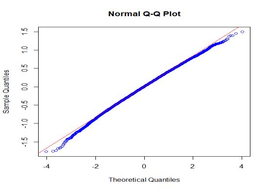
Normal Q-Q plot of EB predicted province
effects Histogram of residuals from the fitting of BHF
model to log (income + constant)
From the above graph, we can see that the
data set is going through the origin. So we can We see that it is approximately bell- shaped.
say that our observe data is normally That means data are normally distributed.
distributed.
Index plot of residuals from the fitting of BHF model to log (income + constant)
Above scatter plot indicates that the data are very closer to each other that means variance
are constant.
Figure 2: Checking model assumption12 Rahman et al.
Table 4: Comparison of Direct and Empirical Bayes (EB) estimates and their
respective coefficient of variation
Province Province Sample
Direct CV. DIR EB CV. EB
Index Name Size
1 Alava 96 0.255037 19.00367 0.335 7.226619
2 Albacete 173 0.140592 21.6384 0.159711 12.93839
3 Alicante 539 0.207851 10.48198 0.210909 5.402373
4 Almeria 198 0.26764 15.28299 0.24101 7.834946
5 Avila* 58 0.055122 46.35946 0.123793 24.96203
6 Badajoz 494 0.215539 10.93958 0.201012 5.96569
7 Baleares 634 0.099998 15.36549 0.11511 8.837025
8 Barcelona 1420 0.298125 5.428952 0.289218 2.307215
9 Burgos 168 0.214132 20.89156 0.188929 8.973926
10 Caceres 282 0.270313 11.56369 0.331773 4.358747
11 Cadiz 398 0.148874 14.7039 0.135251 8.6262
12 Castellon 118 0.175982 20.37073 0.255 8.938094
13 CiudadReal 250 0.209215 15.67395 0.20264 8.696991
14 Cordoba 224 0.299757 13.12423 0.311161 5.926287
15 CorunaLa 495 0.253475 9.73552 0.268444 3.99551
16 Cuenca 92 0.263341 22.45527 0.247717 9.927219
17 Gerona 142 0.183374 20.23291 0.222254 8.419048
18 Granada 208 0.317273 12.74599 0.335529 5.548515
19 Guadalajara 89 0.179082 23.64297 0.254157 9.667373
20 Guipuzcoa 285 0.236905 13.48546 0.245158 6.101039
21 Huelva 122 0.125834 25.45047 0.139508 16.48341
22 Huesca 115 0.241076 20.14448 0.278 8.05499
23 Jaen 232 0.312942 13.17392 0.284138 5.585637
24 Leon 218 0.188016 15.97012 0.249541 6.945103
25 Lerida 130 0.155596 24.88785 0.168231 12.96007
26 RiojaLa 510 0.258118 9.527405 0.265843 3.809543
27 Lugo 173 0.377187 15.10213 0.341387 5.242763
28 Madrid 944 0.182182 8.996593 0.191716 3.688254
29 Malaga 379 0.229185 11.93636 0.244908 5.155946
30 Murcia 885 0.177032 9.31421 0.186565 4.323254
31 Navarra 564 0.161908 11.37696 0.174574 5.835955
32 Orense 129 0.227996 18.41902 0.306667 7.349597
33 Oviedo 803 0.26064 8.03322 0.268319 3.274346
34 Palencia* 72 0.301661 23.80085 0.274306 11.25716
35 PalmasLas 472 0.166518 13.85587 0.150212 7.020753
36 Pontevedra 448 0.185491 13.04047 0.161652 7.475342
37 Salamanca 164 0.161045 18.61741 0.199634 10.25905
38 Tenerife 381 0.184296 11.14808 0.249711 4.648279Evaluating the Approaches of Small Area Estimation Using Poverty Mapping Data 13 39 Santander 434 0.342444 9.487491 0.351866 3.26399 40 Segovia* 58 0.22262 25.33449 0.283448 10.66742 41 Sevilla 482 0.20503 10.35226 0.231784 4.650448 42 Soria* 20 0.025412 99.97815 0.1175 42.7319 43 Tarragona 134 0.320354 15.40193 0.414328 5.333037 44 Teruel* 72 0.273642 24.57017 0.315556 9.257185 45 Toledo 275 0.125534 16.98341 0.149673 9.837353 46 Valencia 714 0.213607 9.693081 0.228852 3.890675 47 Valladolid 299 0.192923 16.64643 0.157492 9.689178 48 Vizcaya 524 0.216945 10.21295 0.22063 5.150919 49 Zamora 104 0.300274 20.06599 0.274712 8.936914 50 Zaragoza 564 0.100346 15.63731 0.112996 8.187835 51 Ceuta 235 0.197248 16.93905 0.189915 8.724863 52 Melilla 180 0.191091 18.00719 0.216833 7.904507 Above table shows that most of the estimated value of Direct estimation for each province less than the estimated value obtain by EB estimation. Coefficient of variation in each province for direct estimate is greater than the coefficient of variation (CV) of EB estimate. It can be visually shown in Figure 3 and Figure 4. *indicate 5 selected province with small sample size. The table shows that the estimated value of Direct (DIR) estimators for four provinces with small sample size namely Avila, Segovia, Soria, Teruel poverty incidence lie under EB estimates. Additionally that the differences are large in three provinces (Avila, Segovia, Soria), and are small in one of them (palencia). The above table also shows that the estimated C.Vs of Direct (DIR) for poverty incidence estimators are noticeably larger than those of Empirical Bayes (EB) estimators in all provinces. Such that we can say that EB estimate is better than direct estimation.
14                                                            Rahman et al.

                0.35
                0.25
     Estimate
                0.15
                0.05

                                              Direct
                                              EB

                       0       10      20       30       40         50
                           Area (sorted by decreasing sample size)

Figure 3: The estimated poverty incidence for Direct (DIR) and EB estimates

The figures above showed that most of the direct estimates for poverty incidence lie
under Empirical Bayes (EB) estimator for all selected provinces.
Evaluating the Approaches of Small Area Estimation Using Poverty Mapping Data 15
100
Direct
EB
Coefficient of variation (CV)
80
60
40
20
0
0 10 20 30 40 50
Province Code
Figure 4: Estimated C.Vs of Direct (DIR) and EB for each area
The above graph shows that the estimated C.Vs of Direct (DIR) estimators are
noticeably larger than those of Empirical Bayes (EB) estimators in all provinces.
From Figure 3 and Figure 4, it is clear that model based estimator such as Empirical
Bayes (EB) estimator is one of the most efficient estimator than direct estimator in
the case of small area estimation.16 Rahman et al.
0.4 0.4
Direct Estimates 0.35 0.35
SSD Estimates
0.3 0.3
0.25 0.25
0.2 0.2
0.15 0.15
0.1 0.1
0.05 0.05
0 0
0 500 1000 1500
0 500 1000 1500
Sample size Sample Size
0.3 0.5
Synthetic estimates
EB Estimates
0.25 0.4
Post-stratified
0.2
0.3
0.15
0.2
0.1
0.05 0.1
0 0
0 500 1000 1500 0 500 1000 1500
Sample Size Sample Size
Figure 5: Scatter plot of Direct, SSD, Post-stratified synthetic and EB
estimates according to sample size
From the Figure 5 it can be seen that scatter plot of direct estimates (Range:
0.025412-0.377187), SSD estimates (Range: .100346-.375823) and EB estimates
(Range: 0.11299-0.41432) according to the sample size estimated value are
fluctuately increasing as sample size increases, they are unstable (Range: 0.025412-
0.377187) and they are approximately same. But in the case of post-stratified
synthetic estimated values are stable (Range: 0.202825-0.261705). Comparing to
the direct estimates with indirect estimates (post-stratified synthetic, SSD, EB) it
can be shown that the estimated value of indirect estimates are greater than direct
estimated values as if there is small sample size.Evaluating the Approaches of Small Area Estimation Using Poverty Mapping Data 17
o EB Estimates
- Mean value
0.35
EB Estimate
0.25
0.15
0 10 20 30 40 50
Province Code
Figure 6: Scatter plot of Direct, post-stratified synthetic, SSD and EB
estimates according to province code
Figure 6 indicates that the estimated value of Direct, SSD and EB estimator have a
great distance from their mean value and the estimated value of Post-stratified
Synthetic estimator are closer to their mean value and they are approximately stable.18 Rahman et al.
0.5 0.4
0.4
True values
0.3
True values
0.3
0.2
0.2
0.1 0.1
0 0
0 0.2 0.4 0.6 0 0.2 0.4 0.6
Direct estimates Post-stratified synthetic estimates
OLS regression line Y=X line OLS regression line Y=X line
0.4 0.5
0.3 0.4
True value
True value
0.2 0.3
0.2
0.1
0.1
0
0 0.2 0.4 0.6 0
0 0.2 0.4 0.6
Saple size dependent (SSD)
estimate Emperical Bayes (EB) estimate
OLS regression line Y=X line OLS regression line Y=X line
Figure 7: Bias scatter plot between True values and Direct, post-stratified
synthetic and EB estimates
The scatter plot of true value (on the Y-axis) against direct estimates and EB
estimates (on the X-axis) displayed a regression line close to the Y=X line. Here the
slope coefficient estimate was near to 1 and intercept was not significantly differ
from zero (0), indicating that there is no evidence to reject the hypothesis of lack
bias for the direct estimate. That means, it can be conclude that Direct estimates and
EB estimates are approximately unbiased. The main difference is that the value
points in EB estimator are situated exactly in a straight line but the points of direct
estimator have a significance distance from the straight line.
The scatter plot of true value (on the Y-axis) against post-stratified synthetic
estimates and SSD estimates (on the X-axis) displayed a regression line that are not
close to the Y=X line. Here the slope coefficient estimate was not near to 1 and
intercept was significantly differ from zero (0), indicating that there is an evidenceEvaluating the Approaches of Small Area Estimation Using Poverty Mapping Data 19 to reject the hypothesis of lack bias for the post-stratified synthetic estimate. That means, it can be conclude that post-stratified synthetic estimates and SSD estimates are extreme biased. 5. Conclusion Our estimated results shown that direct estimates and sample size dependent (SSD) estimates are very similar. The estimated value of these two methods are fluctuately decreases as sample size decreases and they are slightly more unstable. It is noticeable that when sample size is large the SSD estimator treated as a direct estimator, but it is increases when sample size was small. However, the post- stratified synthetic estimates appear to be too stable, giving practically the same values for all provinces. But direct estimator is approximately unbiased but SSD and Post-stratified synthetic estimator is extreme biased. EB estimator depicted that most of the estimated value of Direct estimation for each province less than the estimated value obtain by EB estimation. Coefficient of variation in each province for direct estimate is greater than the coefficient of variation (CV) of EB estimate and it can also be shown that EB estimator is approximately unbiased. Such that we can say that EB (model based) estimate is better estimation method in the case of small area estimation. That's why, it is impossible to think any research work without knowing the SAE technique in the present world.
20                                                              Rahman et al.

References
[1] Arora, V. and Lahiri, P. (1997). On the superiority of the Bayesian method
     over the BLUP in small area estimation problems. Statistica Sinica, 7, 1053-
     1063.
[2] Rahmn, A. (2008). A Review of Small Area Estimation Problems and
     Methodological Developments. Australia. NATSEM, University of Canberra.
[3] Chandra, H., Aditya, K. & Sud, U. C. (2018). Localised estimates and spatial
     mapping of poverty incidence in the state of Bihar in India - An application of
     small area estimation techniques. PLoS ONE, 13, 6, e0198502.
[4] Datta, G. S., Rao, J. N. K. and Smith, D. D. (2005). On measuring the
     variability of small area estimators under a basic area level model. Biometrika,
     92,1, 183–196.
[5] Drew, D., Singh, M.P. & Choudhry, G.H. (1982). Evaluation of small area
     estimation techniques for the Canadian Labour Force Survey. Survey
     Methodology, 8, 17-47.
[6] Drew, D., Singh, M.P. and Choudhry, G.H. (1982). Evaluation of small area
     estimation techniques for the Canadian Labour Force Survey. Survey
     Methodology, 8, 17-47.
[7] El-Yasha, S. R., Rizky, M., Wibowo, T. W. & Sudaryatno, (2019). Spatial
     Analysis of Poverty and Happiness Profiles in Special Region of Yogyakarta
     Using Small Area Estimation Method. The International Archives of the
     Photogrammetry, Remote Sensing and Spatial Information Sciences, Volume
     XLII-4/W16.
[8] European Commission. "Small Area Methods for Poverty and Living
     Condition Estimates Project", http://www.sample-project.eu/.
[9] Ghosh, M. & Rao, J.N.K. (1994). Small area estimation: an appraisal.
     Statistical Science, 9, 55-93.
[10] Kamal El Saied, M. M., Talat, A. A. and El Gohary, M. M. (2019). Small
     Area Procedures for Estimating Income and Poverty in Egypt. Asian Journal
     of Probability and Statistics, 4, 1, 1-17.
[11] Marchetti, S., Giusti, C., Pratesi1, M. Salvati, N., Giannotti, F., Pedreschi, D.,
     Rinzivillo, S., Pappalardo, L., and Gabrielli, L. (2015). Small Area Model-
     Based Estimators Using Big Data Sources. Journal of Official Statistics, 31, 2,
     263–281. http://dx.doi.org/10.1515/JOS-2015-0017
[12] Molina, I. & Marhuenda, Y. (1982). sae: An R package for Small Area
     Estimation. R Journal, Under revision.
[13] Molina, I. and Marhuenda, Y. (2015). sae: An R Package for Small Area
     Estimation. The R Journal Vol. 7/1.
[14] Nájera Catalán, H.E., Fifita, V.K. and Faingaanuku, W. (2020). Small-Area
     Multidimensional Poverty Estimates for Tonga 2016. Drawn from a
     Hierarchical Bayesian Estimator. Appl. Spatial Analysis 13, 305–328.
     https://doi.org/10.1007/s12061-019-09304-8
Evaluating the Approaches of Small Area Estimation Using Poverty Mapping Data 21
[15] Pusponegoro, N. H. and Rachmawati, R. N. (2018). Spatial Empirical Best
Linear Unbiased Prediction in Small Area Estimation of Poverty.
Science Direct, 135, 712–718.
[16] Pusponegoro, N. H., Djuraidah, A., Fitrianto A. and Sumertajaya, I. M. (2019).
Geo-additive Models in Small Area Estimation of Poverty. Journal of Data
Science and Its Applications, 2, 1, 11-18.
[17] Rao, J. N. K. and Molina, I. (2015). Small area estimation 2nd edition. New
Jersey, John Wiley & Sons.
[18] Rao, J.N.K. (2003). Small Area Estimation. Wiley, London.
[19] Suhartini T., Sadik, K. and Indahwati, (2016). Small area estimation (SAE)
model: Case study of poverty in West Java Province. AIP Conference
Proceedings 1707, 080016. https://doi.org/10.1063/1.4940873
[20] Sundara, V. Y., Kurnia, A. and Sadik, K. (2017). Clustering Information of
Non-Sampled Area in Small Area Estimation of Poverty Indicators. IOP
Conference Series: Earth and Environmental Science, 58, 012020.
https://doi.org/10.1088/1755-1315/58/1/012020
[21] Szymkowiak, M., Młodak, A. and Wawrowski, L. (2017). Mapping Poverty at
the Level of Subregions in Poland Using Indirect Estimation. STATISTICS IN
TRANSITION new series, 18, 4, 609–635.
[22] You, Y. and Chapman, B. (2006). Small area estimation using area level
models and estimated sampling variances. Survey Methodology, 32, 97-103.You can also read