Flood Detection Using Multi-Modal and Multi-Temporal Images: A Comparative Study - MDPI
←
→
Page content transcription
If your browser does not render page correctly, please read the page content below
remote sensing
Technical Note
Flood Detection Using Multi-Modal and
Multi-Temporal Images: A Comparative Study
Kazi Aminul Islam 1 , Mohammad Shahab Uddin 1 , Chiman Kwan 2                    and Jiang Li 1, *
 1    Department of Electrical & Computer Engineering, Old Dominion University, Norfolk, VA 23529, USA;
      kisla001@odu.edu (K.A.I.); muddi003@odu.edu (M.S.U.)
 2    Applied Research LLC, Rockville, MD 20850, USA; chiman.kwan@arllc.net
 *    Correspondence: jli@odu.edu

 Received: 29 June 2020; Accepted: 28 July 2020; Published: 30 July 2020

 Abstract: Natural disasters such as flooding can severely affect human life and property. To provide
 rescue through an emergency response team, we need an accurate flooding assessment of the
 affected area after the event. Traditionally, it requires a lot of human resources to obtain an accurate
 estimation of a flooded area. In this paper, we compared several traditional machine-learning
 approaches for flood detection including multi-layer perceptron (MLP), support vector machine
 (SVM), deep convolutional neural network (DCNN) with recent domain adaptation-based approaches,
 based on a multi-modal and multi-temporal image dataset. Specifically, we used SPOT-5 and RADAR
 images from the flood event that occurred in November 2000 in Gloucester, UK. Experimental results
 show that the domain adaptation-based approach, semi-supervised domain adaptation (SSDA) with
 20 labeled data samples, achieved slightly better values of the area under the precision-recall (PR)
 curve (AUC) of 0.9173 and F1 score of 0.8846 than those by traditional machine approaches. However,
 SSDA required much less labor for ground-truth labeling and should be recommended in practice.

 Keywords: flood detection; deep convolutional neural network; domain adaptation; SVM; MLP

1. Introduction
      Flooding is one of the most severe forms of natural disasters. It affected all over the world and
caused millions of human deaths [1,2]. Flooding is the second deadliest natural disaster in the United
States and hurricanes Katrina, Mathews, Florence and Sandy caused severe property damages and
thousands of lives were lost [3]. To mitigate the damage of flooding, an early accurate estimation of
the flooded area is a necessary step for a rescue team to help the people in the affected area.
      Throughout the years, researchers developed automatic methods to monitor flood events using
remote sensing data. Automatic methods are quick, cost-effective, and monitoring from distance as
compared to traditional methods, which require labor, in-person visit and longer processing time.
In remote sensing domain, wide range of sensors are available. Some provide better spatial resolutions
and others provide more frequent temporal revisit. Remote sensing-based flood-detection methods
can be divided into two categories: optical and radar sensor. Optical data such as WorldView2 [4],
Landsat [5–7], Spot-5 [8], sentinel [9], Moderate-Resolution Imaging Spectroradiometer (MODIS) [7,10]
and RADAR [8,11–13] had been explored for flood detection. In the meanwhile, machine-learning
algorithms including decision tree algorithm [4,14], SVM [6,8], MLP [8] had been developed for
flood detection.
      The data fusion technical committee (DFTC) of the IEEE Geo-Science and Remote Sensing Society
organized a contest to perform flood detection using a multi-temporal and multi-modal dataset in
2009 [8]. This dataset contains SPOT-5 satellite images and radar images from both the pre- and
post-flooding event occurred in 2000 in Gloucester, UK. In the contest, traditional machine-learning

Remote Sens. 2020, 12, 2455; doi:10.3390/rs12152455                        www.mdpi.com/journal/remotesensing
Remote Sens. 2020, 12, 2455                                                                          2 of 17

methods including SVM and MLP were winners in the supervised flood-detection scenario. The SVM
model used the SPOT-5 satellite images combined with four derived morphological channels from
the near infrared (NIR) channel in the original data for flood detection. The MLP model used both
the SPOT-5 satellite and radar images. Both the MLP and SVM methods concatenated the pre- and
post-event flooding data in training and testing and the two models provided similar performance [8].
Liu et al. introduced a homogeneous pixel transformation algorithm [15] to detect flood using the
same DFTC dataset [8].
     Deep Learning is a subset of machine-learning techniques. We called the machine-learning model
as a deep learning model when we use multiple layers of neural network. Deep learning model has
been used in wide range of applications including computer vision [16–18], speech-based medical
diagnosis [19,20], cybersecurity [21,22], medical disease diagnosis [19,23], remote sensing [17,24,25]
domains. To train a deep learning model from a scratch, we usually need a lot of labeled data because
deep learning models contain a large number of trainable parameters. This usually posts a challenge
in practice because it is not always possible to collect sufficient labeled data for training. To solve this
problem, one possible solution is to fine-tune a pre-trained model with limited available labeled data.
Examples can be found in biomedical application [26], facial expression recognition [27] and plant
recognition [28].
     Flood detection attracted significant amount of attention after the competition and new datasets
and deep learning algorithms had been developed for this purpose. Deep learning algorithms such as
deep neural network [29], deep convolutional neural network (DCNN) [30,31] and fully convolutional
neural networks (F-CNNs) [32] with satellite images including Sentinel-2 [30], Planet [31], Landsat [32]
and Google Earth aerial imagery [29] have been used for flood detection. Unmanned aerial vehicles
(UAV) image data with VGG-based fully convolutional network (FCN-16s) was also developed for
flood detection [33].
     Most of the flood-detection methods including the winners of the competition concatenated both
the pre- and post-event images for training [8]. For example, the ground-truth of region of interest
(ROI) in the competition were defined by examining both the pre- and post-event images and flood
and non-flooded regions were identified as ground-truth ROIs for training. However, it is not always
possible to obtain ground truth after the flood event in practice, making the developed methods
challenging to be applied in practice.
     An alternative is to train a model using ROIs defined on pre-event images and directly apply
the trained model to post-event images for flood detection. However, models trained in one domain
usually cannot perform well in another domain if there are data distribution shifts between the two
domains, and there is a need to incorporate domain adaptation techniques to address the distribution
shift challenge. For example, if we train a classifier using the ground truths defined in pre-event
images and use the trained classifier directly to detect flood in post-event images, our experimental
results on the competition dataset showed that the performances dropped significantly.
     To address this issue, researchers have developed many domain adaptation approaches among
which the generative adversarial network (GAN) [34]-based approaches have been very popular for
image classification and segmentation. Tzeng et al. used a GAN loss to mimic the target domain to
represent the source domain [35]. Motiian et al. used a Siamese architecture where they used a few
samples to adapt a model into different domain [36]. Our previous study used a semi-supervised
domain adaptation approach for seagrass detection and achieved better results in seagrass detection
as compared with other methods [18].
     The motivation of this study is to perform a comparative study on the various domain adaptation
algorithms with those competition winners for flood detection on the competition dataset, and provide
useful practical suggestions for flood detection. Contributions of this paper are:

•     We implemented domain adaptation methods and compared these methods with traditional
      machine-learning algorithms for flood detection. To the best of our knowledge, we are the first to
      implement a deep learning-based domain adaptation approach for flood detection.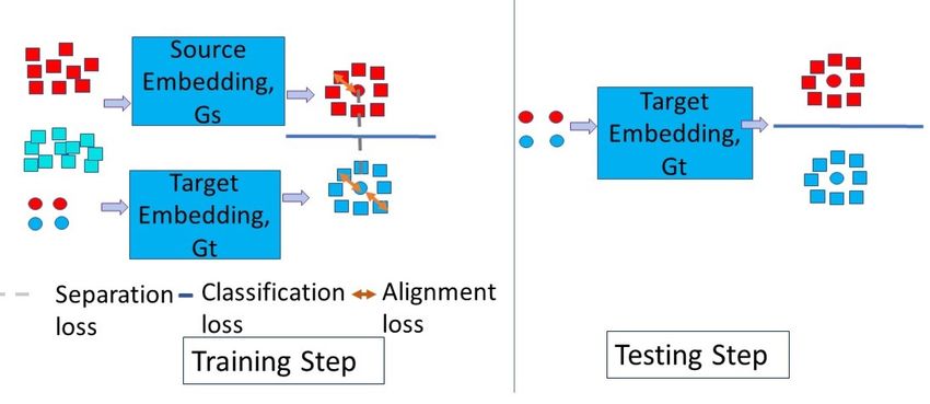
Remote Sens. 2020, 12, 2455                                                                              3 of 17

•     Our experimental results showed that domain adaptation-based methods can achieve competitive
      performance for flood detection and require much less labeled samples in the post-event images
      for model fine-tuning.
•     Our recommendation for the community is that domain adaptation methods require less labor
      and are better tools for flood detection.

     The paper is structured as follows: Section 2 describes data and experiment design.
Sections 3 and 4 present results and discussions, respectively, and Section 5 summarizes the paper.

2. Dataset and Experiment Design

2.1. Dataset
     We used two heterogeneous satellite image sensors including SPOT-5 and a European Remote
Sensing 1 (ERS-1) SAR images as shown in Figure 1 from the competition [8]. The images were
captured from the flooding event occurred in November 2000 in Gloucester, UK. The SPOT-5 optical
sensor image contains three bands including Red, Green, and Near-inferred-1 and radar image only
contains the SAR channel. The green, red and near IR channels have spectral ranges of 0.50–0.60 µm,
0.61–0.68 µm, and 0.78–0.89 µm, respectively, with 20 m spatial resolution. The SAR image uses C-band,
5 GHZ frequency with linear VV polarization. The SAR images also use wave mode to collect the
temporal images with a spatial resolution of 10 m and a swath width of 5 km.
     The pre-event and post-event images are shown in Figure 1. Two temporal images of SPOT-5 are
taken in September 2000 and November 2000 as shown in Figure 1a,c. The pre-event and post-event of
SAR images are taken in October 2000 and November 2000 as displayed in Figure 1b,d, respectively.
The original ground truth provided by the organizers were found to be inaccurate and we used the
updated ground truth [15] in our study as shown in Figure 2b. For the SAR image, we took a logarithm
operation on the pixel values and applied a de-speckle filtering process with a 7 × 7 window to
improve its resolution.

    (a) Pre-event SPOT image (b) Pre-event SAR Image (c) Post-event SPOT Image (d) Post-event SAR Image

      Figure 1. Multi-modal and multi-temporal Images taken in Gloucester, UK. Spot-5 images are displayed
      using Green, Red and NiR Band.

2.2. Data Augmentation with Morphological Operation
    Some winners of the competition augmented the data with morphological operation. For a fair
comparison, we also created four additional bands using morphological operation as described in [8].
We used opening by reconstruction (OR) operation on the NIR band with a circular structuring element
radius of 40 and 100. In addition, we implemented closing by reconstruction (CR) operation on the
images resulted from the last step with a circular structuring element radius of 60 and 90. In total,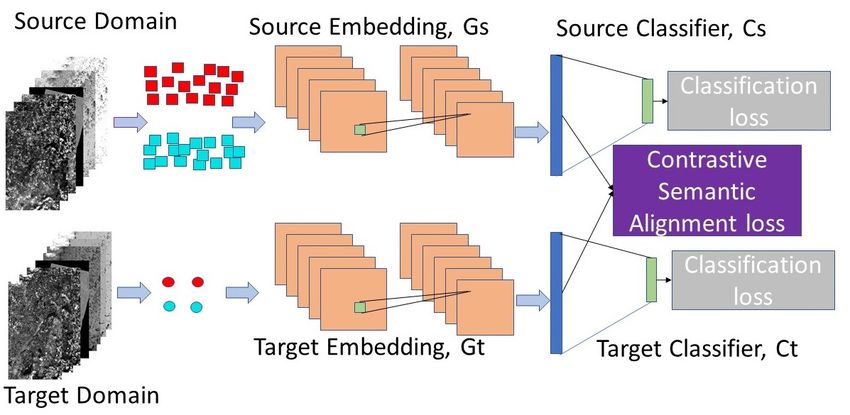
Remote Sens. 2020, 12, 2455                                                                             4 of 17

we created four additional bands based on the original images. The created four bands for the pre-event
and post-event image are shown in Figure 3.

                              (a)                                               (b)

      Figure 2. Ground Truth. (a) Selected ROIs in the pre-event image; (b) Updated flooding ground truth
      in the post-event image [15].

           (a) OR 40                 (b) CR 60                 (c) OR 100                  (d) CR 90

           (e) OR 40                 (f) CR 60                 (g) OR 100                  (h) CR 90

      Figure 3. Derived morphological bands based on the pre-event (1st row) and post-event (2nd row)
      SPOT-5 image’s NIR band. CR: Closing by Reconstruction. OR: Opening by Reconstruction.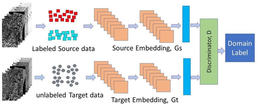
Remote Sens. 2020, 12, 2455                                                                                             5 of 17

2.3. Models for Comparison

2.3.1. Multi-Layer Perceptron (MLP)
     Multi-layer Perceptron (MLP) is also known as feed-forward artificial neural network (ANN)
uses a perceptron algorithm to perform tasks. Geoffrey Hinton et al. introduced a back-propagation
algorithm [37] which made the MLP algorithm effective and widely popular among researchers.
The back-propagation algorithm adjusts the weights of the MLP model to minimize the difference
between the actual output and the desired output [37]. MLP usually uses three layers of network
to perform classification and regression tasks. MLP algorithm has been effectively used for flood
detection by the winners of the competition [8].
     We re-implemented the MLP classifier that achieved the best performance in the data fusion
contest [8]. This model stacked the SPOT-5 and radar images from both the pre-event (t1) and
                                                                                t     t      t        t1
post-event (t2) for flood detection. The stacked data consists of 8 bands as [ XR1 , XG1 , X N1 IR , XSAR , XRt2 ,
  t2   t2      t2
XG , X N IR , XSAR ]. The model was trained using the labeled regions of interest (ROIs) in both the t1
and t2 images and then was applied to the whole images for flood detection. The architecture of the
MLP model is shown in Figure 4.

                                     Figure 4. Multi-layer Perceptron Architecture.

2.3.2. Support Vector Machine (SVM)
      Support Vector Machine [38] is another popular machine-learning method which has been
widely used for classification and is considered to be a baseline for image classification. SVM finds
hyper-planes among data points as classification boundaries. Linear, polynomial, Gaussian radial
basis function, and Hyperbolic tangent kernel is generally used for SVM classification. LIBSVM [39] is
a popular implementation for SVM models.
      We followed the same settings of another winner in the competition who used an SVM classifier
for flood detection [8]. This model used the four additional bands created by morphological operation
on the NIR band in the post-event’s SPOT image as described in Section 2.2, making the input
                      t   t      t
data 10 bands as [ XR1 , XG1 , X N1 IR , XRt2 , XG
                                                 t2    t2
                                                    , XN         t2           t2            t2           t2
                                                          IR , X N IROR40 , X N IROR100 , X N IRCR60 , X N IRCR90 ]. Similarly,
the model was trained using the labeled ROIs in both the t1 and t2 images and then was applied to the
whole images for flood detection.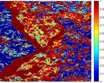
Remote Sens. 2020, 12, 2455                                                                                          6 of 17

2.3.3. Source Only (SO)
      To compare with the domain adaptation-based flood-detection methods, we treated the pre-event
images as source domain and the post-event as target domain. The SO method is the baseline model,
in which we trained a classifier (CNN/MLP/SVM) only using the ROIs labeled in the pre-event images.
We then directly applied the trained classifier to the post-event images for flood detection.
      In source only models, we only used the pre-event image’s ROIs to learn the difference between
the flood and non-flood data without using any labeled and unlabeled data from the post-event images.
The CNN-SO model’s architecture is shown in Figure 5. Here, the DCNN model has two convolutional
layers and two fully connected layers. The convolutional layers use filters to search for task-specific
features in the images. If it finds similar features present in the images, the filters produce a high
agreement. Initially, the filters are random but after a few iterations, the filters are optimized to scan
task-specific features. After two convolutional layers, we used a fully connected layer as shown in
Figure 5. The fully connected layer works similarly to the MLP model. The last layer performs the
classification task and predicts the probability of being flood class or non-flood class.

                              Figure 5. Deep Convolutional Neural Network Architecture.

      We stacked the images as [XRt1 , XG    t1 , X t1 , X t1 , X t1
                                                    N IR    SAR     N IROR40
                                                                             , XN t1
                                                                                     IROR100
                                                                                                t1
                                                                                             , XN  IRCR60
                                                                                                             t1
                                                                                                          , XN  IRCR90
                                                                                                                       ] for
                  t2   t2   t2     t2      t2            t2           t2           t2
training, and [XR , XG , X N IR , XSAR , X N IROR40 , X N IROR100 , X N IRCR60 , X N IRCR90 ] for flood detection. We
normalized the data between 0 to 1 in each band and used the labeled ROIs in the pre-event images
for training, no label information in the post-event images were used during training. All subsequent
methods described in Sections 2.3.4–2.3.7 used the same data composition.

2.3.4. Unsupervised Domain Adaptation (UDA)
     Unsupervised domain adaptation based on generative adversarial network (GAN) [35] became
popular since GAN was created in 2014 [34], and we implemented the approach proposed for flood
detection. First, we trained a deep convolutional neural network (DCNN) model in the source domain
using all the labeled ROIs. After the training, the DCNN model learned the source embedding function,
Gs and source classifier Cs for flood detection (Figure 6a). In the second step, we used the unlabeled
data from both the source and target domains to match the marginal distribution between the source
(P( GS ( X s ))) and the target domains (P( Gt ( X t ))) based on the GAN loss (Figure 6b). The target
embedding was trained to represent the source embedding so that the classifier trained on the source
domain was used in the target domain for flood detection.
     Let the source and target domain datasets to be denoted as Ds = { X s ,Y s } and Dt = { X t },
respectively. First, we train a DCNN model using the labeled samples from the source domain
(Figure 6a),
                                         Lc ( f s ) = E[l ( f s ( X s ), Y s )]                     (1)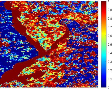
Remote Sens. 2020, 12, 2455                                                                                            7 of 17

where f s is the DCNN model and E is the expectation function and l is any related loss functions.
f s can be divided into two function source embedding function, Gs and source classifier, Cs . We use
the trained source embedding function Gs to find an optimum target embedding function Gt using the
unlabeled data from both domains. We modify the target domain Gt using a GAN loss to match the
source domain embedding function Gs . The discriminator, D, in Figure 6b is trained using following
GAN loss,

                L advD ( X s , X t , Gs , Gt ) = Exs ∼X s [logD ( Gs ( x s ))] − Ext ∼X t [log(1 − D ( Gt ( x t )))]      (2)

      The target embedding function Gt uses the following generator loss to mimic the source domain,

                                 MinGt L advG ( X s , X t , D ) = − Ext ∼X t [logD ( Gt ( x t ))]                         (3)

   Using this feedback, the target embedding function Gt modifies its parameter so that the source
domain classifier can work on the target domain.

2.3.5. Semi-Supervised Domain Adaptation (SSDA)
     We modified our previous work [18] for flood detection as shown in Figure 6. First, a DCNN
model was trained using the source domain labeled ROIs. After training, the source embedding
function was first adapted to target domain using UDA described in Section 2.3.4. Then, a few labeled
samples from the target domain were used to align the class-specific distribution between the source
and the target domain based on the semantic contrastive alignment and classification loss (CSA)
(Figure 6c). The CSA loss put the same class samples from different domains together and different
class samples from the different domains as far as possible (Figure 6d).
     To reduce the classwise distribution shift between the source and target domain, we used a few
labeled samples from the target domain Dt = { X t , Y t } with the classification and contrastive semantic
alignment loss (CCSA) [18,36]. The classification loss was defined as,

                                                LC ( G ◦ C ) = E[l ( f ( X ), Y )]                                        (4)

    The contrastive semantic alignment (CSA) loss consists of semantic alignment loss and class
separation loss,
                                 LCSA ( G ) = LSA ( Gt ) + LCS ( Gt )                       (5)

where LSA ( Gt ) is the semantic alignment loss and LCS ( Gt ) is the class separation loss. LSA ( Gt ) is
computed as,
                                                       Nc
                                       LSA ( Gt ) =    ∑ d( p(Gs (Xas )), p(Gt (Xat )))                                   (6)
                                                      a =1

where Nc is the number of classes, Xas = X s /{Y = a} and Xat = X t /{Y = a} are conditional random
variables and d is a distance metric between source Xas and target Xat distributions.
     We used the semantic alignment loss to map samples from the same class from source domain and
target as close as possible. We also used the following class separation loss to map samples carrying
different class labels from different domains as far as possible in the embedding space,

                                     LCS ( Gt ) =      ∑        k( p( Gs ( Xas )), p( Gt ( Xbt )))                        (7)
                                                    a,b| a6=b

where k denotes the similarity matrix. If the distributions of Xas and Xbt are close to each other the
loss function puts a penalty to keep them separate. Figure 6d represents the working procedure of
the CSA loss. The semantic alignment, class separation and classification loss are represented as the
orange arrows, red dashed line and blue solid line, respectively. During testing, we used the trained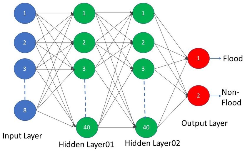
Remote Sens. 2020, 12, 2455                                                                            8 of 17

target mapping function, Gt , to find the new representation. The overall classification and contrastive
semantic alignment loss becomes,

                                LCCSA ( Gt ) = LC ( Gt ◦ Ct ) + LSA ( Gt ) + LCS ( Gt )                   (8)

                                (a) Source domain supervised DCNN model training

       (b) Target domain embedding function learned using unsupervised adversarial domain adaptation

                              (c) Target domain supervised adaptation using CCSA loss

                          (d) Training and testing steps of CCSA loss using labeled samples

                 Figure 6. Semi-supervised domain adaptation (SSDA) method for flood detection.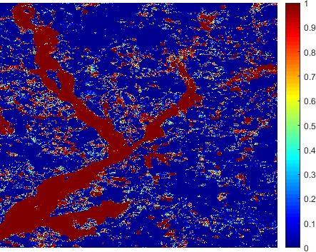
Remote Sens. 2020, 12, 2455                                                                          9 of 17

2.3.6. SVM, MLP and DCNN Fine-Tuned with 1, 3, 5, 10, and 20 Samples/Shots
     First, we used the labeled ROIs in the pre-event images to train the classifiers (SVM/MLP/DCNN).
Then, we used 1, 3, 5, and 20 labeled samples from the post-event images to fine-tune the classifiers.
The fine-tuned classifiers were applied to classify the post-event images.

2.3.7. MLP and SVM with 20 Samples from Post-Event Images
      We combined the ROIs in the pre-event images with 20 labeled samples from ROIs in the
post-event images to train the SVM and the MLP classifiers. After training, we used trained classifiers
for flood detection. In other domain adaptation methods, the pre-event image ROIs were used for
training and a few labeled samples from post-event images were used to adapt the trained model to
detect flood in target domain. This experiment was conducted to test if the sequential use of pre- and
post-event labeled samples can provide any advantage.

2.4. Evaluation Metrics
      Our dataset contains much more non-flooded pixels than flooded ones and is highly imbalanced.
It was found that for binary imbalanced dataset, the precision-recall (PR) curve is a good performance
metric to assess effectiveness of different classification models [40,41]. The area under the PR
curve (AUC) is also computed as a performance metric. In addition, we apply 0.5 as threshold
to flood-detection probability maps to obtain the final detections, which are used to compute precision,
recall and F1 score metrics for different models as follows.
                                             # o f true f lood pixels detected
                               Precision =                                                              (9)
                                                # o f total pixels detected

                                           # o f true f lood pixels detected
                                Recall =                                                              (10)
                                           # o f total labeled f lood pixels
                                                  2 ∗ Precision ∗ Recall
                                   F1 − score =                                                       (11)
                                                    Precision + Recall

2.5. Hyper-Parameter Determination
     We selected a patch-size of 5 × 5 in our experiments after considering the trade-off between
performance and computational time. In the SSDA method, 10,000 labeled samples from each class in
the source domain were randomly selected to pair with a few labeled samples in the target domain for
adaptation. For the embedding functions in source domain, Gs and target domain, Gt , we used two
convolutional layers followed by a flatten layer as embedding functions. The first layer had 25 filters
with a size of 2 × 2 × 8 and the second layer had 25 filters with a size of 4 × 4 × 20. All layers used the
ReLu activation function. Both classifiers, Cs and Ct in CNN models contained a fully connected layer
with 25 hidden units. The output layer had 2 units with SoftMax activation function for classification.
We trained the source CNN models for 200 epochs with a batch size of 128. We trained the UDA step
for 300 epochs and the SSDA step for 240 epochs in all experiments. We followed similar settings of
the competition [8] and used an SVM classifier from the scikit-learn library [42] with a linear kernel.
The SVM was implemented based on libsvm [39]. We use a grid search optimization technique to
optimize the SVM classifier’s parameters. We perform a grid search among linear and RBF kernels,
C parameters between 1 to 1000 and Gamma value between 1 × 10⁻³ and 1 × 10⁻⁴ . Similarly, the MLP
classifier had two hidden layers with 40 hidden unites each.

3. Results
     In Table 1, the classification performances of SVM source only (SO), MLP SO, and DCNN SO
methods are shown in the first three rows. The unsupervised domain adaptation results are shown in
the fourth row in Table 1. Row 5 to row 23 are results by 1-shot, 3-shot, 5-shot, 10-shot, and 20-shot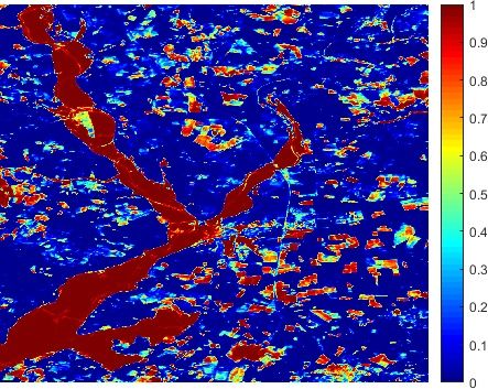
Remote Sens. 2020, 12, 2455                                                                                   10 of 17

from the post-event images with MLP fine-tuning (FT), SVM FT, DCNN FT, and Semi-supervised
domain adaptation (SSDA) approaches. The last two rows show results by the two winners: MLP [8]
and SVM [8] in the flood-detection competition.

      Table 1. Performance comparison. Precision, Recall, and F-1 score are calculated using 0.5 as threshold,
      and the area under the PR curve (AUC) values are computed on the OPP and MO-DS images. OPP:
      Original predication probability. MO-DS: Morphological operation with a disk structure.

                                    Recall           Precision            F1-Score             PR-AUC
           Methods
                              OPP      MO-DS     OPP      MO-DS       OPP      MO-DS       OPP      MO-DS
          SVM-SO              0.9761    0.9740   0.1950    0.2108    0.3251     0.3466    0.7904     0.8132
          MLP-SO                 0         0        0         0       NA         NA       0.2032     0.2203
          CNN-SO              0.8853    0.8571   0.3653    0.4201    0.5172     0.5638    0.7681     0.8070
           UDA                0.8764    0.8554   0.8246    0.8754    0.8497     0.8652    0.8508     0.8833
         MLP 20 shots         0.9007    0.8593   0.2017    0.2206    0.3295     0.3510    0.2460     0.2605
       DCNN 1-shot FT         0.8076    0.7757   0.5683    0.6201     0.6671    0.6892    0.8281     0.8524
        MLP 1-shot FT         0.9311    0.9279   0.4871    0.5305     0.6396    0.6751    0.7900     0.8617
        SVM 1-shot FT         0.0723    0.0654   0.0115    0.0105     0.0199    0.0181    0.0485     0.0484
         SSDA 1-shot          0.8407    0.8111   0.8623    0.8972     0.8513    0.8520    0.7155     0.8433
       DCNN 3-shot FT         0.8699    0.8514   0.7772    0.8259     0.8209    0.8385    0.7783     0.8115
        MLP 3-shot FT         0.9168    0.9118   0.6045    0.6539     0.7286    0.7616    0.8470     0.8829
        SVM 3-shot FT         0.9092    0.9023   0.7182    0.7631     0.8025    0.8269    0.8780     0.8969
         SSDA 3-shot          0.9341    0.9306   0.5409    0.5899     0.6851    0.7221    0.8906     0.9062
       DCNN 5-shot FT         0.7934    0.7600   0.8975    0.9261     0.8422    0.8349    0.8349     0.8577
        MLP 5-shot FT         0.8404    0.8199   0.8765    0.9055     0.8580    0.8605    0.8910     0.9064
        SVM 5-shot FT         0.8792    0.8650   0.8244    0.8614     0.8509    0.8632    0.8797     0.8984
         SSDA 5-shot          0.8493    0.8216   0.8989    0.9293     0.8734    0.8721    0.8209     0.8901
      DCNN 10-shot FT         0.8349    0.8088   0.8635    0.9004     0.8490    0.8521    0.8163     0.8439
       MLP 10-shot FT         0.8505    0.8313   0.8515    0.8862     0.8510    0.8578    0.8813     0.9019
       SVM 10-shot FT         0.8720    0.8562   0.8460    0.8798     0.8588    0.8678    0.8820     0.8998
        SSDA 10-shot          0.8750    0.8518   0.8515    0.9027     0.8631    0.8765    0.8506     0.9035
      DCNN 20-shot FT         0.8812    0.8619   0.7472    0.8317     0.8087    0.8466    0.8663     0.8925
       MLP 20-shot FT         0.8756    0.8502   0.7879    0.8465     0.8294    0.8484    0.8194     0.8966
       SVM 20-shot FT         0.8901    0.8704   0.8012    0.8566     0.8433    0.8634    0.8532     0.8960
        SSDA 20-shot          0.8831    0.8704   0.8681    0.8992     0.8755    0.8846    0.8669     0.9173
            SVM [8]           0.9393    0.9333   0.6263    0.7126    0.7515     0.8082    0.8442     0.8727
            MLP [8]           0.9406    0.9287   0.5472    0.7139    0.6919     0.8073    0.8567     0.8949

Original Predicted Probability (OPP) Results
     Each method produced a flooding probability map and we computed Precision, Recall and
F1-score on the thresholded original maps for comparison, shown as ‘OPP’ in Table 1. We also
compare the PR-AUC values to evaluate the flood-detection performance of each method. The OPP
maps for different models are shown in Figure 7. We use a ‘jet’ color-map (Matlab) to show the
flood-detection probability for each method. Color blue represents the probability ‘0’ and color red
represents probability ‘1’. Also, we add a color-bar to display different probability values. The PR
curves for the last six flood-detection scenarios in Table 1 are shown in Figure 8a.
Remote Sens. 2020, 12, 2455 11 of 17
(a) CNN-SO (b) MLP SO (c) SVM-SO (d) UDA
(e) SVM 1-shot FT (f) SVM 20-shot FT (g) MLP 1-shot FT (h) MLP 20-shot FT
(i) DCNN 1-shot FT (j) DCNN 20-shot FT (k) SSDA 1-shot (l) SSDA 20-shot
(m) SVM [8] (n) MLP [8]
Figure 7. Original predicted probability (OPP) maps. Blue represents the probability ‘0’ and Red
represents probability ‘1’.Remote Sens. 2020, 12, 2455 12 of 17
PR Curves for Prediction Map
1
0.95
0.9
0.85
0.8
Precision
0.75
0.7
0.65
MLP[longbotham et al]
SVM[longbotham et al]
0.6 SSDA 20 shots
MLP 20 shots FT
0.55 SVM 20 shots FT
DCNN 20 shots FT
0.5
0 0.1 0.2 0.3 0.4 0.5 0.6 0.7 0.8 0.9 1
Recall
(a) Original Predicted Probability (OPP)
PR Curves for for Morphological Operation on real values
1
0.95
0.9
0.85
0.8
Precision
0.75
0.7
0.65
MLP[longbotham et al]
SVM[longbotham et al]
0.6 SSDA 20 shots
MLP 20 shots FT
0.55 SVM 20 shots FT
DCNN 20 shots FT
0.5
0 0.1 0.2 0.3 0.4 0.5 0.6 0.7 0.8 0.9 1
Recall
(b) After Morphological Operation with Disk Structure on OPP (MO-DS)
Figure 8. PR curves by different approaches on: (a) OPP map and (b) MO-DS map.
Results after Morphological Operation with Disk Structure on OPP (MO-DS)
To remove the false positive points from the OPP maps, we applied morphological operation on
the maps with a structuring element size of 5. The classification maps for different models are shown
in Figure 9 and performance metrics shown as ‘MO-DS’ are listed in Table 1. Similarly, we display the
probability maps using ‘jet’ colormaps where blue represents the probability ‘0’ whereas red represents
the probability of ‘1’. The PR curves for the last six flood-detection scenarios in Table 1 are shown in
Figure 8b.Remote Sens. 2020, 12, 2455 13 of 17
(a) CNN-SO (b) SVM-SO (c) MLP SO (d) UDA
(e) SVM 1-shot FT (f) SVM 20-shot FT (g) MLP 1-shot FT (h) MLP 20-shot FT
(i) DCNN 1-shot FT (j) DCNN 20-shot FT (k) SSDA 1-shot (l) SSDA 20-shot
(m) SVM [8] (n) MLP [8]
Figure 9. Output after morphological operation with disk structures (MO-DS) on the OPPs.
Blue represents the probability ‘0’ and Red represents probability ‘1’.Remote Sens. 2020, 12, 2455 14 of 17
4. Discussions
First, we compare the source only models in Table 1. In this setting, the CNN-SO method achieved
the best F1 score of 0.5638 as compared with MLP-SO and SVM-SO (0.3466). For PR-AUC metric,
CNN-SO (0.8070) and SVM-SO (0.8132) showed similar outcomes. The MLP-SO method failed to
detect any flood samples in the post-event images. The UDA method, which used only unlabeled
samples from the target domain performed better than all the source only models. It achieved similar
results (F1 score of 0.8652 and PR-AUC of 0.8833) as compared to other few-shot methods which used
a few labeled samples from the post-event images. For this dataset, UDA performed superbly without
any labeled samples from target domain and the predicted flooding map is shown in Figure 9d. If we
compare the UDA performance with the ground truth shown in Figure 2b, we can see that UDA
produced very few false positives. The false positives were reduced by the post-processing step as
shown in Figure 7d (before) and in Figure 9d (after) the processing step.
Next, we compare the performance of the SSDA method with the SVM, MLP and DCNN models
with fine-tuning as described in Section 2.3.6. We can observe that all the methods performed similarly
except that the SV M 1 shot FT method failed the task with Recall below 1% (Table 1). The classification
prediction maps shown in Figures 7e and 9e justify the results where the flood regions show close to ‘0’
probabilities. In addition, SSDA methods are slightly better than the other three methods. In terms
of PR-AUC and F1 score, SSDA achieved the highest scores three times and four times, respectively,
as shown in the prediction maps (Figures 7 and 9). If we analyze the fine-tuning results by SVM,
MLP and DCNN in Figures 7 and 9, MLP and DCNN performed similarly where the SVM fine-tuning
with 1-shot was much worse. With 20 shots of labeled samples, SVM improved by a large margin as
shown in Figure 9f as compared with the 1-shot result shown in Figure 9e. In Table 1, all the methods
improved with increased number of shots. Please note that the improvements by all the methods from
10-shot to 20-shot are marginal. Therefore, we chose 20 labeled samples from the post-event images for
fine-tuning and all the fine-tuning methods produced stable performances in the post-event images.
Flooding map predicted by the SVM classifier [8] had many false positives as shown in Figure 7m.
After the morphological operation post-processing step, false positives were reduced by a large margin
as shown in Figure 9m. The competition winner, the MLP classifier [8], showed similar performances.
If we compare the PR-AUC metrics in Table 1, SSDA 20-shot achieved the best PR-AUC values after
post-processing whereas SSDA 3-shot achieved the best PR-AUC value in original predicted probability
map. After applying the morphological operation on the model predicted flood map in Figure 8a,
all approaches improved their detection performances as shown in Figure 8b. In Figure 8a,b, SSDA
20-shot achieved the best performances.
It is worth noting that both the SVM and MLP classifiers used 48,684 labeled samples from the pre-
and post-events images, respectively, for training. On the other hand, the domain adaptation method,
SSDA, only used the 48,684 labeled samples from the pre-event images for training, and a few labeled
samples in the post-event images for adaptation. Though the competition winner methods used more
samples for training, these methods performed slightly worse than the SSDA 20-shot approach (0.8727
(SVM) and 0.8949 (MLP) vs. 0.9173). In addition, the SVM and MLP models [8] had a high chance to fail
if the pre- and post-event images were not registered. The MLP and SVM with 20 samples described
in Section 2.3.7 performed poorly as compared with the other methods in Table 1. Our experiments
suggested that domain adaptation-based method, SSDA, is preferred for flood detection.
5. Conclusions
In this paper, we conducted a comparative study of various methods for flood detection
including SVM, MLP, deep CNN models and domain adaptation method combined with those
models. The comparison was conducted on the multi-temporal optical (Spot-5) and radar (SAR) sensor
image dataset used for the flood-detection competition organized by DFTC in 2009. We found that
all the compared methods performed similarly in flood detection, and the SSDA method, which is
a combination of deep CNN with a semi-supervised domain adaptation strategy, achieved slightlyRemote Sens. 2020, 12, 2455 15 of 17
better performance using much less training samples as compared with the competition winner
methods. Our study suggests that the SSDA method is an effective algorithm for flood detection and it
is preferred in practice. In future work, we will apply domain adaptation methods to more datasets
across different locations to further validate our findings.
Author Contributions: Conceptualization, J.L., C.K.; methodology, K.A.I., M.S.U., C.K., J.L.; validation,
K.A.I., M.S.U., C.K., J.L.; formal analysis, K.A.I., J.L., M.S.U., C.K.; investigation, K.A.I., M.S.U, C.K., J.L.;
writing—original draft preparation, K.A.I., J.L.; writing—review and editing, K.A.I., J.L.; supervision, J.L.,
C.K.; project administration, J.L., C.K.; funding acquisition, J.L., C.K. All authors have read and agreed to the
published version of the manuscript.
Funding: This research was developed with funding from the Defense Advanced Research Projects Agency
(DARPA) under contract 140D6318C0043. The views, opinions and/or findings expressed are those of the author
and should not be interpreted as representing the official views or policies of the Department of Defense or the
U.S. Government.
Acknowledgments: The support of NVIDIA Corporation for the donation of the TESLA K40 GPU used in this
research is gratefully acknowledged.
Conflicts of Interest: The authors declare no conflict of interest.
References
1. Guha-Sapir, D.; Vos, F.; Below, R.; Ponserre, S. Annual Disaster Statistical Review 2014: The Numbers and
Trends. 2015. Available online: https://reliefweb.int/report/world/annual-disaster-statistical-review-
2014-numbers-and-trends (accessed on 28 July 2020).
2. Jonkman, S. Loss of life due to floods: General overview. In Drowning; Springer: Berlin, Germany, 2014;
pp. 957–965.
3. Ashley, S.T.; Ashley, W.S. Flood fatalities in the United States. J. Appl. Meteorol. Climatol. 2008, 47, 805–818.
[CrossRef]
4. Malinowski, R.; Groom, G.; Schwanghart, W.; Heckrath, G. Detection and delineation of localized flooding
from WorldView-2 multispectral data. Remote Sens. 2015, 7, 14853–14875. [CrossRef]
5. Wang, Y. Using Landsat 7 TM data acquired days after a flood event to delineate the maximum flood extent
on a coastal floodplain. Int. J. Remote Sens. 2004, 25, 959–974. [CrossRef]
6. Ireland, G.; Volpi, M.; Petropoulos, G.P. Examining the capability of supervised machine learning classifiers
in extracting flooded areas from Landsat TM imagery: A case study from a Mediterranean flood. Remote Sens.
2015, 7, 3372–3399. [CrossRef]
7. Ahmed, M.R.; Rahaman, K.R.; Kok, A.; Hassan, Q.K. Remote sensing-based quantification of the impact of
flash flooding on the rice production: A case study over Northeastern Bangladesh. Sensors 2017, 17, 2347.
[CrossRef]
8. Longbotham, N.; Pacifici, F.; Glenn, T.; Zare, A.; Volpi, M.; Tuia, D.; Christophe, E.; Michel, J.; Inglada, J.;
Chanussot, J.; et al. Multi-modal change detection, application to the detection of flooded areas: Outcome of
the 2009–2010 data fusion contest. IEEE J. Sel. Top Appl. Earth Obs. Remote Sens. 2012, 5, 331–342. [CrossRef]
9. Twele, A.; Cao, W.; Plank, S.; Martinis, S. Sentinel-1-based flood mapping: A fully automated processing
chain. Int. J. Remote Sens. 2016, 37, 2990–3004. [CrossRef]
10. Sun, D.; Yu, Y.; Zhang, R.; Li, S.; Goldberg, M.D. Towards operational automatic flood detection using
EOS/MODIS data. Photogramm. Eng. Remote Sens. 2012, 78, 637–646. [CrossRef]
11. Mason, D.C.; Giustarini, L.; Garcia-Pintado, J.; Cloke, H.L. Detection of flooded urban areas in high resolution
Synthetic Aperture Radar images using double scattering. Int. J. Appl. Earth Obs. Geoinf. 2014, 28, 150–159.
[CrossRef]
12. Chowdhury, E.H.; Hassan, Q.K. Use of remote sensing data in comprehending an extremely unusual
flooding event over southwest Bangladesh. Nat. Hazards 2017, 88, 1805–1823. [CrossRef]
13. Hong Quang, N.; Tuan, V.A.; Le Hang, T.T.; Manh Hung, N.; Thi Dieu, D.; Duc Anh, N.; Hackney, C.R.
Hydrological/Hydraulic Modeling-Based Thresholding of Multi SAR Remote Sensing Data for Flood
Monitoring in Regions of the Vietnamese Lower Mekong River Basin. Water 2020, 12, 71. [CrossRef]
14. Sun, D.; Yu, Y.; Goldberg, M.D. Deriving water fraction and flood maps from MODIS images using a decision
tree approach. IEEE J. Sel. Top. Appl. Earth Obs. Remote Sens. 2011, 4, 814–825. [CrossRef]Remote Sens. 2020, 12, 2455 16 of 17
15. Liu, Z.; Li, G.; Mercier, G.; He, Y.; Pan, Q. Change detection in heterogenous remote sensing images via
homogeneous pixel transformation. IEEE Trans. Image Process. 2017, 27, 1822–1834. [CrossRef] [PubMed]
16. Krizhevsky, A.; Sutskever, I.; Hinton, G.E. Imagenet classification with deep convolutional neural networks.
In Advances in Neural Information Processing Systems; 2012; pp. 1097–1105. Available online: https://papers.
nips.cc/paper/4824-imagenet-classification-with-deep-convolutional-neural-networks.pdf (accessed on
28 July 2020).
17. Islam, K.A.; Pérez, D.; Hill, V.; Schaeffer, B.; Zimmerman, R.; Li, J. Seagrass detection in coastal water through
deep capsule networks. In Proceedings of the Chinese Conference on Pattern Recognition and Computer
Vision (PRCV), Guangzhou, China, 23–26 November 2018; pp. 320–331.
18. Islam, K.A.; Hill, V.; Schaeffer, B.; Zimmerman, R.; Li, J. Semi-supervised Adversarial Domain Adaptation
for Seagrass Detection in Multispectral Images. In Proceedings of the 2019 IEEE International Conference on
Data Mining (ICDM), Beijing, China, 8–11 November 2019; pp. 1120–1125.
19. Banerjee, D.; Islam, K.; Xue, K.; Mei, G.; Xiao, L.; Zhang, G.; Xu, R.; Lei, C.; Ji, S.; Li, J. A deep transfer learning
approach for improved post-traumatic stress disorder diagnosis. Knowl. Inf. Syst. 2019, 60, 1693–1724.
[CrossRef]
20. Islam, K.A.; Perez, D.; Li, J. A Transfer Learning Approach for the 2018 FEMH Voice Data Challenge.
In Proceedings of the 2018 IEEE International Conference on Big Data (Big Data), Seattle, WA, USA, 10–13
December 2018; pp. 5252–5257.
21. Chowdhury, M.M.U.; Hammond, F.; Konowicz, G.; Xin, C.; Wu, H.; Li, J. A few-shot deep learning approach
for improved intrusion detection. In Proceedings of the 2017 IEEE 8th Annual Ubiquitous Computing,
Electronics and Mobile Communication Conference (UEMCON), New York, NY, USA, 19–21 October 2017;
pp. 456–462.
22. Ning, R.; Wang, C.; Xin, C.; Li, J.; Wu, H. DeepMag+: Sniffing mobile apps in magnetic field through deep
learning. Pervasive Mob. Comput. 2020, 61, 101106. [CrossRef]
23. Li, F.; Tran, L.; Thung, K.H.; Ji, S.; Shen, D.; Li, J. A robust deep model for improved classification of AD/MCI
patients. IEEE J. Biomed. Health Inform. 2015, 19, 1610–1616. [CrossRef]
24. Kussul, N.; Lavreniuk, M.; Skakun, S.; Shelestov, A. Deep learning classification of land cover and crop types
using remote sensing data. IEEE Geosci. Remote Sens. Lett. 2017, 14, 778–782. [CrossRef]
25. Li, W.; Fu, H.; Yu, L.; Cracknell, A. Deep learning based oil palm tree detection and counting for
high-resolution remote sensing images. Remote Sens. 2017, 9, 22. [CrossRef]
26. Chi, J.; Walia, E.; Babyn, P.; Wang, J.; Groot, G.; Eramian, M. Thyroid nodule classification in ultrasound
images by fine-tuning deep convolutional neural network. J. Digit. Imaging 2017, 30, 477–486. [CrossRef]
27. Jung, H.; Lee, S.; Yim, J.; Park, S.; Kim, J. Joint fine-tuning in deep neural networks for facial expression
recognition. In Proceedings of the IEEE International Conference on Computer Vision, Las Condes, Chile,
11–15 December 2015; pp. 2983–2991.
28. Reyes, A.K.; Caicedo, J.C.; Camargo, J.E. Fine-tuning Deep Convolutional Networks for Plant Recognition.
CLEF (Working Notes) 2015, 1391, 467–475.
29. Costache, R.; Ngo, P.T.T.; Bui, D.T. Novel Ensembles of Deep Learning Neural Network and Statistical
Learning for Flash-Flood Susceptibility Mapping. Water 2020, 12, 1549. [CrossRef]
30. Jain, P.; Schoen-Phelan, B.; Ross, R. Automatic flood detection in SentineI-2 images using deep convolutional
neural networks. In Proceedings of the 35th Annual ACM Symposium on Applied Computing, Brno,
Czech Republic, 15 September 2020; pp. 617–623.
31. Nogueira, K.; Fadel, S.G.; Dourado, Í.C.; Werneck, R.d.O.; Muñoz, J.A.; Penatti, O.A.; Calumby, R.T.; Li, L.T.;
dos Santos, J.A.; Torres, R.d.S. Exploiting ConvNet diversity for flooding identification. IEEE Geosci. Remote
Sens. Lett. 2018, 15, 1446–1450. [CrossRef]
32. Sarker, C.; Mejias, L.; Maire, F.; Woodley, A. Flood mapping with convolutional neural networks using
spatio-contextual pixel information. Remote Sens. 2019, 11, 2331. [CrossRef]
33. Gebrehiwot, A.; Hashemi-Beni, L.; Thompson, G.; Kordjamshidi, P.; Langan, T.E. Deep Convolutional
Neural Network for Flood Extent Mapping Using Unmanned Aerial Vehicles Data. Sensors 2019, 19, 1486.
[CrossRef]
34. Goodfellow, I.; Pouget-Abadie, J.; Mirza, M.; Xu, B.; Warde-Farley, D.; Ozair, S.; Courville, A.; Bengio, Y.
Generative adversarial nets. In Proceedings of the Advances in Neural Information Processing Systems,
Montreal, QC, Canada, 8–13 December 2014; pp. 2672–2680.Remote Sens. 2020, 12, 2455 17 of 17
35. Tzeng, E.; Hoffman, J.; Saenko, K.; Darrell, T. Adversarial discriminative domain adaptation. In Proceedings
of the IEEE Conference on Computer Vision and Pattern Recognition, Honolulu, HI, USA, 21–26 July 2017;
pp. 7167–7176.
36. Motiian, S.; Piccirilli, M.; Adjeroh, D.A.; Doretto, G. Unified deep supervised domain adaptation and
generalization. In Proceedings of the IEEE International Conference on Computer Vision, Venice, Italy,
22–29 October 2017; pp. 5715–5725.
37. Rumelhart, D.E.; Hinton, G.E.; Williams, R.J. Learning representations by back-propagating errors.
Nature 1986, 323, 533–536. [CrossRef]
38. Cortes, C.; Vapnik, V. Support-vector networks. Mach. Learn. 1995, 20, 273–297. [CrossRef]
39. Chang, C.C.; Lin, C.J. LIBSVM: A library for support vector machines. ACM Trans. Intell. Syst. Technol. 2011,
2, 1–27. [CrossRef]
40. Davis, J.; Goadrich, M. The relationship between Precision-Recall and ROC curves. In Proceedings of the
23rd International Conference on Machine Learning, Pittsburgh, PA, USA, 25–29 June 2006; pp. 233–240.
41. Saito, T.; Rehmsmeier, M. The precision-recall plot is more informative than the ROC plot when evaluating
binary classifiers on imbalanced datasets. PLoS ONE 2015, 10, e0118432. [CrossRef]
42. Pedregosa, F.; Varoquaux, G.; Gramfort, A.; Michel, V.; Thirion, B.; Grisel, O.; Blondel, M.; Prettenhofer, P.;
Weiss, R.; Dubourg, V.; et al. Scikit-learn: Machine Learning in Python. J. Mach. Learn. Res. 2011,
12, 2825–2830.
© 2020 by the authors. Licensee MDPI, Basel, Switzerland. This article is an open access
article distributed under the terms and conditions of the Creative Commons Attribution
(CC BY) license (http://creativecommons.org/licenses/by/4.0/).You can also read