Forest Ecology and Management
←
→
Page content transcription
If your browser does not render page correctly, please read the page content below
Forest Ecology and Management 505 (2022) 119868
Contents lists available at ScienceDirect
Forest Ecology and Management
journal homepage: www.elsevier.com/locate/foreco
Growing stock monitoring by European National Forest Inventories:
Historical origins, current methods and harmonisation
Thomas Gschwantner a, *, Iciar Alberdi b, Sébastien Bauwens c, Susann Bender d, Dragan Borota e,
Michal Bosela f, x, Olivier Bouriaud g, t, Johannes Breidenbach h, Jānis Donis i, Christoph Fischer j,
Patrizia Gasparini k, Luke Heffernan l, Jean-Christophe Hervé g, László Kolozs m,
Kari T. Korhonen n, Nikos Koutsias o, Pál Kovácsevics m, Miloš Kučera p, Gintaras Kulbokas q, r,
Andrius Kuliešis q, r, Adrian Lanz j, Philippe Lejeune c, Torgny Lind s, Gheorghe Marin t,
François Morneau u, Thomas Nord-Larsen v, Leónia Nunes w, Damjan Pantić e, John Redmond l,
Francisco C. Rego w, Thomas Riedel d, Vladimír Šebeň x, Allan Sims y, z, Mitja Skudnik aa, ab, Stein
M. Tomter h
a
Federal Research and Training Centre for Forests, Natural Hazards and Landscape (BFW), Seckendorff-Gudent-Weg 8, 1131 Vienna, Austria
b
National Institute for Agricultural and Food Research and Technology, Forest Research Centre, Consejo Superior de Investigaciones Científicas (INIA-CIFOR, CISC),
Carretera de la Coruna, 7.5 km. 28040 Madrid, Spain
c
TERRA Research Center, Forest is Life, Gembloux Agro-Bio Tech, University of Liège, Passage de Déportés 2, 5030 Gembloux, Belgium
d
Thünen Institute of Forest Ecosystems (TI), Alfred-Möller-Straße 1, 16225 Eberswalde, Germany
e
University of Belgrade, Faculty of Forestry, Kneza Viseslava 1, 11030 Belgrade, Serbia
f
Technical University in Zvolen, T.G. Masaryka 24, 96001 Zvolen, Slovakia
g
Institut National de l’Information Géographique et Forestière (IGN), Forest Inventory laboratory, 14 rue Girardet, 54042 Nancy, France
h
Norwegian Institute of Bioeconomy Research (NIBIO), Høgskoleveien 8, 1433 Ås, Norway
i
Latvian State Forest Research Institute “Silava” (LSFRI), Rigas str. 111, 2169 Salaspils, Latvia
j
Swiss Federal Institute for Forest, Snow and Landscape Research (WSL), Zürcherstrasse 111, 8903 Birmensdorf, Switzerland
k
CREA Centro di ricerca Foreste e Legno (Research Centre for Forestry and Wood), Piazza Nicolini 6, 38123 Trento, Italy
l
Forest Service (FS), Department of Agriculture, Food and the Marine, Kildare Street – Agriculture House, Dublin 2, Ireland
m
National Food Chain Safety Office (NFCSO), Keleti Károly utca 24., 1024 Budapest, Hungary
n
Natural Resources Institute Finland (LUKE), Latokartanonkaari 9, FI-00790 Helsinki, Finland
o
University of Patras, Department of Environmental Engineering, Seferi 2, 30100 Agrinio, Greece
p
Forest Management Institute (UHUL), Nábrezni 1326, 25001 Brandýs nad Ladem, Czech Republic
q
Vytautas Magnus University Agriculture Academy (VMUAA), Studentų str. 11, 53361, Akademija, Kauno r., Lithuania
r
Lithuanian State Forest Service (LSFS), Pramones av. 11a, 51327, Kaunas, Lithuania
s
Swedish University of Agricultural Sciences (SLU), Skogsmarksgränd, 901 83 Umeå, Sweden
t
National Institute for Research and Development in Forestry (INCDS), 128 Eroilor Boulevard, 077190, Voluntari, Ilfov, Romania
u
Institut National de l’Information Géographique et Forestière (IGN), Forest Inventory service, Château des Barres, Nogent-sur-Vernisson 45290, France
v
University of Copenhagen (UCPH), Rolighedsvej 23, 1958 Fredriksberg C, Denmark
w
Centre for Applied Ecology “Professor Baeta Neves” (CEABN), InBio, School of Agriculture, University of Lisbon, Tapada da Ajuda, 1349-017 Lisbon, Portugal
x
National Forest Centre (NFC), T.G. Masaryka 22, 96001 Zvolen, Slovakia
y
Estonian Environment Agency (ESTEA), Tallinn, Estonia
z
Estonian University of Life Sciences (EMU), Tartu, Estonia
aa
Slovenian Forestry Institute (SFI), Večna pot 2, 1000 Ljubljana, Slovenia
ab
Biotechnical Faculty, Department of Forestry and Renewable Forest Resources, University of Ljubljana, 1000 Ljubljana, Slovenia
In memory: Our work-package leader, colleague and dear friend Jean-Christophe Hervé passed away during the project period. He greatly supported and signif
icantly contributed to the harmonisation activities of our group, and to the scientific work of ENFIN. We remember his scientific expertise and dedication, his
visionary spirit and warm personality.
* Corresponding author.
E-mail address: thomas.gschwantner@bfw.gv.at (T. Gschwantner).
https://doi.org/10.1016/j.foreco.2021.119868
Received 21 September 2021; Received in revised form 9 November 2021; Accepted 10 November 2021
Available online 12 December 2021
0378-1127/© 2021 The Authors. Published by Elsevier B.V. This is an open access article under the CC BY-NC-ND license
(http://creativecommons.org/licenses/by-nc-nd/4.0/).
T. Gschwantner et al. Forest Ecology and Management 505 (2022) 119868
A R T I C L E I N F O A B S T R A C T
Keywords: Wood resources have been essential for human welfare throughout history. Also nowadays, the volume of
Forest history growing stock (GS) is considered one of the most important forest attributes monitored by National Forest In
Natural resources ventories (NFIs) to inform policy decisions and forest management planning. The origins of forest inventories
Sustainability
closely relate to times of early wood shortage in Europe causing the need to explore and plan the utilisation of GS
Timber volume
Sampling
in the catchment areas of mines, saltworks and settlements. Over time, forest surveys became more detailed and
Remote sensing their scope turned to larger areas, although they were still conceived as stand-wise inventories. In the 1920s, the
Bioeconomy first sample-based NFIs were introduced in the northern European countries. Since the earliest beginnings, GS
Climate change monitoring approaches have considerably evolved. Current NFI methods differ due to country-specific condi
tions, inventory traditions, and information needs. Consequently, GS estimates were lacking international
comparability and were therefore subject to recent harmonisation efforts to meet the increasing demand for
consistent forest resource information at European level. As primary large-area monitoring programmes in most
European countries, NFIs assess a multitude of variables, describing various aspects of sustainable forest man
agement, including for example wood supply, carbon sequestration, and biodiversity. Many of these contem
porary subject matters involve considerations about GS and its changes, at different geographic levels and time
frames from past to future developments according to scenario simulations. Due to its historical, continued and
currently increasing importance, we provide an up-to-date review focussing on large-area GS monitoring where
we i) describe the origins and historical development of European NFIs, ii) address the terminology and present
GS definitions of NFIs, iii) summarise the current methods of 23 European NFIs including sampling methods, tree
measurements, volume models, estimators, uncertainty components, and the use of air- and space-borne data
sources, iv) present the recent progress in NFI harmonisation in Europe, and v) provide an outlook under
changing climate and forest-based bioeconomy objectives.
1. Introduction 2002; Geburek et al., 2010; McRoberts et al., 2012b) and is considered
relevant for assessing the forest naturalness through the deviation from
Throughout European history, wood resources have been essential for natural GS levels (EC, 2003). Besides, non-wood forest products are
human welfare due to the versatile use of wood as construction and related to the amount of GS as for example honey yield from honeydew-
manufacturing material and as energy source (e.g. Perlin, 1989; Radkau, producing tree species (Prešern et al., 2019).
2018). In the late Middle Ages, wood shortage necessitated the exploration International reporting obligations such as the Forest Resources
of forest resources and the planning of their utilisation in the catchment Assessment (FRA) of the United Nations Food and Agriculture Organi
areas of mines, salt works, construction- and shipyards, and settlements sation (e.g. FAO, 2015, 2020) and the State of Europe’s Forest report
(Loetsch and Haller, 1964; Zöhrer, 1980; Susmel, 1994; Gabler and (SoEF) (e.g. Forest Europe, 2015, 2020) require countries to report on
Schadauer, 2007). Similarly, but on larger areas, in the 20th century, the their forest resources at regular time periods of 5 years (Fig. 1). Infor
main motivations for introducing sample-based National Forest In mation on GS serves as indicator for the maintenance and enhancement
ventories (NFIs) were concerns about overexploitation, a lack of infor of European forest resources and their contribution to global carbon
mation, and the need to plan the sustainable utilisation of forest resources cycles (Forest Europe, 2020). For the purpose of greenhouse gas
(e.g. Alberdi Asensio et al., 2010; Fridman and Westerlund, 2016; Brei reporting (United Nations, 1992, 1998; IPCC, 2006; European Parlia
denbach et al., 2020a). Also nowadays, the volume of growing stock (GS) is ment and Council of the European Union, 2018), GS is converted and
considered one of the most important forest attributes monitored by NFIs expanded to above-ground and below-ground biomass and its carbon
to quantify and describe the status and change of wood resources (Spurr, contents (e.g. Di Cosmo et al., 2016; Drexhage and Colin, 2001; Lehto
1952; Zöhrer, 1980; Köhl et al., 2006; Vidal et al., 2016a). nen et al., 2004; Longuetaud et al., 2013; Nord-Larsen et al., 2017;
In addition to GS estimates, European NFIs provide many other re Repola, 2009; Ruiz-Peinado et al., 2011, 2012; Van de Walle et al., 2005;
sults on a regular basis to supply national and international information Marklund, 1988; Tomé et al., 2007a; Weiss, 2006).
needs (Tomppo et al., 2010a; Vidal et al., 2016a). As the key forest The limited international comparability of forest resource information
monitoring programme in most European countries, NFIs assess a reported by countries has been repeatedly pointed out (e.g. Päivinen and
multitude of variables on their sample plots to describe the state and Köhl, 2005; McRoberts et al., 2009; Tomppo and Schadauer, 2012; Vidal
change of forest ecosystems. Ongoing innovation in NFIs integrates data et al., 2016b). The deviations originate from different historical NFI de
from remote sensing products, digital maps, and various models to allow velopments in European countries and reflect country-specific conditions
for comprehensive information supply on a broad range of forest-related and information needs (McRoberts et al., 2009, 2010). Lawrence et al.
topics and at different geographical scales (e.g. Tomppo et al., 2008; (2010) compared over 30 NFIs and concluded that the sampling designs
Fridman et al., 2014; Fischer and Traub, 2019). As economically and GS definitions vary considerably. With the aim to minimize the de
important information, GS is frequently the target variable in such viations, a harmonisation process was initiated in the late 1990s (EFICS,
multi-source applications (e.g. Hollaus et al., 2009; Nord-Larsen and 1997) and received strong impulse by the foundation of the European
Schumacher, 2012; McRoberts et al., 2013; Steinmann et al., 2013; National Forest Inventory Network in 2003 (ENFIN, 2021). Recent har
Saarela et al., 2015; Astrup et al., 2019). monisation provides comparable GS estimates from European NFIs
Apart from economic relevance, GS monitoring relates to many other (Gschwantner et al., 2019; Alberdi et al., 2020).
contemporary topics. Simulation studies about forest resources devel In summary, GS monitoring has one of the longest histories in natural
opment, wood supply and carbon storage imply considerations on sus resource assessment, remains a central subject matter in NFIs, and at the
tainable GS under different management and climate scenarios (e.g. same time increasingly regains relevance at European level in terms of
Schmid et al., 2006; Lundmark et al., 2014; Sievänen et al., 2014; Bar sustainable wood supply and bioeconomy (e.g. UNECE/FAO, 2011; EC,
reiro et al., 2016; Braun et al., 2016; Heinonen et al., 2017). GS and its 2013; EC, 2018a). From among the many forest resource indicators
development are used to evaluate climate change impact, and to assess existing today that describe the state and production of forests (e.g. FRA,
adaptation and mitigation strategies (Santopuoli et al., 2020). In terms Forest Europe), we devote this comprehensive, up-to-date review to GS
of biodiversity, GS can serve as structural indicator (e.g. Uotila et al., monitoring by European NFIs because of its historical, continued, and
2
T. Gschwantner et al. Forest Ecology and Management 505 (2022) 119868
currently increasing importance. The study is based on a standardised the same time El Libro de la Monteria from Spain (Alfonso de Castilla,
enquiry among NFIs during the Horizon 2020 project DIABOLO (2015) 1877) and similarly the Livro da Montaria from Portugal (Pereira, 1918)
and a complementary review of sources. It is structured to address the compiled data on the types and location of forests suitable for hunting.
following key areas: First, we outline the evolution of European NFIs The Venetian Republic La Serenissima started the first catastici forestali in
based on available sources from their very origin to the first documented Veneto, Friuli and Istria in 1489 (Susmel, 1994; Viola, 2011). Fief books
surveys until modern multipurpose NFIs. Second, we consider the from the feudal times of the Livonian Confederation contain woodland
establishment of the GS terminology and the definitions in use by 23 descriptions from the 15th century (Vasilevskis, 2007). In Central
European NFIs. Third, we give an up-to-date overview about monitoring Europe the oldest predecessors were named Waldbeschreibungen, Wald
options by summarising the GS estimation methods of the NFIs in beschaue, or Waldbereitungen and provided rough visual estimates of
Austria (AT), Belgium (BE), Czech Republic (CZ), Denmark (DK), forest area (Loetsch and Haller, 1964), amount of stocking wood, tree
Estonia (EE), Finland (FI), France (FR), Germany (DE), Greece (GR), species, development stage, and hauling expenses (Johann, 1983;
Hungary (HU), Ireland (IE), Italy (IT), Latvia (LV), Lithuania (LT), Gabler and Schadauer, 2007). The amount of stocking wood was esti
Norway (NO), Portugal (PT), Romania (RO), Serbia (RS), Slovakia (SK), mated apparently depending on local requirements, e.g. in obtainable
Slovenia (SI), Spain (ES), Sweden (SE) and Switzerland (CH). Fourth, we barrels of charcoal, or the wood amount needed for a saline pot (Koller,
present the recent harmonisation progress to improve the comparability 1970). In Central Slovakia, the chamber forests of Kremnica and Banská
of GS at European level. And finally, we provide an outlook on GS Bystrica were surveyed in 1563 (Barták, 1929), and an early woodland
monitoring under changing climate and bioeconomy objectives. description in Tyrol dates from 1459 (Trubrig, 1896). The description of
main woodlands together with passages of wild animals in Lithuania
2. Historical origins of European NFIs (Volovič, 1559) indicates the early beginning of multifunctional forest
assessments. Forest surveys were soon recognised as valuable sources of
2.1. Earliest forest surveys information and planning instrument. Johann (1983) lists over 150
woodland descriptions in former Austria from the 15th up to the 19th
The late Middle Ages are regarded as origin of forest surveys when century, and according to Gabler and Schadauer (2007), in some cases
wood shortage had developed in the catchment areas of mines, salt they were even carried out periodically.
works, and settlements, and caused the need to explore and plan the
utilisation of wood resources (Loetsch and Haller, 1964; Zöhrer, 1980). 2.2. Stand-wise forest surveys
However, recent literature suggests that forest surveys may have an even
longer history. Ancient wood shortage and trade relations indicate the A division of forests into area sub-units is reported already for the 14th
early need for exploring and assessing forest resources (Appendix A). century for the two previously mentioned examples from Erfurt and
Youngs (2009) mentions that “From the earliest times, the use of wood Nürnberg in Germany (von Gadow, 2005). The purpose of such classifi
involved consideration of quality, cost and availability, …”. According to cations was to obtain the yearly harvestable area that represented a
Valbuena-Carabaña et al. (2010), Pliny the elder (23 – 79 AD) has certain amount of GS (Fig. 2A). Mapping of forest estates and area reg
reviewed the timber resources of the Mediterranean basin. The writings isters for forest management became widely used at the beginning of the
of Roman land surveyors (1st − 6th century) contain advice for assessing 19th century, and were rather detailed in Central Europe (Loetsch and
woodlands to ”… establish what age the trees are, if their age is appropriate Haller, 1964). The German Classical School of Forestry, in particular the
for felling, …” (Campbell, 2000). Hennius (2018) found archeological developments in forest mensuration and taxation by Hartig (1795), Cotta
evidence of intensified tar production and export from Sweden in the 8th (1804), König (1813) and Hundeshagen (1826), mark the beginning of
century, concluding an emphasised need to plan wood resource uti modern forest management planning and introduced a sustained area
lisation on larger areas. However, the oldest preserved woodland de structure in forests. Forest estates were divided into compartments and
scriptions we are aware of date from the 14th century. Zöhrer (1980) stands as sub-units became the basic management unit and served as
mentions two examples from Erfurt and Nürnberg in Germany. About at units for forest assessments (Fig. 2B). Visual GS estimation was frequently
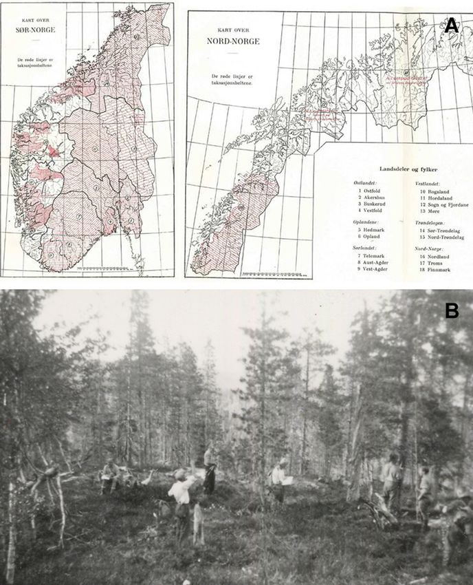
Fig. 1. Forest resources according to the latest SoEF report of Forest Europe (2020): A) Forest area in percent of country land area; B) Average growing stock per
hectare of forest available for wood supply.
3
T. Gschwantner et al. Forest Ecology and Management 505 (2022) 119868
Fig. 2. Early forest maps and management plans from Slovenia, Lithuania and Portugal: A) Trnovo forest 1769: Sub-units are numerated by the year of planned
harvest (Source: Perko et al., 2014/SFI); B) Kliošių Royal Forest administrative unit from 1790: Land use categories, tree species and age classes are marked by
different colours and signs (Source: Deltuvas, 2019/VMUAA); C) Machada e valle de Zebro: Compartments and stands are delineated and age-classes distinguished by
different colours (Source: Gomes, 1865/CEABN).
used and gradually perfected and stand estimates were aggregated for history of cartography (Harley and Woodward, 1987) and the manifold
groups of stands or higher-level management units. The production shift purposes of maps including orientation, exploration and exploitation of
from fuel wood to timber during the industrialisation (Appendix A) resources, state administration and taxation, warfare, or self-
required information about single trees and led to the development and representation of a state’s wealth. Also, the earliest large-area forest
continuous improvement of measurement techniques. Sample plots were representations for state territories in Europe are cartographic works or
recognised already in the early 18th century as cost-efficient alternative registers of forest lands that reach back to the early modern era. Most
to full tree census (Schwappach, 1886) and were at least occasionally examples feature forest area mapping and more or less detailed de
used to obtain GS estimates for stands (Prodan, 1965). The Central Eu scriptions of forests, but we can also recognise characteristics of modern
ropean stand-wise approach influenced the survey methods in many multi-source NFIs such as regular reporting and integration of various
countries. For instance, in Slovakia and Lithuania the first stand-level information sources (Table 1). In Sweden for instance, local governors
surveys started in the late 18th or early 19th century (Brukas et al., had to report on the forest situation in their counties from 1740 onwards
2002; Szarka and Bavlšík, 2011; Deltuvas, 2019) and the oldest local to the central administration (Anonymous, 1914). Wessely (1853) in
forest management plans in Serbia, Romania and Portugal (Fig. 2C) date Austria and similarly von Berg (1859) in Finland based their forest sta
back to the mid or second half of the 19th century (Stinghe and Sburlan, tistics on various information sources including travel observations, own
1941; Rego, 2001; Medarević, 2006). In the early 20th century stand- work experience, published material, and personal communication. The
wise surveys were also performed on larger areas in several countries, first attempt of country-level GS estimation from Sweden is reported for
e.g. in Estonia (Etverk, 1998), the state forests of Finland (Koivuniemi the year 1840 and was conducted by A.I. af Ström. Subsequent assess
and Korhonen, 2006), Latvia (Vasilevskis, 2007), Lithuania (Kuliešis ments followed in 1882 by J.O. Zellén and in 1905 by U. Wallmo (Anon
et al., 2010b), and Romania (Stinghe and Sburlan, 1941). Country-wide ymous, 1914). But, large-area estimation of GS remained methodically
forest management planning after World War II furthered the large-area challenging and led particularly in Northern Europe to the search for new
implementation of stand-wise inventories in many East-European coun approaches, while in other countries forest mapping, census or stand-
tries (Tomppo et al., 2010a) and the compilation-method to obtain wise approaches remained prevalent (e.g. Milizia Nazionale Forestale,
country-level results of GS (Loetsch and Haller, 1964). 1936; Lietuvos miškų statistika, 1939; BMLF and FBVA, 1960).
2.3. Towards large-area forest information 2.4. Sample-based NFIs
The desire for large-area information is most clearly manifested in the In the Northern European countries, vast and widely unsurveyed
4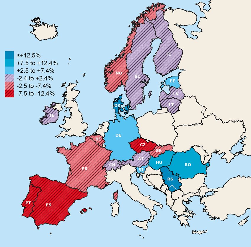
T. Gschwantner et al. Forest Ecology and Management 505 (2022) 119868
Table 1
Examples of historical large-area forest resource information until the early 20th century.
Year Description Reference
1517 Descripción y cosmografía de España by H. Colón, a collection of catastral information together with woodland and terrain Colón (1988)
description along the itinary to prepare a cartography of Spain.
1559 Register of woodlands and passages of game animals on the lands of Grand Dukedom of Lithuania. Volovič (1559)
1655 – 1659 Mapping of Ireland following the Cromwellian conquest, assessment of townlands and their value, including woodlands Simington (1953)
and boundaries of properties.
1737–1746 Mapping and description of Norway’s forests by the brothers J.G. and F.P. von Langen. Fryjordet (1992)
~1740 Reporting of local governors in Sweden on the forest situation in their counties to the central administration. Anonymous (1914)
1772 Land survey and forest area statistics on the territory of nowadays Latvia. Vasilevskis (2007)
1770–1778 Mapping of the Austrian Netherlands and the Prince-Bishopric of Liège in actual Belgium. Lemoine-Isabeau (1984), De Coene
et al. (2012)
1780–1820 Landscape survey in Denmark and mapping of forest area. Bradshaw (2004)
1805 Countrywide census and maps of wood for ship building in the French forests. Brenac (1984)
1817–1861 Franziszeischer Kataster of the Habsburg Empire, a complete estate cadastre with distinction of forest land, based on the Fuhrmann (2007), Stockmann (2016)
earlier land register Josefinisches Lagebuch (1786–1788).
1840 First estimation of GS, increment and timber consumption for entire Sweden and subsequent assessments of Swedish forest Anonymous (1914)
recources in 1882 and in 1905.
1853 Compilation of forest statistics for the Austrian alpine crown lands including forest area, average stand volume and growth. Wessely (1853)
1858 Report on the forest resources of Finland including a rough map on the condition of forest resources. von Berg (1859)
1867 First reliable land use area assessment including forests in Portugal. Ribeiro and Delgado (1868)
1874 Statistical yearbook founded by the Austrian Ministry of Agriculture containing agricultural and forest statistics. Braun (1974)
1878 First forest census on forest area based on combinations of official statistics covering the entire area of the German Empire, Schmitz et al. (2006)
periodically repeated and developed further, with most detailed information provided in 1937 including ownership, forest
types, condition and yield.
1881 Forest census and compilation of national statistics on forest area and tree species distribution in Denmark. Bastrup-Birk et al. (2010)
1878–1889 Survey of mainly public forests in France and preparation of 85 forest maps based upon the existing military maps. Brenac (1984)
1887 – 1902 Assessments for producing the Carta Agrícola e Florestal of Portugal. Basto (1936)
1907 First official statistics in Norway on forest area obtained by the Census of Agriculture. Det Statistiske Centralbyraa (1910),
Fryjordet (1962)
1912 First complete forest statistics in France containing forest area at canton level by property, tree species and silvicultural Daubrée (1912)
management.
forests and sparse road networks (e.g. Michelsen, 1995) required an measurements for GS estimation. However, it was not before the 1960s
alternative approach to the stand-wise surveys in Central Europe and that further countries also introduced sample-based NFIs (Fig. 4).
spurred the idea of using representative samples in large-area forest Additional countries followed in the 1980s and 1990s and in the two
inventories. The first line-sampling survey was made by A.I. af Ström in recent decades most countries in Europe had established sample-based
the 1840s in the Swedish province of Norrland (Loetsch and Haller, NFIs to obtain the required periodical information about the state and
1964; Zöhrer, 1980). This technique was used in Finland first in 1885, change of forest resources, efficiently and representatively, and ac
and in 1911–1912 in the municipalities of Sahalahti and Kuhmalahti cording to reliable statistical principles (Fisher, 1950). The introduction
(Ilvessalo, 1923). In 1907–1909, an inventory was conducted in the of regularly re-measured permanent sample plots facilitated the obser
municipality of Åmot in Norway, where sample plots and sample strips vation of change components, i.e. fellings, natural losses, surviving
were used (Vevstad, 1994). A trial inventory was undertaken in trees, and new trees (Kuliešis et al., 2016; Tomter et al., 2016). First
1910–1911 in Värmland to develop the methods for a country-wide NFI implemented in the 1980s by Austria, Switzerland, Sweden, Germany,
in Sweden. For the inventory of the vast state-owned coniferous forests Norway and Spain, today most NFIs rely on permanent plots or on a
located predominantly in northern Norway, a line sampling design was combination of permanent and temporary plots (Sections 4.1 and 4.2).
used as of 1914 (Breidenbach et al., 2020a). As the first country in the
world, Norway commenced a sample-based NFI by counties in 1919 and 3. Terminology and definitions
the first report was published for the county Østfold in the following
year (Landsskogtakseringen, 1920). Further county-reports were 3.1. Establishment of the term growing stock
released yearly until the completion of the first NFI in 1930 (Land
sskogtakseringen, 1933). The first Finnish NFI started in 1921, was The term growing stock originates from the Anglophone countries and
completed in 1924 and preliminary results were published the same year in regard to forestry describes the amount of wood volume stored by the
(Ilvessalo, 1924). Sweden’s first NFI began in 1923 and was completed trees on a certain forest area. Evelyn (1760) in his influential work Sylva
in 1929 (Fridman et al., 2014). The GS assessments of the first NFIs were used the term stock of timber already in this sense. Towards the early
carried out by measuring trees on parallel belts (Fig. 3) at a particular 20th century, the term growing stock apparently became more widely
compass bearing across the country (Axelsson et al., 2010; Tomter et al., used, for example through the forest mensuration textbooks by Schenck
2010; Breidenbach et al., 2020a), or by visual assessment of the stands (1905) and Graves (1906) and the forest terminology by the Society of
intersecting with parallel survey lines in combination with plot mea American Foresters (1916). Alternatively, in the earliest reports on
surements to calibrate and correct the visual estimates (Ilvessalo, 1927). world forest resources by Zon (1910) and Zon and Sparhawk (1923) this
Traversing the country on parallel belts or lines also served the purpose statistical quantity is denoted as present stand or stand of timber. The first
of mapping land uses, timber distribution, forest types, and topography world forest resources survey by the FAO (1948) used the term volume of
(Kangas and Maltamo, 2006). growing stock and argued the great diversity in the statistics available
In the 1950s, the road networks and transportation infrastructure from countries. Recommendations for standardising the use of symbols
had been extended in the Northern European countries. Belt and line and abbreviations of terms in forest mensuration were made by IUFRO
sampling became less efficient and sampling designs changed towards (1959), and Päivinen et al. (1994) developed guidelines for the
cluster plots (Fridman et al., 2014; Korhonen, 2016; Tomter, 2016; compatible collection and reporting of forest monitoring data. The first
Breidenbach et al., 2020a). The subsequently emerging NFIs in Europe homogeneous set of terms and definitions was achieved in the global
were based on single or cluster plots to obtain the sample tree Forest Resources Assessment FRA 2000 and its contribution on
5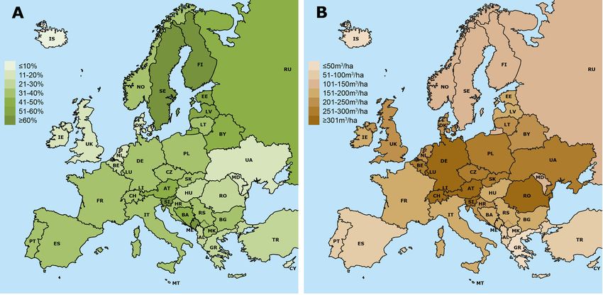
T. Gschwantner et al. Forest Ecology and Management 505 (2022) 119868
Fig. 3. The early NFIs in Norway and Sweden: A) Coverage and density of sampling strips in Southern and Northern Norway; numbers indicate counties as delineated
inventory areas, parallel red lines are the inventory strips (Source: Landsskogtakseringen, 1933/NIBIO); B) Field work of the Swedish NFI in 1939 (© SLU).
temperate and boreal forests TBFRA (FAO, 1998; UNECE/FAO, 2000; masa (Latvian), Medyno tūris (Lithuanian), Stående volum (Norwegian),
FAO, 2001). In the subsequent FRAs the GS definition was revised (FAO Volume em crescimento (Portuguese), Volumul de lemn pe picior (Roma
2004, 2010, 2012, 2018) and also other international reporting pro nian), Зaпac дpeвocт oя (transcribed Zapas drevostoja, Russian), Dubeća
grammes included GS in their glossaries (IPCC, 2003, 2006; Forest drvna zapremina (Serbian), Zásoba dreva (Slovak), Lesna zaloga (Slove
Europe, 2015). Other sources of GS definitions are forestry dictionaries nian), Volumen en pie (Spanish), Virkesförråd (Swedish). These terms are
and similar collections (e.g. Helms, 1998; Delijska and Manoilov, 2004; defined in European NFIs by similarly composed definitions that specify
IUFRO, 2021). the minimum dbh, the tree parts included, and the living and standing
status of perennial woody plants taken into account in GS estimation
3.2. Terms and definitions for growing stock in European NFIs (Vidal et al., 2008). However, national definitions reflect the specific
historical development and information needs and hence vary between
In other European languages comparable terms for growing stock are countries. For example, the dbh-thresholds range between 0 and 12 cm
Zásoba dříví (Czech), Stående vedmasse (Danish), Kasvava metsa tagavara and also the included tree parts indicate considerable variation (Fig. 5)
(Estonian), Puuston tilavuus (Finnish), Matériel sur pied (French), Ste as well as the associated thresholds for stump height, top diameter and
hender Holzvorrat (German), ξυλαπ όθεμα (transcribed ksilapothema, branch diameter (Gschwantner et al., 2019). A unified GS definition was
Greek), Élöfakészlet (Hungarian), Provvigione legnosa (Italian), Krāja or established by the European NFIs for the purpose of harmonised
6
T. Gschwantner et al. Forest Ecology and Management 505 (2022) 119868
Fig. 4. Sample-based NFIs in 23 European countries over time. Remark: The inventories in France were conducted at Département-level from 1960 to 2004, resulting
in overlapping NFI cycles. Abbreviations: WAL Wallonia, VLG Flanders, GDR German Democratic Republic, FRG Federal Republic of Germany.
international reporting (Section 5). in the area (Mandallaz, 2008). Sample plots located on forest land are
determined by a forest definition and associated thresholds for mini
4. Current methods of European NFIs mum crown cover, area, width, and potential or actual tree height
(Schreuder et al., 1993; Köhl et al., 2006; Vidal et al., 2008; Lanz et al.,
4.1. Overall sampling schemes 2019b). The sample plots have a specific arrangement, shape and size
and defined sample tree inclusion probabilities (Section 4.3). Fig. 6 gives
For monitoring the status and development of GS, European coun an overview on sampling designs of European NFIs. Note, however, that
tries have implemented national sampling frames. A sampling frame is particular regions within countries may deviate from the general
defined by the area from which the sample elements are selected. The scheme. Large-area NFI campaigns are either continuously or periodi
sample elements are a number of sample plots. In the infinite population cally conducted. In continuous NFIs, the sampling frame is systemati
approach the population is the infinite number of potential sample plots cally divided into disjoint panels (e.g. Roesch, 2007), where an
Fig. 5. Tree parts taken into account in the growing stock definitions of European NFIs, illustrated by the respective colors. Remarks: aConifers; bBroadleaves; cOther
oaks and other broadleaves; dAcacia sp., Castanea sativa, Eucalyptus globulus, Pinus pinaster, Pinus pinea, other conifers; eQuercus suber; fQuercus rotundifolia.
7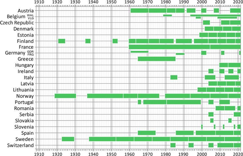
T. Gschwantner et al. Forest Ecology and Management 505 (2022) 119868
individual panel is a set of samples that are measured on one and the NFIs offset the cluster position from the grid intersection point and the plot
same occasion (e.g. year). Individual panels cover either the whole location from the cluster corners (e.g. Jansons and Licite, 2010; Kuliešis
country by interpenetrating panels (e.g. Kuliešis et al., 2010a; Lanz et al., 2010a). Permanent plots and temporary plots are usually arranged in
et al., 2019b; Breidenbach et al., 2020a) or certain counties by regional separate grids. Semi-temporary plots denote plots that are re-measured
panels (e.g. Alberdi Asensio et al., 2010). Periodic NFIs often complete only once (Hervé, 2016), or at large time intervals (Rondeux et al., 2010).
the field inventory within one or a few years and cover the whole
country by a single panel (ICNF, 2016; DAFM, 2018; Kleinn et al., 2020). 4.3. Sample plot features
Once all sample plots are measured, the procedure reinitiates in the
subsequent year in continuous inventories or after a break of up to ten Sample plots are the basic unit for comprehensive terrestrial mea
years in periodic inventories. The sampling density is either uniform surements and the ground reference for remotely sensed data (Section
over the whole country, or varies according to regional stratification of 4.9). The plot configuration describes the size, shape, and components of
the forest area. A remote-sensing-based assessment previous to the field plots serving as sampling units for various tree–, stand- and site-specific
inventory pre-classifies sample plots into forest, potential forest, and variables (Vidal et al., 2016a). Also line-intersect samples for e.g. lying
non-forest, while other inventories conduct the forest-non-forest deci dead wood are occassionally attached to the plots (e.g. Kučera, 2016;
sion terrestrially during the field assessment. Two- or more-phase sam Breidenbach et al., 2020a). Maps and registers often provide informa
pling utilises a higher sampling density in the first phase remote sensing tion on administrative regions, ownership categories, ecoregions, land
interpretation previous to the terrestrial inventory (Mandallaz, 2008; use, forest management or forest types and are attributed either to the
Lanz et al., 2019b; Gasparini and Di Cosmo, 2016; Grafström et al., plot centre or to sub-divisions of the sample plot area. For GS moni
2017). Sample plots are either single sampling locations or clusters. toring, European NFIs use either plots consisting of one circle to include
Permanent sample plots are invisibly marked for refinding and polar and measure all trees above a certain dbh-threshold (Tomé et al., 2016;
coordinates of sample trees are recorded, while temporary plots are used Tomter, 2016), or concentric circular plots with fixed radii that consist
and visited only once. NFI sampling designs involve cost-benefit con of two (e.g. Kušar et al., 2010; Bosela and Seben, 2016; Gasparini and Di
siderations and optimisation that aim on a reasonable relation between Cosmo, 2016; Lanz et al., 2016; Marin et al., 2016), three (e.g. Kuliešis
resources spent in terms of e.g. travel costs, personnel costs and work et al., 2003; Alderweireld et al., 2016; Hervé, 2016; Kolozs and Solti,
flow organisation on the one hand and the amount and quality of 2016; Nord-Larsen and Johannsen, 2016; Pantic et al., 2016; DAFM,
measurements and yielded information on the other hand (e.g. Patterson 2018), or four circles (e.g. Alberdi et al., 2016a) arranged at a common
and Reams, 2005). center point. The concentric circles refer to different dbh-thresholds, the
inner circle having the lowest and the outer the highest dbh-threshold
4.2. Systematic sampling approaches (Fig. 7). Angle-count sampling according to Bitterlich (1948) is still
applied by two NFIs (Gschwantner et al., 2016; Riedel et al., 2016,
NFI sampling schemes accommodate country-specific conditions Kleinn et al., 2020), with a maximum circle size limit recently intro
(McRoberts et al., 2012a) and most commonly rely on systematic sam duced by the Austrian NFI (Berger et al., 2020). Many European NFIs
pling. Terrestrial sampling is based on regular grids (Lawrence et al. 2010) have lately introduced additional small and mostly circular off-centre
and grid sizes range between 1.0 km × 0.5 km and 5.0 km × 5.0 km. In the plots for trees below the dbh-threshold to improve the data basis
less productive regions of Northern European countries, grid sizes up to about regeneration trees and to support international harmonisation.
20.0 km × 20.0 km are used (Table 2). Different sampling densities within The number, size and dbh-thresholds of concentric circles and
a country relate to spatial differences in forest conditions, i.e. percentage of similarly the basal area factor of angle-count sampling is chosen
forest land, forest productivity, and road networks (e.g. Axelsson et al., depending on the dbh-distribution in a country, the number of sample
2010; Robert et al., 2010; Tomter et al., 2010; Marin et al., 2016; Bouriaud trees to be measured, the workflow of assessments at the plot locations,
et al., 2020). The grid intersection points are either the center points of and the envisaged coefficient of variation between sample plots (Loetsch
single plots, or the corner or center points of cluster plots. In restricted et al., 1973). Compared to other plot layouts, circular plots are efficient
random sampling, the location of usually single plots is randomly selected under European forest conditions, they are relatively easy to establish,
in an area of determined size and shape established at the grid intersection can be efficiently marked with a single mark at the plot centre, and
points (e.g. O’Donovan and Redmond, 2010), or, in tessellated sampling enable the best visibility over the plot from the central point. The pe
designs within the grid-cells (e.g. Gasparini et al., 2013; Hervé, 2016; riphery zone of the plot is the smallest possible relative to the plot area
Kučera, 2016). NFIs that use cluster plots rely often on square-shaped and minimizes the number of borderline trees that require exact distance
clusters with side-lengths ranging between 150 and 1800 m. Alternative measurement.
cluster shapes are L- and open rectangular shapes (Korhonen, 2016). Some
Fig. 6. Sampling schemes by number of European NFIs. Remarks: a One NFI changes since 2020 towards continuous inventory (SI); b Three NFIs use two- or more-
phase sampling (CH, IT, SE); c Six NFIs use combined permanent and temporary plots (BE, DK, EE, FI, RO, SE); d One NFI re-measures plots once, denoted as semi-
temporary plots (FR).
8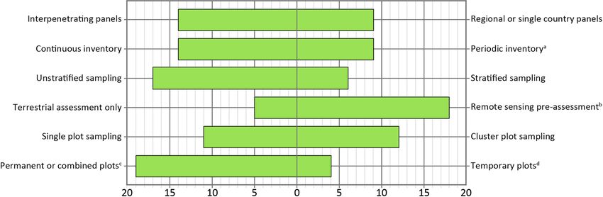
T. Gschwantner et al. Forest Ecology and Management 505 (2022) 119868
4.4. Sample tree measurements
Features of terrestrial NFI sampling used for growing stock monitoring. Remarks: a GR: random plot selection; b NO: temporary plots for periodically conducted county-level inventories; c SI: since 2020 change towards
Concentric circular plots, Rectangular plot
Concentric circular plots, Rectangular plot
The measurement and assessment of sample tree variables such as
Angle count sampling, Circular plot
tree species, dbh, tree height, and upper diameter (Tomppo et al., 2010a;
Vidal et al., 2016a) provide the input data for single-tree volume models
(Section 4.6). Tree-shape categories may be also required (e.g. Alberdi
Concentric circular plots
Concentric circular plots
Concentric circular plots
Concentric circular plots
Concentric circular plots
Concentric circular plots
Concentric circular plots
Concentric circular plots
Concentric circular plots
Concentric circular plots
Concentric circular plots
Concentric circular plots
Concentric circular plots
Concentric circular plots
Concentric circular plots
Concentric circular plots
et al., 2016a). The dbh is the most cost-efficiently and precisely
Angle count sampling
Angle count sampling
measurable tree variable (Spurr, 1952), while other measurements are
Single circular plot
Single circular plot
more time-consuming, associated with larger uncertainties (Berger
Configuration
et al., 2014), and therefore measured only on a subset of sample trees
(Section 4.5). Some NFIs measure the circumference at breast height
instead of dbh (e.g. Alderweireld et al., 2016; Hervé, 2016). Classical
callipers and measuring tapes are in frequent use (Table 3). Large
diameter trees above the calliper scale length require diameter mea
surement with a tape (e.g. Düggelin et al., 2020). Electronic diameter
measurement devices feature automatic reading, data storage and
Permanent and semi-temporary
wireless data transmission to the field computer. The efficiency of height
Permanent and temporary
Permanent and temporary
Permanent and temporary
Permanent and temporary
Permanent and temporary
Permanent and temporary
measurements has increased through the use of ultrasonic distance
measurement, especially in dense stands. Crown length is obtained as
difference between the tree height and height to the crown base. Upper
Semi-temporary
Plot features
diameters are measured either at a fixed height of e.g. seven meters with
Temporary
Temporary
Temporary
Permanent
Permanent
Permanent
Permanent
Permanent
Permanent
Permanent
Permanent
Permanent
Permanent
Permanent
Permanent
a pole calliper (Lanz et al., 2016), at relative heights of e.g. 30 % tree
height with indirect methods (Gschwantner et al., 2016; Riedel et al.,
Type
2016), or at the height corresponding to e.g. 10 % of bole diameter
decrease (Morneau, 2015). New instruments like Terrestrial LiDAR
sensors may become used in future large-area field inventories (Bauwens
et al., 2016; Ghimire et al., 2017).
Plot number
5 to 14
4 to 12
4.5. Methods of sub-sampling
4 to 8
10
4
1
1
4
8
1
4
4
1
1
4
1
1
4
4
1
1
1
1
Many NFIs take a smaller sub-sample for time-consuming height and
upper diameter measurements within the larger sample of dbh-
measured trees, also denoted as two-stage sampling (Mandallaz, 2008;
Side-length (m)
Mandallaz and Massey, 2012). Four methodical groups regarding sub-
1200 – 1800
300 – 1800
sampling can be identified among European NFIs. A basic distinction
250 – 500
20 – 40
can be drawn between NFIs that take the measurements on all sample
200
200
800
150
200
250
250
200
trees (Method 1), from NFIs that use a sub-sample (Methods 2 – 4)
–
–
–
–
–
–
–
–
–
–
–
(Fig. 8). Method 2 refers to NFIs that use two sets of volume models, one
set of more precise volume models for the smaller sub-sample and using
Cluster features
e.g. dbh, height and upper diameter as predictors, and a second set of
L- and [-shape
tariff functions (e.g. Herold et al., 2019; Breidenbach et al., 2020a) or
Hexagonal
Quadratic
Quadratic
Quadratic
Quadratic
Quadratic
Quadratic
Quadratic
Quadratic
Quadratic
Quadratic
non-parametric functions (e.g. Korhonen and Kangas, 1997) that are
Shape
parameterised with the sub-sample volumes and applied to calculate the
continuous inventory with 2.0 km × 2.0 km grid and interpenetrating panels.
volumes of the trees in the larger sample. Method 3 uses the sub-sample
–
–
–
–
–
–
–
–
–
–
–
tree measurements to parameterise data-models such as height curves
Plot arrangement
(e.g. Sloboda et al., 1993; Ozolins, 2002; Kuliešis et al., 2014) or upper
diameter models (e.g. Korhonen, 1992; Sloboda et al., 1993; Gabler and
Single plots
Single plots
Single plots
Single plots
Single plots
Single plots
Single plots
Single plots
Single plots
Single plots
Single plots
Clustering
Schadauer, 2008), which are used to predict the missing heights or
Cluster
Cluster
Cluster
Cluster
Cluster
Cluster
Cluster
Cluster
Cluster
Cluster
Cluster
Cluster
upper diameters of not measured sample trees. The predicted data enter
the volume models as input variables. Method 4 uses the sub-sample tree
measurements to derive stand-specific variables like dominant height or
mean height required as explanatory variables in volume models (e.g.
3.0 to 20.0 × 20.0
to 20.0 × 20.0
Tomé et al., 2007b; Dagnelie et al., 2013). Stand variables can also be
and 4.0 × 4.0
2.0 to 4.0 × 4.0
to 9.0 × 9.0
(2.0 × 2.0)
used as explanatory variables in height curves (Bastrup-Birk et al., 2010;
Kuliešis et al., 2014; Gasparini and Di Cosmo, 2016) or tariff functions
(Herold et al., 2019) and constitute hybrids of Methods 2 and 4 or 3 and
(km £ km)
Grid size
3.9
0.5
2.0
2.0
5.0
1.0
4.0
2.0
1.0
4.0
4.0
3.0
2.0
2.0
4.0
4.0
4.0
1.0
3.0
1.4
4.
3.9 ×
1.0 ×
2.0 ×
2.0 ×
5.0 ×
3.0 ×
1.0 ×
2.0 ×
4.0 ×
2.0 ×
1.0 ×
4.0 ×
4.0 ×
3.0 ×
2.0 ×
2.0 ×
4.0 ×
4.0 ×
4.0 ×
1.0 ×
3.0 ×
1.4 ×
The sub-sample trees are either a systematic or randomised choice
per sample plot. Conditional inclusion probabilities aim at optimising
–
the sub-sample by e.g. including sub-sample trees proportional to model
residuals and to a targeted number of re-measured sub-sample trees
(Lanz et al., 2019b). Due to harvests, the number of sub-sample trees
Czech Republic
NFI – Country
cannot be exactly predicted prior to field measurements, however, a
Switzerland
Slovenia c
Lithuania
Norway b
Denmark
Germany
Romania
Hungary
Portugal
Slovakia
sufficient number of measurements is required for the species, dbh-
Greece a
Belgium
Sweden
Finland
Estonia
Austria
Ireland
Table 2
France
Serbia
Latvia
Spain
classes and stand layers represented in the sample. The size of sub-
Italy
samples is usually between 10 and 35 % of dbh-measured sample
9
T. Gschwantner et al. Forest Ecology and Management 505 (2022) 119868
Fig. 7. Examples of plot configurations used for growing stock monitoring, harmonised presentation: A) Germany - Angle-count sampling and concentric regen
eration plots; B) Latvia and Lithuania – two concentric circles, with one quarter of the inner circle serving as third tree sampling unit, and rectangular regeneration
plot; C) Romania – two concentric circles and two regeneration plots; D) Spain – four concentric circles and inner circle serving as regeneration plot.
trees. Common inclusion procedures are every 6th or 7th sample tree, obtained from the two to five largest trees, or from the central dbh-class.
every 10 m2 or 15 m2 of represented basal area per hectare, angle-count Some NFIs measure also trees outside the plot in the surrounding stand
sampling with large basal area factors of e.g. 12 m2/ha or basal area to derive stand variables.
factors depending on the stem number, or a randomised choice of e.g. 6
trees per plot. Stand variables like dominant height or mean height are
Table 3
Sample tree measurements and instruments used for growing stock monitoring by number of NFIs. Remarks: a Ten NFIs use the measuring tape only for large-diameter trees; b
References: Bitterlich (1992), Laser Technology (2006), Haglöf Sweden (2014-2017), IFER (2020).
Variable Classical calliper Electronic calliper Measuring tape a Pole calliper Relascope® b
Criterion® b
Vertex® b Field-map® system b
Dbh 14 4 13
Girth 2
Upper diameter 1 2 1 2
Tree height 1 18 4
Height to crown base 2
10T. Gschwantner et al. Forest Ecology and Management 505 (2022) 119868
Fig. 8. The use of sub-sampling by European NFIs. Tree height: Method 1 - AT, BE (broadleaved stands), GR, RO, RS, ES; Method 2 - FI, NO, SE, CH, FR; Method 3 -
CZ, DK, EE, DE, HU, IE, IT, LT, LV, PT, SK, SI (since 2020); Upper diameter: Method 2 – CH; Method 3 - AT, DE; Dominant height: Method 4 - BE (conifer stands), IT,
PT; Mean height: Method 4 - DK, SI.
4.6. Volume models Kenstavičius, 1976; Sopp and Kolozs, 2000). As the tree shape may
change over time, recurrent tree measurements can be used to evaluate
4.6.1. Development of volume models the validity of volume models (e.g. Kušar et al., 2013; Herold et al.,
Country- and tree species-specific single-tree volume models are 2019) or to parameterise up-dated models (e.g. ICONA, 1990; Morneau,
implemented by European NFIs to estimate the sample tree volumes 2015; Kangas et al., 2020). Other NFIs update the height-curves and
based on the previously described measurements. Volume models are upper-diameter models for each inventory (e.g. Gabler and Schadauer,
developed and parameterised using large data sets of thousands to ten- 2008), or take into account the current local diameter-height relation
thousands of measured trees, representing the forest conditions or ship (e.g. Tomter et al., 2010; DAFM, 2018).
relevant regions within a country, and obtained in customised and
laborious measurement campaigns. The measurements have been 4.6.2. Volume model types
gathered at harvesting sites or research plot networks following detailed Single-tree volume models can be grouped by the modelling concept,
measurement instructions (e.g. Grundner and Schwappach, 1922; Pet the function type and the required input variables. Taper curves, form
tersson, 1955; Vestjordet, 1967; Braun, 1969; Näslund, 1971; Madsen, factor functions, and volume functions are applied by European NFIs
1987; Petráš and Pajtík, 1991; Kaufmann, 2001), or on standing trees on (Table 4). Frequently, more than one set of volume models is imple
NFI plots (e.g. Laasasenaho, 1976, 1982; Morneau 2015). The recorded mented, to obtain different target volumes of over-bark or under-bark
data include section-wise stem diameter measurements, tree species, stem volume (e.g. Braastad, 1966; Brantseg, 1967; Vestjordet, 1967;
dbh, height, upper diameters, crown length, stand and site variables, Petráš and Pajtík, 1991; Bauger, 1995; Paulo and Tomé, 2006; Tsitsoni,
and essentially have to cover the existing range of dendrometric attri 2016), to include or exclude the branch volume of broadleaves (e.g.
butes (Köhl et al., 2006). The volume of stem sections is obtained by the Petráš and Pajtík, 1991), to allow different top-diameter limits (Madsen,
formulae of Huber (1828), Smalian (1837), or the frustum of a cone and 1987), or to estimate the assortments of standing stems (Laasasenaho,
summed up for the whole tree. Volume tables were constructed from the 1976, 1982; Rohner et al., 2019). The function types of volume models
measurements until the first half of the 20th century, and later in some include power and exponential functions as well as linear combinations
cases served as data basis for the parametrisation of volume functions of usually transformed variables. To capture the variation in stem forms
and adaptation to country-level conditions (e.g. Čokl, 1957; Kuliešis and across the country, the volume models require either upper diameters as
Table 4
Modelling concepts of single-tree volume models used by European NFIs for growing stock estimation.
Modelling Description Country - NFI
concept
Taper curve Taper curves describe the stem shape along the stem axis from the base point up to the stem tip and predict the stem DE, DK, FI, IE
diameter at a specified height, or the height for a specified diameter. The integral of stem taper curves produces the
stem volume and defined stem segments.
Form factor Form factor functions describe the relationship between the tree volume and the reference cylinder volume having a AT, LT, CZ, EE, FR
function cross-sectional area equal to the basal area at a defined height (e.g. breast height) and a height equal to the stem
length.
Volume function Volume functions directly describe the tree volume depending on a set of explanatory variables. BE, CH, DK, ES, FI, GR, HU, IT, LV, NO,
PT, RO, RS, SE, SI, SK
11T. Gschwantner et al. Forest Ecology and Management 505 (2022) 119868
input variables (e.g. Braun, 1969; Laasasenaho 1976, 1982; Kublin, unbiased model-based variance estimators. Post-stratification is applied
2003), or stand and site variables (e.g. Čokl, 1957; Dagnelie et al., 2013; to maintain the additivity of regional estimates with country-level es
Herold et al., 2019), or regional volume models for different tree shapes timates (e.g. Lanz et al., 2019b) or to construct less variable groups of
are parametrised (e.g. ICONA, 1990). A compilation of form factor and plots for age classes, growth stages or species composition (Moravcik
volume functions applied by European NFIs is given in Appendix B. For et al., 2010). Weights are also applied for the combination of permanent
taper curve models please refer to Laasasenaho (1982), Madsen (1985), and temporary plot estimates (Axelsson et al., 2010) or for the combi
Riemer et al. (1995) and Kublin (2003, 2013). The predicted tree vol nation of the individual years into an multiannual NFI cycle estimate
umes differ among NFIs in terms of included tree parts as specified by (Adermann, 2010). Further details on forest inventory estimators are
the national GS definitions (Section 3.2). available from the textbooks of Schreuder et al. (1993), Gregoire and
Valentine (2007), and Mandallaz (2008).
4.7. Expansion to larger areas
4.7.2. Uncertainty components
4.7.1. Growing stock estimators Sampling error is estimated as the variation between the sampling
The sample of trees measured at the sample plots are required to units (Formula 3) and originates from measuring only a sample of plots.
estimate the parameters of the population and the uncertainty of the Cunia (1965) identified volume model error and measurement errors as
estimates. In terms of GS, the population parameters are typically the additional uncertainty sources, and similarly Gertner and Köhl (1992)
mean volume per unit of area and the totals for countries or other devided non-sampling errors into function error, measurement error and
defined geographic areas. An estimator denotes the calculation rule by classification error. The function error is due to the use of volume
which an estimate i.e. the value of a population parameter is obtained models to predict the individual-tree volume (Section 4.6) and can be
from the sample. Design-based estimators are usually applied for large- attributed to model misspecification, uncertainty in the values of inde
area GS monitoring by European NFIs (Kangas and Maltamo, 2006; pendent variables, uncertainty in model parameter estimates, and re
Tomppo et al., 2010a) as they are unbiased for reasonably large samples. sidual variability around model predictions (McRoberts and Westfall,
Design-based estimators and their properties derive from the inclusion 2014). The models required to predict unmeasured input variables of
probabilities of sample trees (Mandallaz, 2008). The corresponding GS volume models (Section 4.5) are also a source of uncertainty (Westfall
of an individual NFI sample plot per hectare is equivalent to the sum of et al., 2016). The measurement error can be distinguished into instru
sample tree volumes multiplied by their respective representation factor mental error and operator error (Schreuder et al., 1993). The uncer
that is the inverse of their inclusion probability: tainty components influence the accuracy and precision of GS results,
mj
the first describes the systematic deviation (“bias”) from the true value,
∑
Vha,j = Vi,j ∙f i (1) while the second refers to the reproducibility under unchanged condi
i=1 tions (Cochran, 1977). Köhl (2001) found that sampling error makes by
far the highest contribution to the overall uncertainty and that bias may
where Vi,j is the volume of the ith tree on the jth sample plot, mj is the
occur as a result of model errors or measurement errors. Therefore, NFIs
total number of sample trees on the sample plot j, fi is the representation
have implemented comprehensive Quality Assurance and Quality Con
factor, and Vha,j is the GS per hectare of plot j. In the basic form under
trol (QA/QC) measures that include detailed field instructions, training
simple random sampling, the GS estimators of the arithmetic mean
of personnel, control surveys, testing of measurement instruments,
volume per hectare and the corresponding standard error SE for a given
evaluation and updating of models, and investigation of the influence of
stratum are:
measurement errors and model uncertainties on large-area volume es
∑n
̂ = j=1 Vha,j timates (e.g. Gasparini et al., 2009; Berger et al., 2012, 2014; Brei
V (2)
n denbach et al., 2014; McRoberts and Westfall, 2014; Traub et al., 2019).
and
√̅̅̅̅̅̅̅̅̅̅̅̅̅̅̅̅̅̅̅̅̅̅̅̅̅̅̅̅̅̅ 4.8. Wood quality and assortments
√∑
√n ( ̂ )2
√
√
Vha,j − V
1 The mere information about GS does not sufficiently address the
̂ ) = j=1
SE( V ∙√̅̅̅ (3) information needs on available wood resources and potential end-use.
n− 1 n
All European NFIs assess quality-related tree variables such as tree
where V
̂ is the mean volume per hectare, SE( V)̂ is the standard error species, diameter, curvature, branchiness, and damages (Bosela et al.,
of the mean, and n is the number of plots in the stratum. Total GS ( V
̂ total ) 2016). A direct classification of sample trees in stem quality classes is
in the stratum and its standard error are obtained by multiplication of conducted by about two thirds of European NFIs, but only one quarter
the mean volume per hectare with the stratum area A: uses the stem quality variables to estimate assortments (Bosela et al.,
2016). The assortment of standing stems usually relies on taper curve
̂ ∙A
̂ total = V
V (4) models (e.g. Laasasenaho, 1982; Kaufmann, 2001; Kublin, 2003) for the
distinction of stem segments according to length and diameter classes of
and timber trade guidelines, and on the field assessments of stem quality
traits (Eckmüllner et al., 2007; Rohner et al., 2019). Despite doubts in
̂ )∙A
̂ total ) = SE( V
SE( V (5)
the reliability of visual appraisals of external quality features (Bosela
In most cases, forest area (Aforest) will also be a quantity estimated et al., 2016), several studies demonstrated the potential for stem grading
from NFI data and the mean GS per unit of forest area is the ratio of the of standing trees (Eckmüllner et al., 2007; Rais et al., 2014; Power and
estimated total volume in forest and the estimated forest area (Man Havreljuk, 2016; Malinen et al., 2018). The assortment models by Petráš
dallaz, 2008). Variants of these basic estimators are implemented by and Nociar (1990, 1991a, 1991b), Mecko et al. (1993), and Petráš and
European NFIs and concern mainly the use of strata weights and spe Mecko (1995) are based on a large sample material collected across
cifics in the standard error calculation such as using cluster-level esti Slovakia and were applied in a case study using an independent data set
mates, or groups of clusters. Most NFIs deliberately use the above from Czech Republic (Vidal et al., 2016c). Nevertheless, a transnational
variance estimators although they are known to be conservative for application of stem quality models on larger areas is at present
systematic sampling, i.e. they overestimate the variance (Magnussen complicated by the existing differences in national timber trade regu
et al., 2020). The Finnish NFI by default takes the spatial correlation of lations and different wood quality-related assessments of NFIs (Bosela
sample plots into consideration (Matérn, 1960), which results in nearly et al., 2016; Power and Havreljuk, 2016).
12You can also read