FP18 / FP38 Atmospheric Trace Gases - Physikalisches ...
←
→
Page content transcription
If your browser does not render page correctly, please read the page content below
FP18 / FP38
Atmospheric Trace Gases

              Institute of Environmental Physics
                    University of Heidelberg
                            Germany

                Document Version: 04.01.2022

                  compiled by Christoph Kern
revised by Martin Horbanski, Tilman Hüneke, and Marvin Knapp
Safety Instructions
Before starting the experiment, students must be familiar with the laboratory regulations. A
printed version of the regulations can be found next to the laboratory entrance. In particular,
the following sources of hazard will be encountered during the course:

Nitrogen dioxide cuvette
For parts of the experiment a nitrogen dioxide (NO2 ) cuvette with an NO2 volume mixing
ratio between 0.5 and 1.0% will be used. NO2 is harmful by inhalation. In case of nausea or
respiratory tract irritation call a poison control center or doctor. In case of release of gas from
the cuvette immediately leave the room and open windows if possible. Inform your experiment
supervisor. Storage may only be carried out in well-ventilated areas. The cuvette must therefore
be returned to an appropriate room after completion of the experiment.

Ethanol solution
Occasionally ethanol solution has to be applied to clean the optics in the telescope. Inhalation,
eye and skin contact should be avoided. When working with it, wear protective gloves and eye
protection. Keep the container away from any source of ignition and keep it tightly closed,
if not in use. In case of contact with eyes, flush them with water for a few minutes. After
swallowing drink plenty of water, then seek medical advice immediately.

Ultra violet (UV) radiation
In this experiment, a UV light source is used. UV radiation irritates and damages the eyes.
Skin irritation and even severe burns can occur in case of continuous UV exposure. When
working with the lightsource wear appropriate protective goggles. Do not look directly into the
light. Avoid direct exposure of the skin. If possible, screen the optical setup. Do not use the
light source longer than necessary.

Details on the listed hazards can be found in the information sheets attached to the labo-
ratory regulations. By signing the ’Safety Briefing - Signature List’, you confirm, that you have
read and understood these instructions.

                                                 I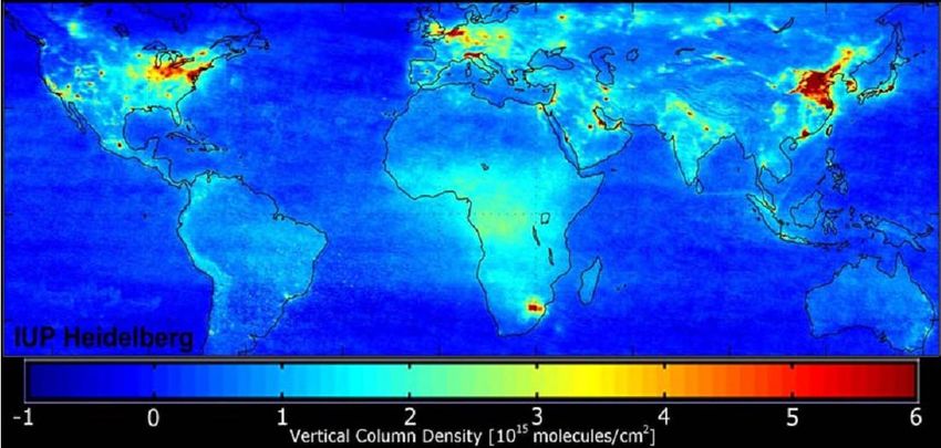
Introduction
Differential Optical Absorption Spectroscopy (DOAS) is a widely used technique for the detec-
tion of atmospheric trace gases in the atmosphere. It is based on the wavelength dependent
absorption of light by atmospheric constituents. Various trace gases can be identified simultane-
ously by their spectral signatures which act as an individual ’fingerprint’. The DOAS technique
has been implemented on several platforms: from ground, on aircrafts, balloons and satellites,
and by using either artificial light sources, scattered sunlight or direct sun- or moonlight.
Ground-based DOAS observations of scattered sunlight is very suitable both for long term mea-
surements of atmospheric constituents, and for measurements in the field using small portable
instruments. The latter can be used, for example, to study emissions from volcanic plumes or
the emission of reactive trace gases from remote salt lakes. Since those instruments are easy to
maintain, they are ideally suited for the operation in remote regions with restricted technical
infrastructure.
This experiment offers the opportunity to gain insight into spectroscopic remote sensing tech-
niques, which are widely used to study the composition of the Earth’s atmosphere. Differential
optical absorption spectroscopy has been developed by U. Platt and D. Perner at the Institute
of Environmental Physics of the University of Heidelberg. A relatively new application of this
measurement technique is Multi-Axis DOAS (MAX-DOAS), which has an enhanced sensitivity
for trace gases near the surface and allows to gain information on their vertical distribution.
The topics covered by this experiment are:
To gain insight in the chemistry of the troposphere and stratosphere, in particular re-
garding ozone and NO2
To become familiar with spectroscopy and spectroscopic analysis techniques
To gain insight into the radiative transfer in the Earth’s atmosphere
To learn how to determine a trace gas concentration with DOAS
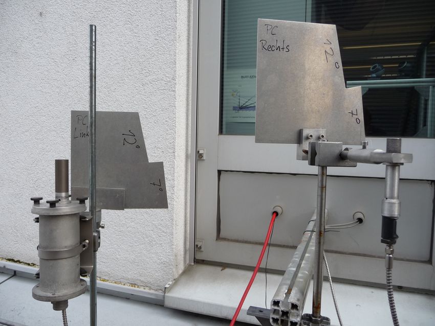
Instrumentation:
Passive DOAS instrument with spectrograph/detector unit
Quartz fiber
Temperature regulator
Halogen lamp
Mercury vapor lamp
Computer with measurement and analysis software
Glass cell filled with NO2
II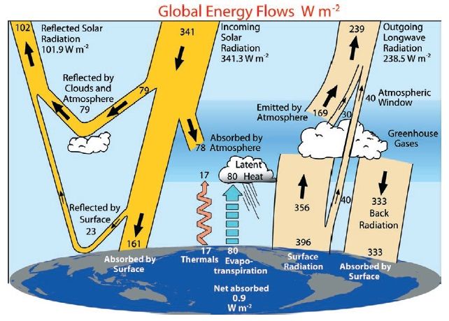
Study guide
Before starting the experiment, please take the time to review these materials. While you do
not need to know the exact step by step procedure of the experiment, you should be able to
answer the following questions:
How are ozone and nitrogen dioxide (NO2 ) distributed in the atmosphere? What are
typical concentrations of these species? How do the concentrations vary with the time of
day?
What is the importance of ozone in the stratosphere? What is the ozone hole? How is it
formed?
What is the importance of ozone and NO2 in the troposphere?
What is the Beer-Lambert law of absorption? What does it describe?
What does the word differential mean in Differential Optical Absorption Spectroscopy
(DOAS). Why is absolute absorption spectroscopy difficult to apply in the atmosphere?
What components contribute to a measured spectrum?
What equipment is necessary to record an atmospheric spectrum and why?
What is a slant column density (SCD)? What is a vertical column density (VCD)?
What knowledge is required in order to calculate trace gas concentrations from SCDs?
What is a Langley Plot? What is it used for?
What is Multi-Axis DOAS (MAX-DOAS)? How can information about the vertical profile
of a trace gas species be obtained with this technique?
III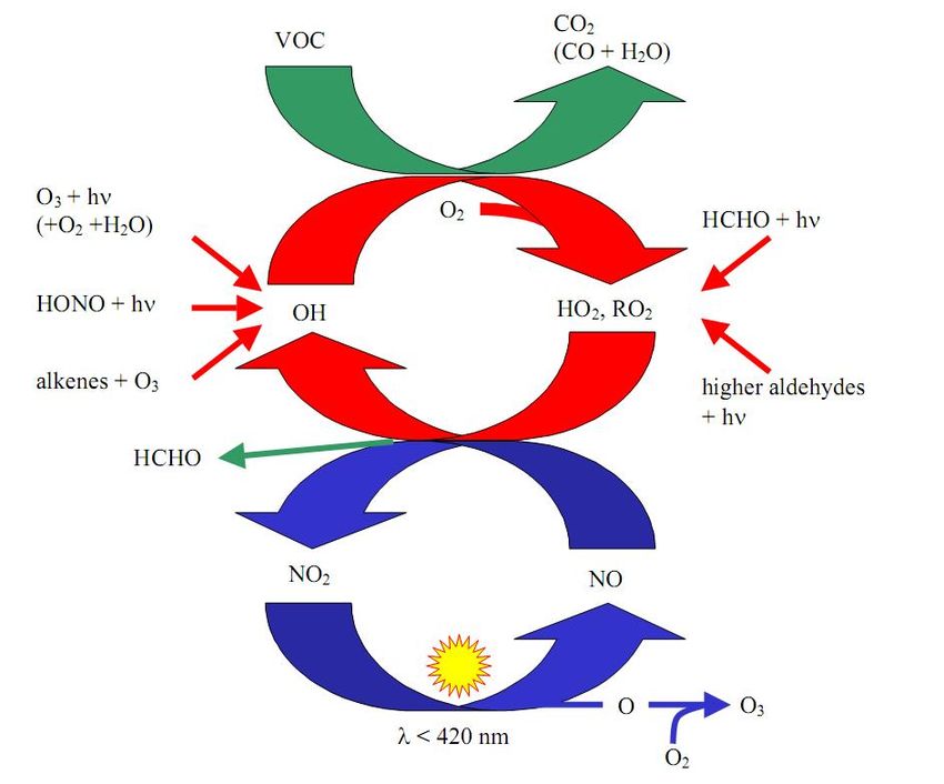
Contents

1 Background Information                                                                                                                        2
  1.1 The atmosphere . . . . . . . . . . . . . . . . . . . . . . . . . . . . . . . . . . . .                                                    2
  1.2 Measurements and dimensions . . . . . . . . . . . . . . . . . . . . . . . . . . . .                                                       2
  1.3 Composition of the air . . . . . . . . . . . . . . . . . . . . . . . . . . . . . . . .                                                    3

2 Stratospheric ozone                                                                                                                            5
  2.1 The importance of ozone in the stratosphere . . .                     . . . . .           .   .   .   .   .   .   .   .   .   .   .   .    5
      2.1.1 Vertical profile of ozone concentration . . .                   . . . . .           .   .   .   .   .   .   .   .   .   .   .   .    6
      2.1.2 The effects of harmful UV radiation . . . .                     . . . . .           .   .   .   .   .   .   .   .   .   .   .   .    6
  2.2 Photochemistry of ozone in the stratosphere . . .                     . . . . .           .   .   .   .   .   .   .   .   .   .   .   .    6
      2.2.1 Chapman cycle . . . . . . . . . . . . . . .                     . . . . .           .   .   .   .   .   .   .   .   .   .   .   .    6
      2.2.2 Catalytic ozone destruction . . . . . . . .                     . . . . .           .   .   .   .   .   .   .   .   .   .   .   .    7
      2.2.3 Anthropogenic influence on the total ozone                      column              .   .   .   .   .   .   .   .   .   .   .   .    7
      2.2.4 The Ozone hole . . . . . . . . . . . . . . .                    . . . . .           .   .   .   .   .   .   .   .   .   .   .   .    8

3 Nitrogen oxides                                                                                                                               10
  3.1 Health aspects of NO2 air pollution . . . . . . . . . . . . . . . .                                   .   .   .   .   .   .   .   .   .   10
  3.2 Sources and sinks of tropospheric NOx . . . . . . . . . . . . . .                                     .   .   .   .   .   .   .   .   .   11
  3.3 Photostationary state with ozone . . . . . . . . . . . . . . . . .                                    .   .   .   .   .   .   .   .   .   11
      3.3.1 NO2 Diurnal Cycle . . . . . . . . . . . . . . . . . . . . .                                     .   .   .   .   .   .   .   .   .   12
  3.4 Photochemical smog / deviation from the photostationary state                                         .   .   .   .   .   .   .   .   .   12

4 DOAS                                                                                                                                          15
  4.1 The Lambert-Beer Law . . . . . . . .      .   .   .   .   .   .   .   .   .   .   .   .   .   .   .   .   .   .   .   .   .   .   .   .   15
  4.2 The DOAS method . . . . . . . . . .       .   .   .   .   .   .   .   .   .   .   .   .   .   .   .   .   .   .   .   .   .   .   .   .   15
      4.2.1 Narrowband components . . .         .   .   .   .   .   .   .   .   .   .   .   .   .   .   .   .   .   .   .   .   .   .   .   .   16
      4.2.2 Broadband components . . . .        .   .   .   .   .   .   .   .   .   .   .   .   .   .   .   .   .   .   .   .   .   .   .   .   17
      4.2.3 Modified Lambert-Beer Law .         .   .   .   .   .   .   .   .   .   .   .   .   .   .   .   .   .   .   .   .   .   .   .   .   18
      4.2.4 The DOAS fit . . . . . . . . .      .   .   .   .   .   .   .   .   .   .   .   .   .   .   .   .   .   .   .   .   .   .   .   .   19
  4.3 Calculating trace gas concentrations .    .   .   .   .   .   .   .   .   .   .   .   .   .   .   .   .   .   .   .   .   .   .   .   .   19
      4.3.1 Active measurements . . . . .       .   .   .   .   .   .   .   .   .   .   .   .   .   .   .   .   .   .   .   .   .   .   .   .   20
      4.3.2 Zenith sky measurements . . .       .   .   .   .   .   .   .   .   .   .   .   .   .   .   .   .   .   .   .   .   .   .   .   .   20
      4.3.3 Multi-Axis-DOAS . . . . . . .       .   .   .   .   .   .   .   .   .   .   .   .   .   .   .   .   .   .   .   .   .   .   .   .   21
      4.3.4 Complex scenarios . . . . . .       .   .   .   .   .   .   .   .   .   .   .   .   .   .   .   .   .   .   .   .   .   .   .   .   22
  4.4 Background and noise . . . . . . . .      .   .   .   .   .   .   .   .   .   .   .   .   .   .   .   .   .   .   .   .   .   .   .   .   23
      4.4.1 Electronic offset . . . . . . . .   .   .   .   .   .   .   .   .   .   .   .   .   .   .   .   .   .   .   .   .   .   .   .   .   23
      4.4.2 Dark current . . . . . . . . .      .   .   .   .   .   .   .   .   .   .   .   .   .   .   .   .   .   .   .   .   .   .   .   .   24
      4.4.3 Noise . . . . . . . . . . . . . .   .   .   .   .   .   .   .   .   .   .   .   .   .   .   .   .   .   .   .   .   .   .   .   .   25
  4.5 Summary . . . . . . . . . . . . . . .     .   .   .   .   .   .   .   .   .   .   .   .   .   .   .   .   .   .   .   .   .   .   .   .   27

                                               IV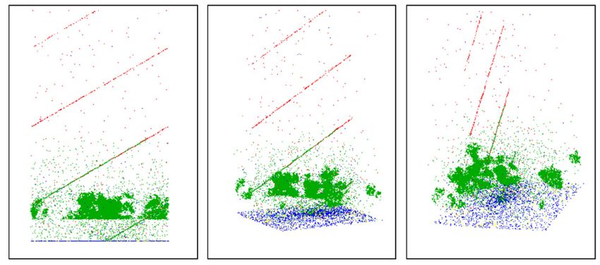
1

5 Experimental setup                                                                          28
  5.1 General setup . . . . . . . . . . . . . . . . . . . . . . . . . . . . . . . . . . . . . 28
  5.2 The spectrometer . . . . . . . . . . . . . . . . . . . . . . . . . . . . . . . . . . . 28

6 Software                                                                                     31
  6.1 DOASIS . . . . . . . . . . . . . . . . . . . . . . . . . . . . . . . . . . . . . . . . 31
  6.2 Python . . . . . . . . . . . . . . . . . . . . . . . . . . . . . . . . . . . . . . . . . 33
  6.3 Origin . . . . . . . . . . . . . . . . . . . . . . . . . . . . . . . . . . . . . . . . . 33

7 Course Instructions                                                                                           36
  7.1 Characterizing the instrumentation . . . . . . . . . . . . . . . . . .        .   .   .   .   .   .   .   36
      7.1.1 Offset . . . . . . . . . . . . . . . . . . . . . . . . . . . . . .      .   .   .   .   .   .   .   37
      7.1.2 Dark current . . . . . . . . . . . . . . . . . . . . . . . . . .        .   .   .   .   .   .   .   37
      7.1.3 Determining the instrument noise and total noise . . . . . .            .   .   .   .   .   .   .   37
      7.1.4 Calibrating the spectrometer . . . . . . . . . . . . . . . . . .        .   .   .   .   .   .   .   38
  7.2 Laboratory Measurements . . . . . . . . . . . . . . . . . . . . . . .         .   .   .   .   .   .   .   40
      7.2.1 Convolution of reference cross sections . . . . . . . . . . . .         .   .   .   .   .   .   .   40
      7.2.2 Recording a spectrum of the NO2 gas cell . . . . . . . . . .            .   .   .   .   .   .   .   41
      7.2.3 Determining the NO2 concentration in the gas cell . . . . . .           .   .   .   .   .   .   .   42
  7.3 Atmospheric Measurements . . . . . . . . . . . . . . . . . . . . . .          .   .   .   .   .   .   .   44
      7.3.1 Configuring the fit with a single measurement . . . . . . . .           .   .   .   .   .   .   .   44
      7.3.2 Automated evaluation of an entire day . . . . . . . . . . . .           .   .   .   .   .   .   .   46
  7.4 Multi Axis DOAS (MAX-DOAS) . . . . . . . . . . . . . . . . . . .              .   .   .   .   .   .   .   47
      7.4.1 Recording scattered light spectra at different elevation angles         .   .   .   .   .   .   .   47
      7.4.2 MAX-DOAS evaluation . . . . . . . . . . . . . . . . . . . .             .   .   .   .   .   .   .   47
  7.5 Before you leave... . . . . . . . . . . . . . . . . . . . . . . . . . . . .   .   .   .   .   .   .   .   47

8 Course Report                                                                                                 48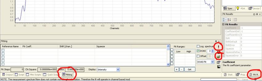
Chapter 1

Background Information

1.1     The atmosphere
An atmosphere 1 is a gas cover surrounding a star or a planet due to its gravitation. In the
following, we will only discuss the earth’s atmosphere. The atmosphere can be divided into
layers. The most common classification is linked to the temperature. According to this scheme,
the atmosphere is divided into the troposphere, the stratosphere, the mesosphere, the thermo-
sphere and the exosphere. The regions dividing two layers are called ’pause’, as in tropopause.
In the troposphere, the energy flow is dominated by incoming solar radiation heating up the
surface (Fig. 1.1). Sensible2 and latent3 heat are then transported from the ground up into the
troposphere, and thermal energy is converted into potential energy. The updraft of an airparcel
from the ground can be approximated by adiabatic cooling, which explains the temperature
decline of 6-10 K per km. This transport of latent heat drives the weather in the troposphere
and explains its turbulent behaviour. On the other hand, the energy balance in the stratosphere
is dominated by radiative heating due to absorption of incoming radiation by trace gases, for
example ozone. This leads to an increase of temperature with altitude and thus a stratification
of the airmasses, hence the term ’stratosphere’.

1.2     Measurements and dimensions
The concentration of a trace gas is the number of molecules in a volumetric unit. Its dimension
is typically [Molecules/cm3 ] or [µg/m3 ].

The mixing ratio is the relative amount of a trace gas as compared to the amount of air. The
units [ppm], [ppb] and [ppt] are common. Usually, the quantity is related to the volume ratio,
so the units are sometimes written as [ppmv], [ppbv], or [pptv].

For DOAS measurements, the column density  R plays an important role. This is the concentration
of a species integrated along a light path ρ(s)ds, and is typically given in molecules/cm2 .
The vertical column density gives the amount of molecules of a certain substance in the entire
atmosphere over a square centimeter on the ground. For ozone, the Dobson Unit [DU]4 has
become popular. 100 DU correspond to a vertical ozone column of 1 mm at 0°C and 1013.25
hPa. Typical vertical ozone columns in the atmosphere are between 300 and 400 DU. Therefore,
  1
    Greek atmos = haze
  2
    thermal energy that can be measured with a thermometer
  3
    Energy originating from evaporation on the ground or in the ocean.
  4
    1DU = 2,6·1016 Molecules/cm2

                                                    2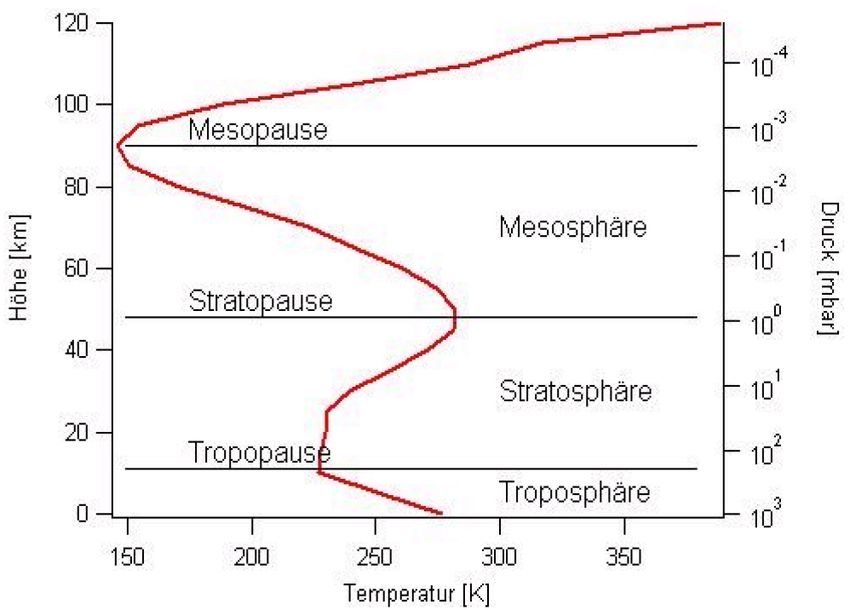
1.3. COMPOSITION OF THE AIR                                                                    3

                      Figure 1.1: Global annual mean energy budget. [30]

the total ozone in the atmosphere corresponds to a layer with 3-4 mm thickness when brought
to normal conditions.

1.3     Composition of the air
The main constituents of the air are oxygen, nitrogen and argon (see table 1.1). Water vapor can
have concentrations of between 0.02 % and 2.5 % in the troposphere. In the stratosphere, the
mixing ratio of water vapor is only about 3 - 4 ppm. All other gases together make up only 0.04
%, and are therefore called trace gases. Regarding the stable main constituents, the atmosphere
is well mixed and the number concentrations are basically proportional to the atmospheric
pressure profile. In first approximation, atmospheric pressure decreases exponentially with
altitude, approximately with a surface pressure of 1013 hPa and a scale height of 8 km. In
contrast to the main constituents, trace gas concentrations are significantly affected by complex
production and destruction cycles and may therefore vary strongly within space and time.

O4
The O4 molecule is the dimer of the oxygen molecule O2 . It can be formed when two oxygen
molecules collide. Therefore, its concentration is proportional to the square of the oxygen
concentration in the atmosphere. For this reason, its column is given in molecules2 /cm5 . Its
vertical profile is an exponential decrease with altitude with a scale height of approximately
4 km. Because the vertical profile of O4 concentration is well known, the measured column
densities can be used to gain insight into photon paths in the atmosphere, i.e. light path
enhancement due to aerosols and clouds [33].
4                              CHAPTER 1. BACKGROUND INFORMATION

      Figure 1.2: Atmospheric temperature profile and layering.

    Gas                            Symbol       Volume Fraction
    Nitrogen                         N2              78,08%
    Oxygen                           O2              20,95%
    Argon                            Ar               0,93%
    Water vapor                     H2 O             ca. 1%
    Carbon Dioxide                  CO2             358 ppmv
    Neon                             Ne            18,2 ppmv
    Methane                         CH4            1,75 ppmv
    Krypton                          Kr            1,14 ppmv
    Hydrogen                         H2             0,55ppmv
    Nitrous Oxide                   N2 O           0,31 ppmv
    Carbon Monoxide                  CO            0,11 ppmv
    Ozone                            O3            0,04 ppmv
    Chloroflourocarbons (CFCs)               (2,8 - 4,8)·10−4 ppmv

    Table 1.1: Chemical composition of the atmosphere at sea level.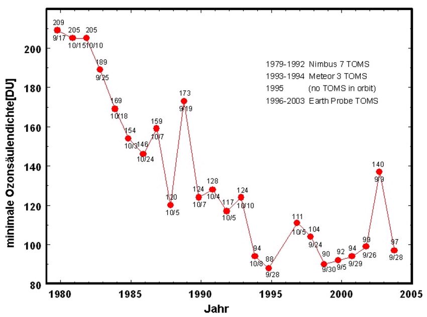
Chapter 2

Atmospheric chemistry I:
Stratospheric ozone

2.1      The importance of ozone in the stratosphere
The ozone molecule is composed of three oxygen atoms: O3 . In its gas phase, it is light blue. At
-111.9 °C, it condensates to an explosive, dark blue, magnetic liquid. At -192.5 °C, it crystalizes
to a dark violet mass. The dissociation at room temperature is slow, while it occurs explosively
if heated.
The average lifetime of an ozone molecule at 25 km altitude is about 1 hour. This lifetime is
determined by the photolysis frequency of ozone. However, the ozone concentration of a given
airmass changes slowly with time, as most oxygen atoms originating from ozone photolysis
quickly react back to ozone (see section 2.2). Therefore, it usually takes months or years to
significantly change the ozone concentration in a given airmass. This stands in contrast to the
quick reduction seen in the ozone hole formation discussed in section 2.2.4.
Ozone is a highly efficient absorber of UV radiation. Even though it is present only in such
small concentrations, it blocks a large part (95-99%) of the harmful (λ < 320 nm) UV radiation
at an altitude of 20 to 50 km. Therefore, the ozone layer is of great importance for life on earth.
The largest absorption of ozone occurs between 240 nm and 310 nm, as can be seen in figure
2.1.

Figure 2.1: Spectrum of incident solar radiation at the top of the atmosphere and at sea level.

                                                5
6 CHAPTER 2. STRATOSPHERIC OZONE
2.1.1 Vertical profile of ozone concentration
About 90% of the total ozone column is found in the stratosphere, the rest in the troposphere.
In mid latitudes, the ozone concentration at the ground is about 1·1012 molec/cm3 , while typical
concentrations in the stratosphere are 1·1013 to 2 ·1013 molec/cm3 (see figure 2.2, left panel).
The vertical profile of ozone is determined by the number of UV photons and the decreasing
number of oxygen molecules in the upper atmosphere. At high altitudes, the air is so thin
that the UV photons barely ever hit oxygen molecules and no atomic oxygen is formed. As
the density of the air increases with lower altitudes, the probability for O2 photolysis increases,
and the O3 mixing ratio follows this trend. The lower end of the ozone layer is reached, when
no more UV photons necessary for the formation of O3 are available, as they have all been
absorbed in higher layers.
Figure 2.2: Left: Ozone concentration vertical profile. Right: The enhancement of harmful UV
radiation is exponential with decreasing ozone columns, as described by the Beer-Lambert law of
absorption. This plot shows data measured in Antarctica between February 1991 and December
1992.
2.1.2 The effects of harmful UV radiation
The energy of shortwave UV radiation with wavelengths below 320 nm is enough to destroy
molecules, proteins and amino acids, which are the main constituents of organic matter. En-
hanced UV radiation directly increases the risk of skin cancer and biological mutation, and has
even been shown to directly influence marine biology and agriculture (see e.g. [12, 28, 29, 35]).
A decreasing ozone column in the stratosphere enables more UV radiation to reach the earth.
This relationship is not linear, as shown in figure 2.2, right panel.
2.2 Photochemistry of ozone in the stratosphere
2.2.1 Chapman cycle
Sidney Chapman [3] published the first simple theory about ozone in the stratosphere in 1930.
He postulated the ozone to be the result of a chemical equilibrium of 4 photochemical reactions.
At altitudes between 20 and 25 km, atomic oxygen is formed from the photolytical splitting of
oxygen molecules by shortwave UV radiation (λ < 242 nm).
O2 + hν → 2O (2.1)2.2. PHOTOCHEMISTRY OF OZONE IN THE STRATOSPHERE 7
Ozone is then formed by the recombination of the atomic oxygen with molecular oxygen.
O2 + O + M → O3 + M (2.2)
M is a chemically neutral molecule (e.g. N2 or O2 ) needed for conservation of momentum.
To reach an equilibrium ozone concentration, ozone destruction reactions are also necessary.
Chapman held the photolytic dissociation (λ < 1100nm) of ozone responsible:
O3 + hν → O2 + O(3 P) (2.3)
The formed oxygen atoms then either react according to equation 2.2 and form ozone again, or
they destroy an additional ozone molecule:
O3 + O → 2O2 (2.4)
These four reactions comprise the Chapman cycle. Chapman’s theory was correct, but the
measured ozone columns where always lower than his predicted ones, usually by about 40%.
Also, the height of the ozone maximum was incorrect.
2.2.2 Catalytic ozone destruction
Today we know that catalytic reactions 1 involving radicals of the groups HOx (H, OH, HO2 ),
NOx (NO, NO2 ) ClOx (Cl, ClO) and BrOx (Br, BrO) play a very important role in the destruc-
tion of ozone. The catalysts X greatly accelerate the ozone destruction previously mentioned
in equation 2.4.
X + O3 → XO + O2
XO + O → X + O2
Netto: O + O3 → O2 + O2
As catalysts are not removed from the cycle, they are available for further ozone destruction.
HOx and NOx can cycle through this reaction scheme 1000 to 10000 times before they are
removed from the atmosphere by chemical reaction or sedimentation. Because these reactions
are much faster than the reaction of O3 with O, the catalysts have a very strong influence on
stratospheric ozone chemistry, lowering the ozone concentrations when compared to the values
predicted by Chapman. By taking these catalytic reactions into account it was for the first time
possible to match predicted and measured vertical ozone profiles (see figure 2.3, left panel).
2.2.3 Anthropogenic influence on the total ozone column
Since the mid 80s, the average global total ozone columns have been decreasing. The total ozone
decrease after considering natural variations is about 5% per decade. This decrease can be seen
in mid latitudes, and is not restricted to the regions over Antarctica victimized by the ozone
hole (see section 2.2.4). The right panel of figure 2.3 shows the decrease in ozone after removing
all known natural variations from the trend. Ozone destruction by CFCs was detectable as early
as 1974. These gases are industrially produced compounds containing carbon (C), fluorine (F)
and chlorine (Cl). They found widespread use as cooling agents and gas propellant in spray
cans by the 1950s. CFC molecules are chemically inert in the lower troposphere, however upon
reaching the upper area of the ozone layer in about 30km altitude, CFCs are photolyzed by
1
Catalytic reactions are reactions that are controlled by a certain substance, the so-called catalyst. The
catalyst itself is not changed by the reaction.8 CHAPTER 2. STRATOSPHERIC OZONE
Figure 2.3: Left: The Chapman cycle alone predicts ozone mixing ratios approximately twice
as high as the measured values. Only by taking the catalytic ozone destruction into account the
measurements could be understood. Right: Decrease in global ozone after removing all known
natural variations.
shortwave UV radiation. The chlorine concentration of the atmosphere was increased by a
factor of 6 within a few decades by this process.
By the mid-1980s, scientists realised the influence of CFCs on ozone destruction. In 1987,
the industrialized nations signed the Montreal Protocol to reduce CFC emissions, followed by
several additional treaties thereafter. Figure 2.4 shows the global CFC production between
1986 and 1996.
Because of the long lifetimes of CFCs in the atmosphere (up to 100 years for some species), they
continue to act as catalysts in ozone destruction even though emissions have been drastically
reduced. In very recent years, the measured ozone hole has seemed to decrease in size and
intensity. However, it will still take several decades for the ozone layer to recover.2
Figure 2.4: Global CFC production by year for industrialized and developing nations.
2.2.4 The Ozone hole
In the middle of the 1980s, a maximum ozone loss of approximately 10% was predicted by
scientists due to destruction by CFCs. In October 1984, however, more than 40% of the ozone
in the ozone layer above Antarctica was destroyed. At the end of August, the ozone column
2
for details: Scientific Assessment of Ozone Depletion, WMO, 2010 at www.wmo.int2.2. PHOTOCHEMISTRY OF OZONE IN THE STRATOSPHERE 9
over Antarctica decreases rapidly and reaches a minimum in September. In November, the
values increase back to normal levels. Ozone is destroyed only in the altitude range between
12 and 30 km, as shown in figure 2.5. However, this is also where the ozone layer is normally
located. These findings could not be explained by dynamic processes alone. Instead, a complex
chemical mechanism was found to be responsible.
Figure 2.5: Left: Altitude profile of the ozone concenration measured over Antarctica in August
1997 and October 1997. Right: Time series of the annual minimum of the measured ozone
column density.
Chlorine and bromine reach the polar stratosphere in the form of transport-gases such as CFCs.
Here, they react to so-called reservoir gases. Chlorine and bromine are bound in these gases
and are removed from ozone destroying reactions. During the polar night, two processes then
combine to release the halogens. For one, a polar vortex forms in the stratosphere. Tropical
air masses are transported towards the poles and are deflected by the coriolis force. The large
temperature gradient present in the Antarctic winter from July to October causes the air to swirl
around the south pole in a stable stratospheric vortex, effectively shielding the south pole from
other adjacent air masses. In the absence of sunlight, the air in the Antarctic stratosphere then
cools to temperatures around -80 °C. At these very low temperatures, a second phenomenon
takes place. So-called Polar Stratospheric Clouds (PSC) are formed from ice, nitric acid and
some sulfuric acid. The extreme conditions necessary to form such clouds are only present
during the Antarctic winter in the absence of sunlight in altitudes between 15 and 25 km.
Once formed, the PSCs very effectively activate halogens through the following heterogeneous
reactions taking place on the ice surfaces.
XONO2 + H2 O → HNO3 + HOX (2.5)
XONO2 + HX → HNO3 + X2 (2.6)
X = Cl, Br.
Without the PSC-surfaces, these reactions would be very slow and therefore irrelevant. When
the sun now goes up in the Antarctic spring, the activated halogens act very effectively as
catalysts for ozone destruction. In the Arctic, the distribution of land masses prevents forming a
very strong polar vortex, therefore Arctic ozone hole is much less pronounced than the Antarctic
version. If all conditions remain the same, the ozone layer should recuperate by the middle of
the coming century. However, some aspects are still poorly understood. For example, when
ozone absorbs UV radiation, it heats the stratosphere. Ozone depletion therefore leads to a
cooling trend in the stratosphere, which could lead to an increased abundance of PSCs and
therefore even stronger ozone destruction. These and other questions are still being explored
to date.Chapter 3
Atmospheric chemistry II:
Nitrogen oxides
The Nitrogen oxides NO (nitric oxide) and NO2 (nitrogen dioxide) are together referred to as
NOx . They are one of the most problematic pollutants in urban areas not only in developing,
but also in industrialised countries. They are key species in the control of tropospheric ozone
production and by this play an important role in the formation of the so called ”Los Angeles
Smog” (see section 3.4). Moreover, the concentration of NOx has a strong influence on the
atmospheric level of hydroxyl radicals (OH), which initiates the degradation of most oxidizable
trace gases [7].
3.1 Health aspects of NO2 air pollution
Nitrogen dioxide is a brown, toxic gas: Mixing ratios over 20 ppm cause strong irritations of the
respiratory system including tickling of the throat, headaches, dizziness and eventually nausea.
At higher mixing ratios, it can lead to death (700 ppm after 30 minutes will be lethal). Inhaled
gas together with the humid mucosae creates nitric acid, which causes strong degradation of
the lungs capillaries (Air Liquide EG-safety data sheet). In addition to being a health hazard in
itself, NO2 is a precursor of a number of harmful secondary pollutants, including the formation
of inorganic particulate matter via HNO3 , and photo oxidants (e.g. ozone and PANs1 ). These
relationships are shown in figure 3.1.
Figure 3.1: Simplified relationship of NOx emission with formation of NO2 and other harmful
reaction products including O3 and particulate matter (PM2.5 ) [36].
1
peroxyacyl nitrates
103.2. SOURCES AND SINKS OF TROPOSPHERIC NOX 11
3.2 Sources and sinks of tropospheric NOx
The global emissions of NOx are caused by both human activities and natural processes. Table
?? shows the sources of NOx and their contribution to the global emissions. New highly resolved
satellite measurements allow to determine the global distribution of these NOx sources. Figure
3.2 depicts the 18 month mean of a satellite measurement of NO2 , which was recorded by
the SCIAMACHY instrument aboard the ESA satellite ENVISAT. Areas with high vertical
column densities correlate with urban areas and therefore anthropogenic sources. In fact more
than half of the global NOx emissions are man made. The major source of anthropogenic NOx
is the combustion of fossil fuels in industrial processes, power plants and traffic. The most
important mechanism for natural and anthropogenic production of NOx is the Zel’dovic cycle
[38] which describes the formation of thermal NO. The term thermal is chosen due to the
high activation energy necessary for reaction 3.2 of 318 kJ/mol. Therefore, NO is emitted from
combustion processes, e.g. in combustion engines (traffic) and from thermal power plants or
other industrial combustion processes.
O2 + M → O + O + M (3.1)
O + N2 ⇔ NO + N (3.2)
N + O2 ⇔ NO + O (3.3)
N + OH ⇔ NO + H (3.4)
Afterwards, NO2 can be produced via reaction 3.7. NOx is removed from the atmosphere mainly
by further oxidation. During the day hydroxyl radicals oxidize NO2 to nitric acid, which is then
removed from the atmosphere by wet (acid rain) and dry deposition:
NO2 + OH + M −→ HNO3 + M (3.5)
Another sink of NOx is the reaction of NO2 with ozone. Although the rate coefficient for this
reaction is relatively small, it cannot be neglected in areas with high ozone concentrations in
the absence of sunlight. During daytime this reaction plays no role because NO3 is rapidly
photolyzed. During the night, NO3 reacts with NO2 to form the anhydrite of nitric acid N2 O5 .
The major sink of tropospheric N2 O5 is the hydrolysis and subsequent wet or dry deposition
[19].
3.3 Photostationary state with ozone
Nitrogen dioxide is mainly a secondary pollutant. The oxidation to NO2 is explained by [16].
O(3 P) + O2 + M −→ O3 + M (3.6)
O3 + NO ⇐⇒ NO2 + O2 (3.7)
3
NO2 + hν (λ < 410 nm) −→ NO + O( P) (3.8)
Photolysis in reaction 3.8 does only occour at wavelenghts below 410nm. The third reaction
partner in 3.6 is required due to momentum conservation. The steady state concentrations of
O3 , NO and NO2 are linked by the Leighton ratio:
[NO] jNO2
= (3.9)
[NO2 ] kO3 +NO · [O3 ]
kO3 +N O is the reaction constant for eqn. 3.7. Since the photolysis rate changes with solar zenith
angle the Leighton ratio also changes during the course of the day. On a clear day, at noontime,
when the photolysis rate has its maximum of about jN O2 ≈ 8 × 10⁻³ s−1 the Leighton ratio has
its maximum and the lifetime of NO2 is about 2 min. At typical O3 mixing ratios of 30 ppb,
[N O]
[N O2 ]
is on the order of 1.12 CHAPTER 3. NITROGEN OXIDES
Figure 3.2: Satellite measurement of the NO2 vertical column densitiy averaged over the time
period from January 2003 to June 2004. The measurements have been performed with the
SCIAMACHY instrument aboard the ESA satellite ENVISAT. [1].
3.3.1 NO2 Diurnal Cycle
In an atmosphere that is free of volatile organic compounds (VOCs), NO2 , NO and O3 are in a
self contained diurnal cycle, which is strongly dependent on the sun’s UV light. In the morning,
the intensity of solar light increases. This leads to photodissociation of NO2 . But during the
day, NO and NO2 are in a photostationary balance (see reactions 3.6-3.8).
For the stratosphere, the mixing ratio of NO2 increases during the day, due to the dissociation
of N2 O5 to NO2 .
N2 O5 + hν → NO2 + NO3 (3.10)
NO3 splits up rapidly to NO2 or NO. This only happens during the daytime.
NO3 + hν → NO + O2 (3.11)
NO3 + hν → NO2 + O (3.12)
In the evening, the photolysis decreases and reaction 3.8 no longer creates NO. The result is
an increase of NO2 . At night NO2 forms N2 O5 again.
NO2 + O3 → NO3 + O2 (3.13)
NO3 + NO2 + M → N2 O5 + M (3.14)
3.4 Photochemical smog / deviation from the photosta-
tionary state
Since the first reports of photochemical smog in Los Angeles in the late 1940’s, extremely high
ozone levels have been measured in urban areas throughout the whole world. In Mexico City
ozone levels over 400 ppb have been reported. Photochemical smog is worst when high levels
of volatile organic compounds (VOCs) and NOx are emitted into a thermal inversion layer,
trapping them closely to the ground, and irradiated by sunlight during transport to downwind3.4. PHOTOCHEMICAL SMOG / DEVIATION FROM THE PHOTOSTATIONARY STATE13
Figure 3.3: Reaction cycles of tropospheric NOx and ozone in a polluted atmosphere. The
photostationary state of NOx is illustrated by the blue cycle. It is disrupted by the presence of
VOCs, which results in a net production of ozone. [31].
regions. This section discusses the mechanisms responsible for the creation of photochemical
smog.
The Leighton relation is only valid if reactions 3.6-3.8 describe the major sources and sinks of
NO2 and O3 . In the presence of VOCs, another reaction path for the conversion of NO to NO2
exists, without the destruction of O3 . The OH radical which usually initiates the reaction chain
is mainly formed by means of ozone photolysis:
O3 + hν (λ < 320 nm) −→ O(1 D) + O2 (3.15)
O(1 D) + H2 O −→ 2OH (3.16)
The reaction chain is started by the oxidation of a hydrocarbon (RH) which may be described
as
RH + OH −→ R + H2 O (3.17)
R + O2 −→ RO2 (3.18)
The peroxy radicals (RO2 ) and (HO2 ) react with NO and produce NO2 without destroying
ozone (see e.g. [2, 4, 20])
RO2 + NO −→ NO2 + RO (3.19)
RO + O2 −→ R′ CHO + HO2 (3.20)
HO2 + NO −→ NO2 + OH (3.21)14 CHAPTER 3. NITROGEN OXIDES
This scheme can be applied multiple times until the initial VOC is converted to CO2 or CO
and H2 O. Together with the reactions from 3.6-3.8 this can be written as an effective equation
for the ozone production:
RH + 4O2 + 2hν(λ < 410 nm) −→ R′ CHO + H2 O + 2O3 (3.22)
The reaction system is illustrated in figure 3.3 together with the most important sources of
OH, hydroxyl and peroxy radicals.Chapter 4
DOAS
Differential Optical Absorption Spectroscopy is a widely used technique in atmospheric research
for the detection of numerous trace gases, such as ozone, NO2 , formaldehyde, halogen radicals
(BrO, IO), water vapour, and many others [21, 22].
4.1 The Lambert-Beer Law
When electromagnetic radiation passes through matter, its intensity is reduced by absorption
and scattering. This process, called extinction, is described by the law of August Beer.
r
Figure 4.1: Light with the initial intensity I0 (λ) is emitted by a light source. After passing
through a volume of air containing an absorber with concentration ρ, the detector measures the
reduced intensity I(λ).
Let I0 (λ) be the intensity of a light beam at wavelength λ before entering the absorber, and
I(λ, L) the intensity after passing a layer of length L. Then the relationship between incident
and transmitted intensity is
I(λ, L) = I0 (λ) · exp(−σ(λ) · ρ · L) (4.1)
with σ being the absorption cross section and ρ the concentration of the trace gas. In general,
σ depends on pressure and temperature along the light path. Furthermore, the concentration
along the light path can vary. The Lambert-Beer law describes the absorption for n different
absorbers i:
Z LX n
!
I(λ, L) = I0 (λ) · exp − σi (λ) · ρi (s)ds (4.2)
0 i=1
4.2 The DOAS method
To determine the concentration of a particular trace gas in the atmosphere, it would, in prin-
ciple, be necessary to quantify all factors influencing the intensity I(λ) of a spectrum of light.
1516 CHAPTER 4. DOAS
In the laboratory, this can be achieved by removing the absorber from the light path. In the
atmosphere, however, where this is impossible, the multiple factors influencing the intensity
pose a dilemma. DOAS overcomes this challenge by using the fact that many processes in
radiative transfer show broad or even smooth spectral characteristics, while certain trace gases
exhibit narrowband absorption structures. The basic principle of DOAS is thus the separa-
tion of spectral structures in narrowband (varying strongly with wavelength) and broadband
components (varying slowly with wavelength) in differential spectra, so that changes in nar-
rowband absorptions can be detected (illustrated in figure 4.4). To use equation 4.2 in DOAS
measurements, it therefore has to be modified according to properties of radiative transfer in
the atmosphere and the measurement principles of DOAS instruments.
4.2.1 Narrowband components
Fraunhofer reference spectrum
The sun’s spectrum is highly structured (see figures 2.1 and 4.3, top). These structures must
be taken into account in a DOAS retrieval when using a passive instrument, i.e. when using
the sun as a light source. This is usually achieved by using a so-called Fraunhofer reference
spectrum I0 , which is a solar spectrum recorded under conditions in which the trace gases to
be investigated show little or no absorption.
Trace gas absorption
The primary quantity measured by DOAS instruments is the slant column density (SCD or S),
defined as the integrated concentration ρ of a trace gas i along the light path of length L:
Z L(λ)
SCD = Si (λ) = ρi (s)ds (4.3)
0
Each trace gas has its individual absorption cross section σi which serves as a spectral finger-
print. Several absorbers can be measured simultaneously even if their absorption features are
superimposed (see figure 4.2). By fitting these cross sections to recorded differential spectra,
SCDs are retrieved. If the Fraunhofer reference spectrum already contains absorption of a trace
gas, the SCD is often called differential Slant Column Density (∆SCD or ∆S ).
The Ring Effect
In 1961, J. Grainger and J. Ring [11] discovered that the the depth of the Fraunhofer lines
was smaller when examining scattered sunlight than when direct sunlight is observed. This was
attributed to inelastic rotational Raman scattering [32], which slightly changes the wavelength of
the scattered photon when the scattering occurs. This causes a ”filling in” of strong absorption
lines, as wavelengths on either side of the line are shifted into it. The magnitude of the so-called
Ring effect depends on the atmospheric path lengths of the photons entering the spectrometer.
The longer the path in the lower atmosphere where the air density is higher, the more likely
a Raman scattering event becomes. Therefore, the Ring effect is dependent e.g. on the solar
zenith angle, the cloud cover and the aerosol concentration in the atmosphere. To correct for
the Ring effect, a so-called Ring spectrum R(λ) is calculated (e.g. by DOASIS, figure 4.3).4.2. THE DOAS METHOD 17
Figure 4.2: UV/Vis absorption cross sections of atmospheric trace gases detectable by DOAS.
4.2.2 Broadband components
The light is affected by scattering and absorption on aerosol particles and cloud droplets (Mie
scattering) and by scattering on air molecules (Rayleigh scattering) 1 . The sum of both effects,
scattering and absorption, is referred to as extinction, εM and εR respectively. Both processes
εM and εR are elastic, i.e. the wavelength of the scattered photons remains constant during
the process. The Rayleigh scattering probability is proportional to λ−4 , so shorter wavelengths
are more likely to be scattered than long wavelengths. This is the reason why the sky appears
blue. Mie scattering is much less dependent on wavelength, so clouds and fog appear white, as
all wavelengths are equally scattered.
For the sake of integrity it should be noted that some trace gas cross sections also have broad-
band parts σi0 (λ) in addition to the narrowband parts mentioned above.
1
More precisely, we mean the Cabannes line of Rayleigh scattering. In a strict nomenclature, Rayleigh
scattering also includes rotational Raman lines (mentioned above), but these are treated separately in the
DOAS approach because of their effect on narrowband spectral structures. For clarity, see [37].18 CHAPTER 4. DOAS
Figure 4.3: An example of a Fraunhofer spectrum (top) and the Ring spectrum calculated from
it (bottom).
4.2.3 Modified Lambert-Beer Law
Considering sections 4.2.1 and 4.2.2, we expand equation 4.2:
!
X
I(λ, L) = I0 (λ) · exp −R(λ) − σi (λ) · Si (λ) · (4.4)
i
" !#
X
exp −L · (σi0 (λ) · ρi ) + εR (λ) + εM (λ)
i
Here, the first exponent contains all narrowband components and the second exponent contains
all broadband components. The separation of narrow and broadband absorption is illustrated
in figure 4.4 and the optical density is defined in the following section.
Figure 4.4: The principle of DOAS: The optical density τ is the result of narrow σi and broad-
band parts σi0 of an absorption cross section. Adapted from [22].4.3. CALCULATING TRACE GAS CONCENTRATIONS 19
4.2.4 The DOAS fit
Solving equation 4.4 for ln(I/I0 ) yields the optical density τ :
I(λ)
τ = ln (4.5)
I0 (λ)
X X
= −R(λ) − σi (λ) · Si (λ) − bk λk
i k
Here, bk λk is a polynomial to account for the second exponent of equation 4.4, which includes
P
all broad band features, as mentioned in section 4.2.2. R(λ) is the Ring spectrum and σi (λ)
and Si (λ) are the cross section and the slant column density of trace gas i, respectively. Apart
from atmospheric effects, the instrument itself also modulates the signal: The signal from light
reflected from elements in the spectrometer or the 0th or 2nd order of scattering from the
grating are called spectrometer stray light. If stray light intensity varies over the spectrum,
absorption bands at different wavelengths will be changed differently, i.e. the optical density
will be reduced more for some parts of the spectrum than for others. In order to account for
this, a so-called ’Offset’ polynomial IOf s (λ) can be added in the fitting procedure (see equation
4.6).
The idea of the DOAS fit is fairly simple. A model is used to construct an optical density
by taking into account all the physical effects the light entering the instrument undergoes.
This modelled optical density is then compared to the measured optical density. By varying
the physical parameters of the model (which include the trace gas column densities Si ), the
difference between model and measurement are minimized. When the minimum is reached, the
physical parameters of the model are assumed to represent those of the measurement.
Due to noise in the measurement (see section 4.4.3), the modelled optical density can never per-
fectly match the measured optical density. Therefore, the DOAS fit searches for the minimum
quadratic deviation (dependencies omitted for readability):
" #2
I0 + IOf s
X X
χ2 = ln −R− σi · Si − b k λk (4.6)
I i k
The unexplained remainder of the spectrum after minimisation (by varying the parameters Si
and bk ) is called the fit residual. The smaller the residual, the better the fit has succeeded in
modelling the trace gas absorption. Ideally, the residual is only composed of noise. In order
to detect a trace gas, its optical density needs to be larger than the residual. This criteria can
be used to estimate the detection limit for a particular species. Once the minimum was found,
the fit parameters Si represent the column densities of the individual trace gases.
4.3 Calculating trace gas concentrations
Depending on the measurement geometry, the column densities obtained with the evaluation
described above need to be interpreted in different ways. One way is the assumption of simplified
geometrical approaches (like in this experiment as described in the following sections), but in
more complex cases, extensive radiative transfer simulations have to be carried out (section
4.3.4). The observation geometry can be described by the solar zenith angle (SZA) θ (angle
between the zenith and the sun) and the telescope elevation angle α (angle between the horizon
and the viewing direction). The light path also depends on the solar relative azimuth angle
(SRAA), which is neglected here.20 CHAPTER 4. DOAS
Figure 4.5: Light path through the atmosphere in the case of small (left) and large (right) solar
zenith angle. With larger SZA, the light path through a stratospheric absorber is enhanced.
4.3.1 Active measurements
Active measurements are measurements with an active or artificial light source. In modern ap-
plications, often LEDs are used because of their well defined spectra. For active measurements,
the interpretation of the retrieved column densities is the simplest, because the light path is
clearly defined. It runs from the light source to the DOAS instrument. Dividing the column
density by the length of the light path directly yields the average trace gas concentration along
the light path. There are some similar applications, where the instrument points directly at
the sun or the moon (direct light measurements).
4.3.2 Zenith sky measurements
Zenith sky measurements are performed by looking straight up with a passive instrument. In
this geometry, the exact light path is unclear, but radiative transfer models can be used to
make a statistical prediction about the average path. In order to compare different SCDs
(which depend on the light paths), one can calculate the Vertical Column Density (VCD or V )
from the SCDs with the help of the so-called Air Mass Factor (AMF or A):
S(θ) 1
AMF = A(θ) := ≈ (4.7)
V cos(θ)
This approximation for the case of zenith sky measurements (valid for θ < 75) is illustrated in
figure 4.5. The Fraunhofer reference is typically taken at the minimal solar zenith angle around
noon. Therefore, the retrieved column densities are all relative to this value. The total SCD is
the sum of the ∆S and the column density already present in the Frauhofer spectrum SF .
S = ∆S + SF (4.8)
SF can be extracted with the help of a Langley Plot.
Langley plot
In a so-called Langley Plot, the measured ∆SCD is plotted as a function of the air mass factor
AMF. If the concentration of a measured trace gas is constant during the course of the day the
correlation between the ∆SCD and the AMF will be linear:4.3. CALCULATING TRACE GAS CONCENTRATIONS 21
S(θ)
V = (4.9)
A(θ)
∆S(θ) + SF
=
A(θ)
⇒ ∆S (A (θ)) = V · A (θ) − SF (4.10)
Here, θ is the solar zenith angle. If a constant concentration is assumed, the resulting plot
can be extrapolated to A = 0. Here, ∆S = −SF , and the column density in the Fraunhofer
reference spectrum can be retrieved (see figure 4.6). Note that the assumption of a constant
concentration is only valid for a few atmospheric absorbers, e.g. stratospheric ozone.
Figure 4.6: Two examples of Langley Plots. The left panel depicts the Langley Plot of an ozone
measurement. Extrapolation yields a Fraunhofer SCD of approximately 1019 molec/cm2 . The
panel on the right is a Langley Plot of a nitrogen dioxide measurement. Here, the concentration
is not constant during the course of the day, and the extrapolation does not yield a definite
value.
4.3.3 Multi-Axis-DOAS
The method of multi-axis DOAS (MAX-DOAS) strongly enhances the sensitivity for trace
gases located in the troposphere (for details, see [13]). When observing light with small eleva-
tion angles α (angle between the horizon and the viewing direction of the instrument), the light
paths through the lowermost atmospheric layers (and the SCDs of trace gases present there) are
strongly enhanced, as shown in figure 4.7. However, the light path through the stratosphere
does not change with elevation angle α. This offers the opportunity to distinguish between
stratospheric and tropospheric trace gases. This usually means recording the Fraunhofer ref-
erence spectrum in the zenith direction to minimize the light path through the lower layers of
the atmosphere. The airmass factor of a trace gas near the surface measured at an elevation
angle α can be approximated by:
1
A(α) ≈ (4.11)
sin(α)
However, light paths can become very complicated. For very small elevation angles, parts of the
observed light are scattered within the trace gas layer. Multiple scattering can occur for high
aerosol loads and under cloudy conditions. The geometric approximation (equation 4.11) is not
valid anymore under these conditions. An example of MAX-DOAS measurements is shown in
figure 4.8.22 CHAPTER 4. DOAS
Zenith
Stratosphere
Troposphere
Scattering
Tropospheric
a Absorber
Figure 4.7: Observation geometry of MAX-DOAS measurements.
SCD NO2 [molec/cm2]
Date 2003
Figure 4.8: NO2 SCDs measured with a MAX-DOAS instrument in Heidelberg. Different colours
indicate different telescope elevation angles. The SCD increases with decreasing elevation angle,
indicating the presence of NO2 near the surface. The U-shape of the diurnal profile is caused
by stratospheric NO2 .
4.3.4 Complex scenarios
In case of heavy aerosol loads, clouds and more complex measurement geometries, such as from
satellites, aircraft and ships, the approximations described above are no longer useful, because
the light path distributions can become very complex. For example, figure 4.9 illustrates two
basic cases for cloud influence on light paths. Light path distributions can be simulated by
radiative transfer models (figure 4.10). A Levenberg-Marquardt algorithm [17, 18, 24, 25] then
searches for minima in a χ2 landscape to retrieve radiative transfer model parameters (e.g.
aerosol load and trace gas concentrations) that best represent measured slant columns on the
one hand and knowledge about the atmosphere on the other hand. Examples of this approach
can be found in e.g. [8, 9, 14, 23, 33].4.4. BACKGROUND AND NOISE 23 Figure 4.9: Left: for clear sky, sun light is scattered by air molecules and aerosol particles towards the instrument. Center: diffusing screen effect: in the presence of thin clouds, a substantial fraction of the observed photons is scattered by the cloud; especially for the smaller elevation angles, this effect leads to an increase of the absorption path. Right: for optically thick and vertically extended clouds, multiple scattering can lead to a very large increase of the photon paths inside the clouds. [34] Figure 4.10: Three different perspectives of events simulated by McArtim, a 3D backward trajec- tory monte-carlo radiative transfer model, when observing a cumulus cloud at 670 nm. Green points represent cloud and aerosol particle scatter events, blue points depict absorption events. Ground scattering is shown in yellow and red dots symbolize Rayleigh scattering by air molecules and hint to the lines of sight of the instrument. [6] 4.4 Background and noise The spectra are collected by grating spectrometers with CCD detectors. The properties espe- cially of the detectors have to be taken into account in order to correctly record and process the spectra. 4.4.1 Electronic offset The offset is an electronic signal (e.g. an analogue voltage or current) which is added to the photon induced signal of each pixel for every exposure, because the AD-converter can not convert a negative input. The offset can therefore best be measured by recording an exposure at a very low exposure time with no light entering the spectrometer, as the measured signal will then consist almost exclusively of the offset signal. To minimize the noise, however, it is best to record many such scans in succession. For the Ocean Optics USB2000, e.g., typically 10000 scans at 3 ms (minimum exposure time of this spectrometer) exposure time are recorded (figure 4.11, left panel). As the offset is added to each scan, the resulting spectrum must first be scaled to the measurement spectrum by the number of scans before it is subtracted:
24                                                                                                                                                              CHAPTER 4. DOAS

                                                                                                                 NM eas
                                                                                              IOS (n) = I(n) −          · O(n)                                                                      (4.12)
                                                                                                                 NOS
Here, I(n) is the intensity measured at each pixel n, O(n) is the electronic offset, and N is the
number of scans with which the respective spectra were recorded.

                                       2 2 3
                                                                                                                                       4 0 0 0

                                                                                                                                       3 5 0 0
                                       2 2 2

                                                                                                                                       3 0 0 0

                                                                                                                  Intensität[counts]
     O ffs e t[c o u n ts /S c a n ]

                                       2 2 1                                                                                           2 5 0 0

                                                                                                                                       2 0 0 0

                                       2 2 0
                                                                                                                                       1 5 0 0

                                                                                                                                       1 0 0 0
                                       2 1 9
                                                                                                                                         5 0 0

                                       2 1 8                                                                                                  0
                                                                                                                                                  0   5 0 0    1 0 0 0              1 5 0 0   2 0 0 0
                                               0      5 0 0    1 0 0 0              1 5 0 0        2 0 0 0
                                                              P ix e ln u m m e r                                                                             P ix e ln u m m e r

Figure 4.11: Left: Offset spectrum recorded with an Ocean Optics USB2000 spectrometer. Most
pixels have an average offset of about 221 counts/scan. For a typical measurement with sat-
uration 75%, this is approximately 7% of the measured signal. Right: Dark current spectrum
recorded at an exposure time of 60 seconds with a USB2000 spectrometer. Most pixels register
a dark current of less than 4 counts per second, but a few so-called hot pixels register much
more.

4.4.2                                              Dark current
The dark current is caused by thermally excited electrons which pass the semiconductor band
gap due to Boltzmann statistics. Therefore, it strongly depends on the temperature of the
detector. In many spectrometers, the detectors are cooled to keep the dark current low. This
is especially important for modern UV-sensitive back-thinned detectors, as the dark current is
very high otherwise.
For a constant temperature, the dark current signal is proportional to the exposure time.
To measure the dark current it is therefore best to use a long exposure time and only one
exposure, so the offset is only added once. Of course no light should enter the spectrometer
during the measurement. For the USB2000, the maximum exposure time is 60 seconds (figure
4.11, right panel). After the measurement is recorded, the offset must be corrected and the
remaining signal is the dark current. When correcting for the dark current of a measurement
spectrum, the measured dark current must be scaled to the measurement exposure time before
it is subtracted:

                                                                                                                 tM eas
                                                                                              IDC (n) = I(n) −          · DOS                                                                       (4.13)
                                                                                                                  tDC
Here, I(n) is the intensity measured at each pixel n and DOS is the measured dark current
after correcting for the electronic offset. Before subtracting it, it is multiplied by the ratio of
the measurement exposure time and the dark current exposure time.
4.4. BACKGROUND AND NOISE 25
4.4.3 Noise
Two spectra will never be perfectly identical, even if they are recorded under identical condi-
tions. The reason for this is statistic noise in the photon signal and the detector background
signal and additionally systematic noise. The statistic noise can be quantified. A measurement
spectrum I = IB + IP is always composed of the background IB and the signal induced by the
incident photons IP . If multiple spectra are recorded under identical conditions, both contri-
butions will fluctuate around a mean value. Gaussian error propagation yields the following
equation for the total noise σ: q
σ= σB2 + σP2 (4.14)
The background noise σB is a property of the instrument and is therefore often referred to as
instrument noise. It is composed of fluctuations in the electronic offset and the dark current.
The photon noise σP is a fundamental physical phenomenon. For a given light intensity, the
number of photons in a certain time interval fluctuates. The number of registered photons is
then distributed according to the Poisson distribution: If M photons are registered on average
√
for a given time interval, the root mean square (RMS) of the obtained distribution will be M .
Spectroscopy instruments are designed so that the photon noise, not the instrument noise limits
the instrument precision (see figures 4.12 and 4.13).
To measure both the instrument and the photon noise, two spectra I1 and I2 are recorded in
quick succession, so the magnitude of the noise contributions in the two spectra can be assumed
to be equal. If the two spectra are then subtracted from each other, the noise of the difference
σD calculates to:
q
σD = σI21 + σI22 (4.15)
q
= 2σI2 (4.16)
1
⇒ σ Ii = √ σ D (4.17)
2
Note that this is the average noise over all pixels. The instrument noise can vary 20-30 %
from pixel to pixel in modern CCDs [27]. In order to be entirely precise one would therefore
have to characterise the instrument noise of each pixel separately, but since under reasonable
measurement conditions photon noise largely dominates the overall noise in a spectrum, it is
not necessary to deal with this ’noise of the instrument noise’. When collecting more and more
light, at a certain point all statistical noise is so small that only systematic noise remains in
the residual.26 CHAPTER 4. DOAS Figure 4.12: Noise measurements of a modern DOAS spectrometer. All statistical noise can theoretically be reduced indefinitely by adding up more photons (scans), but at a certain point systematic noise remains. [10] Figure 4.13: Calculation of the statistical noise contributions in a single readout of a modern CCD for different saturations. Photon noise is the largest statistical noise source for saturations > 5 %. [27]
4.5. SUMMARY 27
4.5 Summary
Each measured spectrum is composed of several superimposed signals:
1. Background. The background signal is the measured signal when no light enters the
spectrometer (section 4.4):
Electronic offset: Proportional to the number of scans recorded.
Dark current: Proportional to the exposure time.
2. Narrowband effects (section 4.2.1)
Fraunhofer spectrum: The Frauenhofer spectrum is the spectrum of the sun as it
arrives at the top of the earth’s atmosphere. It already contains many very strong
absorption structures. These are caused by light absorption by species in the sun’s
outer layers (photosphere).
Trace gas absorption: Trace gases in the atmosphere create characteristic absorption
structures in the measured spectra. The goal of the DOAS retrieval is to identify
and isolate these structures, which typically feature optical densities between 10−3
and 10−1 .
Raman scattering: Inelastic scattering filling in Fraunhofer lines.
3. Broadband effects (section 4.2.2)
Broadband absorption cross sections
Rayleigh & Mie scattering: Elastic scattering either by air molecules (Cabannes line
of Rayleigh scattering) or by small water droplets or particles called aerosols (Mie
scattering).
Spectrometer stray light (section 4.2.4)
4. Noise (section 4.4.3)
Instrument noise: Proportional to offset and dark current.
Photon noise: The noise of the number of photons at a given light intensity. Follows
Poisson statistics.
Systematic noise: Sources for systematic noise can be unexplained physical changes
in the instrument or in the atmosphere. Can you think of some sources of systematic
noise in this experiment?
The optical density τ calculated from two spectra I and I0 is then fitted with the least squares
method according to equation 4.6. The resulting slant columns S can be converted to vertical
columns and concentrations with knowledge about the light path, see section 4.3.You can also read