Greenhouse Gas Emissions Calculator for the Water Sector: User's Manual - Technical Memorandum No. 2
←
→
Page content transcription
If your browser does not render page correctly, please read the page content below
Technical Memorandum No. 2

Greenhouse Gas Emissions
Calculator for the Water Sector:
User’s Manual
Santa Ana Watershed Basin Study, California
Lower Colorado Region

U.S. Department of the Interior
Bureau of Reclamation                         August 2013

Mission Statements
The mission of the Department of the Interior is to protect and
provide access to our Nation’s natural and cultural heritage and
honor our trust responsibilities to Indian Tribes and our
commitments to island communities.

The mission of the Bureau of Reclamation is to manage, develop,
and protect water and related resources in an environmentally and
economically sound manner in the interest of the American public.
BUREAU OF RECLAMATION
Water and Environmental Resources Division (86-68200)
Water Resources Planning and Operations Support Group (86-68210)
Technical Services Center, Denver, Colorado

Technical Memorandum No. 86-68210-2013-03

Greenhouse Gas Emissions Calculator
for the Water Sector: User’s Manual
Santa Ana Watershed Basin Study, California
Lower Colorado Region

Prepared by:

Kristine Blickenstaff, Hydraulic Engineer

Peer reviewed by:

Laura Condon, Hydrologic Engineer

                                                               i
This page intentionally left blank.

ii
Contents
                                                                                                                   Page

Executive Summary .............................................................................................. 1
1.0 Introduction ..................................................................................................... 3
    1.1 Purpose, Scope, and Objective of Study .................................................... 3
    1.2 Literature Review....................................................................................... 3
    1.3 Legislation to Reduce GHG Emission ....................................................... 5
        1.3.1 Executive Order S-3-05 ..................................................................... 5
        1.3.2 Assembly Bill 32: The California Global Warming Solutions Act of
        2006............................................................................................................. 5
        1.3.3 Climate Change Scoping Plan ........................................................... 7
        1.3.4 Water Code Section 10541 ................................................................ 7
2.0 GHG Emissions Calculator Development .................................................... 9
    2.1 Methods...................................................................................................... 9
3.0 Using the GHG Emissions Calculator ......................................................... 11
    3.1 Data Entry ................................................................................................ 11
        3.1.1 Population Data............................................................................... 11
        3.1.2 Water Use Per Capita Data ............................................................. 12
        3.1.3 Water Supply Data .......................................................................... 13
        3.1.4 Potable Water Treatment Data ........................................................ 14
        3.1.5 Detailed Data .................................................................................. 15
    3.2 Results and Scenario Manager ................................................................. 15
4.0 SARW GHG Emissions and Mitigation Analysis ...................................... 17
    4.1 Location and Description of Study Area ................................................. 17
    4.2 Application of the GHG Emissions Calculator to the SARW ................. 19
5.0 Project Analysis Using GHG Emissions Calculator ................................. 25
    5.1 Wineville Regional Recycled Water Pipeline and Groundwater Recharge
    System Upgrades ............................................................................................ 25
        5.1.1 Background ..................................................................................... 25
        5.1.2 Results ............................................................................................. 26
    5.2 Forest First - Increase Stormwater Capture and Decrease Sediment
    Loading through Forest Ecological Restoration ............................................. 27
        5.2.1 Background ..................................................................................... 27
        5.2.2 Results ............................................................................................. 28
    5.3 Perris Desalination Program - Brackish Water Wells 94, 95 and 96 ....... 28
        5.3.1 Background ..................................................................................... 28
        5.3.2 Results ............................................................................................. 28
    5.4 San Sevaine Groundwater Recharge Basin.............................................. 29
        5.4.1 Background ..................................................................................... 29
        5.4.2 Results ............................................................................................. 30
    5.5 Vulcan Pit Flood Control and Aquifer Recharge Project ........................ 31
        5.5.1 Background ..................................................................................... 31
        5.5.2 Results ............................................................................................. 32
    5.6 Wilson Basins and Spreading Grounds.................................................... 33

                                                                                                                         iii
5.6.1 Background ..................................................................................... 33
5.6.2 Results ............................................................................................. 34
5.7 Peters Canyon Channel Water Capture and Reuse Pipeline .................... 35
5.7.1 Background ..................................................................................... 35
5.7.2 Results ............................................................................................. 36
5.8 Corona/Home Gardens Well Rehabilitation and Multi-Jurisdictional
Water Transmission Line Project.................................................................... 37
5.8.1 Background ..................................................................................... 37
5.8.2 Results ............................................................................................. 37
5.9 Commercial/Industrial/Institutional Performance-Based Water Use
Efficiency Program ......................................................................................... 39
5.9.1 Background ..................................................................................... 39
5.9.2 Results ............................................................................................. 40
5.10 Quail Valley Subarea 9 Phase 1 Sewer System Project ......................... 41
5.10.1 Background ................................................................................... 41
5.10.2 Results ........................................................................................... 42
5.11 Francis Street Storm Drain and Ely Basin Flood Control and Aquifer
Recharge Project ............................................................................................. 42
5.11.1 Background ................................................................................... 42
5.11.2 Results ........................................................................................... 43
5.12 Customer Handbook to Using Water Efficiently in the Landscape ....... 44
5.12.1 Background ................................................................................... 44
5.12.2 Results ........................................................................................... 44
5.13 Plunge Creek Water Recharge and Habitat Improvement ..................... 46
5.13.1 Background ................................................................................... 46
5.13.2 Results ........................................................................................... 46
5.14 Prado Basin Sediment Management Demonstration Project ................. 46
5.14.1 Background ................................................................................... 46
5.14.2 Results ........................................................................................... 47
5.15 Enhanced Stormwater Capture and Recharge along the Santa Ana River
......................................................................................................................... 47
5.15.1 Background ................................................................................... 47
5.15.2 Results ........................................................................................... 48
5.16 14th Street Groundwater Recharge and Storm Water Quality Treatment
Integration Facility .......................................................................................... 50
5.16.1 Background ................................................................................... 50
5.16.2 Results ........................................................................................... 51
5.17 Soboba Band of Luiseño Indians Wastewater Project ........................... 52
5.17.1 Background ................................................................................... 52
5.17.2 Results ........................................................................................... 53
5.18 Canyon Lake Hybrid Treatment Process ............................................... 53
5.18.1 Background ................................................................................... 53
5.18.2 Results ........................................................................................... 54
5.19 Recycled Water Project Phase I (Arlington-Central Avenue Pipeline) . 54
5.19.1 Background ................................................................................... 54
5.19.2 Results ........................................................................................... 54
iv5.20 Regional Residential Landscape Retrofit Program ................................ 54
5.20.1 Background ................................................................................... 54
5.20.2 Results ........................................................................................... 54
5.21 SAWPA Project Evaluation Summary .................................................. 56
6.0 References ..................................................................................................... 59
7.0 Appendix: Member Agency Baselines and Default Data .......................... 66
Figures
Figure 1: AB 32 Targets ......................................................................................... 6
Figure 2: Energy Consuming Process in the Delivery and Treatment of Water (red
not included in analysis) ................................................................................. 9
Figure 3: Screenshot of “Population” tab ............................................................. 12
Figure 4: Screenshot of “Water Use Per Capita” tab ............................................ 13
Figure 5: Screenshot of “Water Supply” tab......................................................... 14
Figure 6: Screenshot of “Potable Water Treatment” tab ...................................... 15
Figure 7: Screenshot of “Results” tab ................................................................... 16
Figure 8: SAWPA member agencies .................................................................... 18
Figure 9: Population for the Santa Ana River Watershed..................................... 19
Figure 10: Santa Ana Watershed water demand calculated for this study ........... 20
Figure 11: Baseline GHG emissions for the SARW ............................................. 20
Figure 12: Conservation for SAWR to meet a 20% reduction in GHG emissions
by 2020 (also referred to as 20x2020) .......................................................... 21
Figure 13: GHG emissions in the SARW resulting from 20x2020 in addition to
10% more self-supplied water by 2020 ........................................................ 22
Figure 14: GHG emissions in the SARW resulting from a 20% decadal reduction
in addition to 10% more self-supplied water by 2020 .................................. 23
Figure 15: SARW GHG emissions resulting from 20x2020 followed by a 40%
decadal reduction in GPCD (2030-2050) and decreases in imported water by
10% by 2020 and 2030 ................................................................................. 23
Figure 16: Comparison of GHG emissions resulting from conservation and
reduced imported water scenarios for the SARW......................................... 24
Figure 17: Wineville Project GHG Emission Comparison ................................... 27
Figure 18: San Sevaine Project GHG Emission Comparison ............................... 31
Figure 19: Vulcan Pit Project GHG Emission Comparison.................................. 33
Figure 20: Wilson Basins and Spreading Grounds Project GHG Emission
Comparison ................................................................................................... 35
Figure 21: Corona Project GHG Emission Comparison ....................................... 38
Figure 22: Commercial/Industrial/Institutional Performance-Based Water Use
Efficiency Program GHG Emission Comparison ......................................... 41
Figure 23: Francis Street Project GHG Emission Comparison ............................ 44
Figure 24: Customer Handbook to Using Water Efficiently in the Landscape
GHG Emission Comparison ......................................................................... 45
Figure 25: Enhanced Stormwater Capture and Recharge along the SAR Project
GHG Emission Comparison ......................................................................... 49
vFigure 26: 14th Street Project GHG Emission Comparison ................................. 52
Figure 27: Regional Residential Landscape Retrofit Program GHG Emission
Comparison ................................................................................................... 56
Figure A-1: Baseline GHG emissions for the SBVMWD .................................... 67
Figure A-2: Baseline GHG emissions for the WMWD ........................................ 68
Figure A-3: Baseline GHG emissions for the EMWD ......................................... 68
Figure A-4: Baseline GHG emissions for the IEUA ............................................ 69
Figure A-5: Baseline GHG emissions for the OCWD .......................................... 69
Figure A-6: Default energy data ........................................................................... 70
Figure A-7: California grid average electricity emissions factors ........................ 71
Tables
Table 1: Population and GPCD Water Use for the Wineville Project .................. 26
Table 2: No Action Water Supply Portfolio for the Wineville Project................. 27
Table 3: Population and GPCD Water Use for the San Sevaine Project .............. 30
Table 4: No Action Water Supply Portfolio for the San Sevaine Project ............. 30
Table 5: Population and GPCD Water Use for the Vulcan Pit Project ................. 32
Table 6: No Action Water Supply Portfolio for the Vulcan Pit Project ............... 32
Table 7: Population and GPCD Water Use for the Wilson Basins and Spreading
Grounds Project ............................................................................................ 34
Table 8: No Action Water Supply Portfolio for the Wilson Basins and Spreading
Grounds Project ............................................................................................ 35
Table 9: Population and GPCD Water Use for the Corona/Home Gardens Project
....................................................................................................................... 38
Table 10: No Action Water Supply Portfolio for the Corona/Home Gardens
Project ........................................................................................................... 38
Table 11: Population and GPCD Water Use for the
Commercial/Industrial/Institutional Performance-Based Water Use
Efficiency Program ....................................................................................... 40
Table 12: No Action Water Supply Portfolio for the
Commercial/Industrial/Institutional Performance-Based Water Use
Efficiency Program ....................................................................................... 40
Table 13: Population and GPCD Water Use for the Francis Street Project.......... 43
Table 14: No Action Water Supply Portfolio for the Francis Street Project ........ 43
Table 15: Population and GPCD Water Use for the Customer Handbook to Using
Water Efficiently in the Landscape Program ................................................ 45
Table 16: No Action Water Supply Portfolio for the Customer Handbook to Using
Water Efficiently in the Landscape Program ................................................ 45
Table 17: Population and GPCD Water Use for the Enhanced Stormwater Capture
and Recharge along the SAR Project ............................................................ 49
Table 18: No Action Water Supply Portfolio for the Enhanced Stormwater
Capture and Recharge along the SAR Project .............................................. 49
Table 19: Population and GPCD Water Use for the 14th Street Project ............... 51
Table 20: No Action Water Supply Portfolio for the 14th Street Project .............. 51
viTable 21: Population and GPCD Water Use for the Regional Residential
Landscape Retrofit Program ......................................................................... 55
Table 22: No Action Water Supply Portfolio for the Regional Residential
Landscape Retrofit Program ......................................................................... 55
Table 23: SAWPA 20 Project Finalists ................................................................ 57
viiAcronyms and Abbreviations °C degrees Celsius °F degrees Fahrenheit % percent ~ Approximately AB 32 Assembly Bill 32 AF acre-feet AFY acre-feet per year AR4 Fourth Assessment Report CFS cubic feet per second CO2e Carbon Dioxide Equivalent Corps U.S. Army Corps of Engineers DCP Downscaled Climate Projections DOE U.S. Department of Energy DWR California Department of Water Resources EMWD Eastern Municipal Water District EVMWD Elsinore Valley Municipal Water District GHG Greenhouse Gas GPCD gallons per capita per day IEUA Inland Empire Utilities Agency IPCC Intergovernmental Panel on Climate Change IRWM Integrated Regional Water Management km kilometer viii
MAF            million acre-feet

MAFY           million acre feet per year

Metropolitan   The Metropolitan Water District of Southern California

MGD            million gallons per day

mtCO2e         million metric tons of carbon dioxide equivalent

MWDOC          Municipal Water District of Orange County

OCWD           Orange County Water District

OWOW           One Water One Watershed

PPPI           Plunge Pool Pipeline

Reclamation    U.S. Department of the Interior, Bureau of Reclamation

SAR            Santa Ana River

SARP           Santa Ana River Mainstem Project

SARW           Santa Ana River Watershed

SAWPA          Santa Ana Watershed Project Authority

SBVMWD         San Bernardino Valley Municipal Water District

SECURE         Science and Engineering to Comprehensively Understand
               and Responsibly Enhance (Water Act)

SCAG           Southern California Association of Governments

SWE            Snow Water Equivalent

USGCRP         U.S. Global Change Research Program

WaterSMART     WaterSMART (Sustain and Manage America’s Resources
               for Tomorrow)

WMWD           Western Municipal Water District

WRMS           Water Resources Management System

                                                                        ix
This page intentionally left blank. x
Greenhouse Gas Emissions Calculator for the Water Sector: Users Manual – California
                                                   Santa Ana Watershed Basin Study

Executive Summary
The Santa Ana Watershed Basin Study (Basin Study) is a collaborative effort by
the Santa Ana Watershed Project Authority (SAWPA) and the Bureau of
Reclamation (Reclamation), authorized under the Sustain and Manage America's
Resources for Tomorrow SECURE Water Act (Title IX, Subtitle F of Public Law
111-11). The Basin Study complements SAWPA’s Integrated Regional Water
Management (IRWM) planning process, also known as their “One Water One
Watershed” (OWOW) Plan. It refines the watershed’s water projections, and
identifies potential adaptation strategies, in light of projected effects of climate
change. The Climate Change Analysis for the Santa Ana River Watershed
(SARW) is a contributing section to the Basin Study. The Greenhouse Gas
(GHG) Emissions Calculator was developed as a tool to support the Climate
Change Analysis. It was developed to evaluate mitigation strategies, while the
Climate Change Analysis focused primarily on adaption and vulnerability
analysis. Development of the tool began in 2012 and was completed in August
2013.

This report explains the methods used to develop the calculator and provides
instructions on how to use it by introducing examples. The examples focus on the
SARW to show how to develop a GHG emissions baseline, evaluate what it
would take to meet specific GHG emission reduction goals, and illustrate how the
GHG Emissions Calculator can be used to analyze projects. Chapter 1 provides
an introduction to the project, a literature review, and a summary of California’s
GHG legislation. The methods used in the GHG Emissions Calculator can be
found in Chapter 2. A guide showing users what data is needed and how to enter
that data can be found in Chapter 3. Chapter 4 provides an introduction to the
SARW, the GHG emission baseline for the SARW, discusses varies scenarios to
reduce GHG emissions, and compares those reduction scenarios. In Chapter 5
SAWPA’s 20 finalist for the Integrated Regional Water Management (IRWM)
funding were analyzed using the GHG Emissions Calculator.

The GHG Emission Calculator is a decision-making tool that can be used to
explore the links between water resources, energy, and GHG emissions. It can be
used to determine water supply and energy demands for the study area, in addition
to GHG emissions from 1990 to 2050. It can be used to analyze a study area
ranging from a city block to an entire watershed, regardless of the level of
detailed data available. The GHG Emissions calculator is a vital tool for decision
makers when developing water supply plans for the future. It is also equipped to
evaluate long term GHG emission reduction potential for new projects that will
alter the water supply portfolio.

                                                                                   1
Greenhouse Gas Emissions Calculator for the Water Sector: Users Manual – California
Santa Ana Watershed Basin Study
This page intentionally left blank.
2Greenhouse Gas Emissions Calculator for the Water Sector: Users Manual – California
Santa Ana Watershed Basin Study
1.0 Introduction
1.1 Purpose, Scope, and Objective of Study
The Santa Ana Watershed Basin Study (Basin Study) is a collaborative effort by
the Santa Ana Watershed Project Authority (SAWPA) and the Bureau of
Reclamation (Reclamation), authorized under the Sustain and Manage America's
Resources for Tomorrow SECURE Water Act (Title IX, Subtitle F of Public Law
111-11). The Basin Study complements SAWPA’s Integrated Regional Water
Management (IRWM) planning process, also known as their “One Water One
Watershed” (OWOW) Plan. It refines the watershed’s water projections, and
identifies potential adaptation strategies, in light of projected effects of climate
change. The Climate Change Analysis for the Santa Ana River Watershed
(SARW) is a contributing section to the Basin Study. The Greenhouse Gas
(GHG) Emissions Calculator was developed as a tool to support the Climate
Change Analysis. It was developed to evaluate mitigation strategies, while the
Climate Change Analysis focused primarily on adaption and vulnerability
analysis. Development of the tool began in 2012 and was completed in August
2013.
Climate change threatens California’s natural environment, economic prosperity,
public health, and quality of life. Recognizing the need for action, California has
put in place ambitious GHG emission reduction goals. Recently California passed
legislation requiring drastic reduction in GHG emissions. In order to meet these
reduction goals a new methodology was required to determine GHG emissions in
the past, present, and future. The GHG Emissions Calculator, developed by
Reclamation, is a tool that fills that need.
The GHG Emission Calculator is a decision-making tool that can be used to
explore the links between water resources, energy, and GHG emissions. It can be
used to determine water supply and energy demands for the study area, in addition
to GHG emissions from 1990 to 2050. The GHG Emissions calculator is a vital
tool for decision makers when developing water supply plans for the future. It is
also equipped to evaluate long term GHG emission reduction potential for new
projects that will alter the water supply portfolio.
1.2 Literature Review
Water resource managers are currently faced with the challenge of developing
sustainable methods for adaptation and mitigation to climate change. Demands
for treatment and transportation of water are increasing globally due to
3Greenhouse Gas Emissions Calculator for the Water Sector: Users Manual – California Santa Ana Watershed Basin Study developments in industrial, agricultural and domestic water use, as well as water quality regulation (King et al., 2008). Large increases in energy use in the water sector are driven by rising demand for food and bio-fuels, and their international trade, driving up irrigated cropland and cropping intensity (Curlee et al., 2003; DOE, 2006). Worldwide food production is expected to increase 50% by 2030, at the cost of considerable increase of irrigated area and water use (Bruinsma, 2003). This estimate excludes the effects of climate change, which in many cases will put further pressure on water resources (IPCC Secretariat, 2008). The demand for irrigation water is likely to increase as temperatures increase and precipitation become more variable (Doll, 2002; Bruinsma, 2004; Fischer et al., 2007; Rosenberg et al., 2003; Xiong et al, 2010). With increased irrigation, additional development of groundwater is highly likely. Declining groundwater will compound energy use, as deeper wells require more carbon-intensive electrical pumps. Across the United States, the demand for electricity is colliding with the need for healthy and abundant fresh water. Large amounts of electricity are required to develop, treat, and transport the water supply for the growing population of the United States, currently 315.5 million (U.S. Census Bureau, 2013). However, in order to produce the requisite electricity to supply our water needs, a large amount of water is needed to produce that energy, regardless of the source (Bauer, 2009; Sovacool, 2009; DOE, 2011). The interdependence of water and energy has long been referred to as the water-energy nexus. Although there is a potential for a shortage of either water or energy to limit the production of the other, the majority of research has been focused on water as the limiting factor (Alley et al., 1999; EPRI, 2002; DOE, 2006; Dziegielewski et al., 2006; Amons, 2007; ACEEE, 2011). Very little research has been done on what would happen if energy were to become the limiting factor, let alone adaptation and mitigation strategies (Racoviceanu, 2007). There has been some research on greenhouse gas emissions (GHGE) from the various water supply methods. A study done by Stokes et al., in 2006 showed that for most U.S. utilities analyzed, higher GHG emissions result – by a factor of 1.5 to 2.4 percent – from desalination than either recycled water use or importation. Slightly more research has been done focusing on GHG emissions from wastewater systems (Racoviceanu et al., 2009; Shehabi et al., 2012). A study published by the River Network in 2009 provides a qualitative analysis of GHG emissions from energy use in the water sector, developing a baseline estimate of water related energy use in the U.S., as well as a comparative overview of the energy embedded in different water supplies and end uses. Connections between Energy use and GHG emissions are poorly understood and have only been partially considered in water management and planning. 4
Greenhouse Gas Emissions Calculator for the Water Sector: Users Manual – California
                                                   Santa Ana Watershed Basin Study

Growing populations are creating a higher water demand, and in areas where
water is already scarce accelerated research will be required to help develop
sustainable mitigation and adaptation scenarios to climate change while still
meeting the demand. Research on planning and mainstream adaptation in water
management is growing (Subak, 2000; Charlton & Arnell, 2011; Farley et al.,
2011). However, few studies consider, in detail, the energy and emission
implications of adaptation measures, and there is a need to achieve better linkage
between adaptation and mitigation. Comparisons between the few studies that
have been conducted are challenging due to the lack of a common carbon
assessment methodology for the water sector (Frijns, 2011). Consideration of
alternative water supply systems, treatment technologies, or water allocation may
have a tendency to overlook the carbon cost. This is particularly the case in the
absence of regulatory pressure.

1.3 Legislation to Reduce GHG Emission
National and international actions are necessary to fully address the issue of
climate change. However, action taken by California to reduce GHG emissions
has and will continue to have far-reaching effects by encouraging other states, the
federal government, and other countries to act. The following section is a
summary of State legislation and policy that California has passed in order to
reduce GHG emissions.

1.3.1 Executive Order S-3-05
California began to lead the charge to reduce GHG emissions back in 2005 when
Governor Schwarzenegger passed Executive Order S-3-05 (EO S-3-05). EO S-3-
05 laid the groundwork for establishing the California Environmental Protection
Agency’s (Cal EPA) Climate Action Team (CAT) and developed GHG reduction
targets for California including:
    • Reduction of GHG emissions to 2000 levels by 2010
    • Reduction of GHG emissions to 1990 levels by 2020
    • Reduction of GHG emissions to 80% below 1990 levels by 2050
CAT established a sub-group known as the Water-Energy group, or WET-CAT,
to monitor the progress of GHG emission reduction efforts and coordinate GHG
mitigation strategies.

1.3.2 Assembly Bill 32: The California Global Warming Solutions Act
of 2006
The passing of California’s Assembly Bill 32: The Global Warming Solutions Act
(AB 32) codified the GHG emission reduction targets set forth in EO S-3-05. A
number of studies noted that climate change threatens California’s natural
environment, economic prosperity, public health, and quality of life (CEC, 2005;
Lofman et al., 2006; AB 32, 2006). Recognizing the need for action, California
put in place ambitious emission reduction goals in the form of AB 32. By
requiring, in law, a reduction in GHGE, California set the stage to transition to a
sustainable, clean energy future, while puting climate change on the national
                                                                                   5
Greenhouse Gas Emissions Calculator for the Water Sector: Users Manual – California Santa Ana Watershed Basin Study agenda and spurring action by many other states. For example, in 2008 Massachusetts Governor Deval Patrick signed into law that state’s Global Warming Solutions Act that mirrors AB 32. Also in 2008, the government of the United Kingdom launched a new strategy for the water sector that includes the same GHGE targets as AB 32 (Stationary office, 2008). AB 32 directly links anthropogenic GHGE and climate change, provides a timeline for statewide GHGE reduction, requires quantitative accounting of GHGE, and enforces disclosure of GHGE from every major economic sector in the state. AB 32 requires that every major sector in California reduce its GHGE to the 1990 levels by 2020, and to 80% below the 1990 levels by 2050 (see Figure 1). These targets were developed from the levels of reduction climate scientists agree are required to stabilize our climate (IPCC Tech Paper III, 1997). The 2020 Statewide baseline, shown in Figure 1, represents the projected GHGE out to 2050 if no action is taken. GHGE are measured in carbon dioxide equivalent (CO2e), which represents the equivalent amount of CO2 that would cause the same effects as the greenhouse gas being represented. It has been argued that, the only way for the water sector to achieve these ambitious GHGE reduction goals is to drastically reduce its energy use (Friedrich et al., 2007). This brings up one of the major issues when accounting for GHG emissions in the water sector – the majority of GHG emissions come from electricity use for pumping, treating, and transporting water. GHG emissions from electricity used in the water sector are accounted for in the electricity sector, resulting in double accounting. The Scoping Plan, summarized below, addresses this issue by categorizing the water sector’s GHG reductions as a factor of safety. Figure 1: AB 32 Targets 6
Greenhouse Gas Emissions Calculator for the Water Sector: Users Manual – California
                                                   Santa Ana Watershed Basin Study

1.3.3 Climate Change Scoping Plan
The Climate Change Scoping Plan, developed pursuant to AB 32, recommends
specific strategies for each sector to achieve the GHG emission reduction goals
set out by AB 32. The scoping plan, adopted in 2008, addresses double
accounting by the water sector, and lays out six areas of focus to encourage the
water sector to do its part.
    • Water use efficiency
    • Water recycling
    • Water system energy efficiency
    • Reuse of urban runoff
    • Increased renewable energy production
    • Public goods charge for water
The Scoping Plan identifies water use as a sector requiring significant amounts of
energy. It sets goals to use cleaner energy to treat and move water and to work
towards higher efficiency.

1.3.4 Water Code Section 10541
California Water Code Section 10541 requires that all Integrated Regional Water
Management (IRWM) Plans address climate change by evaluating the
adaptability of water management systems to climate change and by considering
GHG emissions of all identified programs and projects.

                                                                                   7
Greenhouse Gas Emissions Calculator for the Water Sector: Users Manual – California
Santa Ana Watershed Basin Study
This page intentionally left blank.
8Greenhouse Gas Emissions Calculator for the Water Sector: Users Manual – California
Santa Ana Watershed Basin Study
2.0 GHG Emissions Calculator
Development
2.1 Methods
The methods used account for embodied energy and the subsequent GHG
emissions of water consumption in a study area. Figure 2 illustrates the different
energy consuming processes involved in the delivery and treatment of water.
End-use of water (e.g. the energy used to heat water in the home) is not
considered in this analysis due to the user specific data that would be required. To
accurately inventory emissions, the energy intensity of each of the processes
shown in Figure 2, and the volume of water passing through each, is required. The
level of site specific data that is known will define the accuracy of the results
when determining the GHG emissions from the water sector.
Figure 2: Energy Consuming Process in the Delivery and Treatment of
Water (red not included in analysis)
This methodology depends on study area specific energy consumed per unit of
water for each process in Figure 2. If site specific information is not available,
southern California defaults are used. Default utility specific emission factors
were obtained from the California Climate Action Registry Power/Utility Protocol
reports. Annual average electricity emission factors came from the California Air
Resources Board Greenhouse Gas Inventory (2007), and eGRID (2009).
Equation 1 depicts how total annual CO2e emissions are calculated:
9Greenhouse Gas Emissions Calculator for the Water Sector: Users Manual – California
Santa Ana Watershed Basin Study
Annual CO2e emissions = Extraction + Conveyance + Treatment +
Distribution…….Eq. 1
Where:
Extraction =
Conveyance =
Treatment =
Distribution =
The GHG Emissions Calculator detailed here was developed by Reclamation to
allow users to implement this method to easily and quickly evaluate how water
management decisions affect water demand, energy use, and GHG emissions.
10Greenhouse Gas Emissions Calculator for the Water Sector: Users Manual – California
Santa Ana Watershed Basin Study
3.0 Using the GHG Emissions
Calculator
3.1 Data Entry
The consumption of water by a community’s residents and businesses can have
significant GHG implications depending on the source, treatment, distance, and
topography traversed. Incorporating the relationship between water and energy
consumption in a GHG inventory allows a community to use water conservation
and policy measures as a GHG emissions reduction strategy. This tool allows the
user to estimate GHG emissions from 1990-2050 regardless of data availability.
It can be used with three levels of data: Required Data, Suggested Data, and
Detailed Data, or any combination of the 3. Yellow cells in each worksheet take
user input, blue cells are calculated values, and tan cells provide detailed
instructions.
The only required data is population of the area being analyzed for 1990, 2000,
2010, and present. Suggested data includes the following site specific data for the
study area:
• Projected population data for 2020, 2030, 2040, and 2050
• Water use per capita for 1990, 2000, 2010, present, 2020, 2030, 2040, and
2050
• Percentage each of groundwater, State Water Project, and Colorado River
Water
Detailed site specific data should be used when it is available, but default southern
California data will fill any data gaps. The following detailed data can be entered
on either a monthly or annual level under the blue tabs.
• State Water Project data (ac-ft)
• Colorado River Water data (ac-ft)
• Potable water treatment flow (gal for monthly data, MG for annual)
• Potable water treatment energy data (KWh)
• Groundwater elevation data (ft)
• Groundwater energy data (KWh)
3.1.1 Population Data
Required data should be entered in the spreadsheet marked with the “Population”
tab in cells F1-F4, as seen in the screenshot found in Figure 3. If population
projections for 2020, 2030, 2040, and 2050 are know they can be entered in cells
F8-I8, also shown in Figure 3. If exact population projections are not known,
11Greenhouse Gas Emissions Calculator for the Water Sector: Users Manual – California
Santa Ana Watershed Basin Study
default southern California projected growth rate will be used. If the user would
prefer to evaluate population projection scenarios they can be entered as decadal
percent growth or annual percent growth in cells F16-I16 and F24-I24
respectively (see Figure 3). Only one of the methods of entering projected
population can be used at a time.
1990 Population: 4,200,000
2000 Population: 5,094,600
Required Data
2010 Population: 5,900,000
Current Population: 6,086,666 Projected
Population
Known Population
1990 2000 2010 2020 2030 2040 2050
Population 4,200,000 5,094,600 5,900,000
Decadal Growth Rate 21% 16% 0% 0% 0% 0%
Annual Growth Rate 2.13% 1.58% 0.00% 0.00% 0.00% 0.00%
Source:
Known Decadal Growth Rate
1990 2000 2010 2020 2030 2040 2050
Population 4,200,000 5,094,600 5,900,000 5,900,000 5,900,000 5,900,000 5,900,000
Decadal Growth Rate 21% 16%
Annual Growth Rate 2.13% 1.58% 0.00% 0.00% 0.00% 0.00%
Source:
Known Average Annual Growth Rate
1990 2000 2010 2020 2030 2040 2050
Population 4,200,000 5,094,600 5,900,000 5,900,000 5,900,000 5,900,000 5,900,000
Decadal Growth Rate 21% 16% 0% 0% 0% 0%
Annual Growth Rate 2.13% 1.58%
Source:
Figure 3: Screenshot of “Population” tab
3.1.2 Water Use Per Capita Data
Water use per capita data should be entered in the spreadsheet marked with
“Water Use Per Capita”. Current and historic data should be entered in cells F2-
F5. If per capita water use projections for 2020, 2030, 2040, and 2050 are known,
they can be entered in cells F9-I9. If exact per capita water use is not known,
default southern California data will be used. If the user would like to evaluate
various conservation scenarios, that can be done in the “Water Use Per Capita”
tab using precise goals, a decadal percent reduction, or annual percent reduction
in cells F9-FI, F17-I17, or F25-I25 respectively (see Figure 4). Only one of the
methods of entering per capita water can be used at a time.
12Greenhouse Gas Emissions Calculator for the Water Sector: Users Manual – California
Santa Ana Watershed Basin Study
Current Per Capita Water Use (gpd):
1990 Per Capita Water Use: Past and Current Per
2000 Per Capita Water Use: Capita Water Use
2010 Per Capita Water Use:
Projected Per Capita Water Use
Projected Per Capita Water Use
1990 2000 2010 2020 2030 2040 2050
Per Capita Water Use (gpd) 209 209 209
Decadal Conservation Rate 0.00% 0.00% 0.00% 0.00% 0.00% 0.00%
Annual Conservation Rate 0.00% 0.00% 0.00% 0.00% 0.00% 0.00%
Source:
Projected Annual Conservation Rate
1990 2000 2010 2020 2030 2040 2050
Per Capita Water Use (gpd) 209 209 209 209 209 209 209
Decadal Conservation Rate 0.00% 0.00%
Annual Conservation Rate 0.00% 0.00% 0.00% 0.00% 0.00% 0.00%
Source:
Projected Annual Conservation Rate
1990 2000 2010 2020 2030 2040 2050
Per Capita Water Use (gpd) 209 209 209 209 209 209 209
Decadal Conservation Rate 0.00% 0.00% 0.00% 0.00% 0.00% 0.00%
Annual Conservation Rate 0.00% 0.00%
Source:
Default per capita water use for So Cal: 209
Figure 4: Screenshot of “Water Use Per Capita” tab
3.1.3 Water Supply Data
Water supply data should be entered in the spreadsheet marked “Water Supply”.
Current data should be entered as percentages in cells F2-F5. Self-supplied water
should not be entered; rather it is calculated by subtracting the other supply data
from the total. If historic water supply volumes are known for groundwater, State
Water Project (SWP), and Colorado River Aqueduct (CRA) those should be
entered in cells C9-E9, C15-E15, and C21-E21, respectively. Water supply
portfolio projections for 2020, 2030, 2040, and 2050 can be entered as percent to
total water supply in cells F10-I10, F16-I16, and F22-I22 for groundwater, SWP,
and CRA respectively (see Figure 5). If no data is entered for water supply, the
southern California defaults will be used.
13Greenhouse Gas Emissions Calculator for the Water Sector: Users Manual – California
Santa Ana Watershed Basin Study
Percent Groundwater Use:
Percent State Water Project: Current Water Supply %
Percent Colorado River Water:
Percent Self-Supplied Water Use: 100% Projected Water Supply %
Groundwater
1990 2000 2010 2020 2030 2040 2050
Groundwater Production (AFY) 242,241 271,032 307,252 343,471
Percentage of water supplied 17.00% 17.00% 17.00%
Source:
State Water Project
1990 2000 2010 2020 2030 2040 2050
Imported Water (AFY) 1,082,960 1,211,672 1,373,595 1,535,519
Percentage of water supplied 38.00% 38.00% 38.00%
Source:
Colorado River Aqueduct
1990 2000 2010 2020 2030 2040 2050
Imported Water (AFY) 0 0 0 0
Percentage of water supplied 38.00% 38.00% 38.00%
Source:
Total Water Use (AFY) 983,261 1,192,696 1,381,248 1,424,948 1,594,305 1,807,362 2,020,420
Default groundwater use for So Cal: 17%
Default surface water use for So Cal: 76%
Default self-supplied water use for So Cal: 7% Historic Water
Supply Volume
Figure 5: Screenshot of “Water Supply” tab
3.1.4 Potable Water Treatment Data
Potable water treatment data should be entered in the spreadsheet marked with
“Potable Water Treatment”. Current and historic data should be entered in cells
F2-F5. If projected daily flows for treatment plants for 2020, 2030, 2040, and
2050 are known, they can be entered in cells F9-I9. If exact daily flow to
treatment plant is not known, default southern California data will be used. If the
user would like to evaluate various conservation scenarios, that can be done in
this tab using precise goals, a decadal percent reduction, or annual percent
reduction in cells F9-FI, F17-I17, or F25-I25, respectively (see Figure 6). Only
one of the methods of entering project daily flow to treatment plant can be used at
a time.
14Greenhouse Gas Emissions Calculator for the Water Sector: Users Manual – California
Santa Ana Watershed Basin Study
Current Average Daily Flow to Treatment Plant (MGD): Past and Current Avg
1990 Average Daily Flow to Treatment Plant (MGD): Daily Flow to
2000 Average Daily Flow to Treatment Plant (MGD): Treatment Plant
2010 Average Daily Flow to Treatment Plant (MGD):
Projected Flow to Treatment Plant
Projected Daily Flow to Treatment Plant
1990 2000 2010 2020 2030 2040 2050
Avg Daily Flow to Plant (MGD): 20 20 20
Decadal Growth Rate 0.00% 0.00% 0.00% 0.00% 0.00% 0.00%
Annual Growth Rate 0.00% 0.00% 0.00% 0.00% 0.00% 0.00%
Source:
Projected Annual Conservation Rate
1990 2000 2010 2020 2030 2040 2050
Avg Daily Flow to Plant (MGD): 20 20 20 20 20 20 20
Decadal Growth Rate 0.00% 0.00%
Annual Growth Rate 0.00% 0.00% 0.00% 0.00% 0.00% 0.00%
Source:
Projected Annual Conservation Rate
1990 2000 2010 2020 2030 2040 2050
Avg Daily Flow to Plant (MGD): 20 20 20 20 20 20 20
Decadal Growth Rate 0.00% 0.00% 0.00% 0.00% 0.00% 0.00%
Annual Growth Rate 0.00% 0.00%
Source:
Default Average Daily Flow to Treatment Plant (MGD): 20
Figure 6: Screenshot of “Potable Water Treatment” tab
3.1.5 Detailed Data
For the most accurate results it is always preferred to go with site specific detailed
data when it is available. Detailed data for water supply portfolio, potable water
treatment, and groundwater can be entered in spreadsheets with blue tabs. There
is an energy tab and a water data tab for each area. For most accurate results,
both energy data and water data should be used. Monthly or annual data can be
entered, but not at the same time. If only a partial data set is available this should
still be entered, as it will provide a more accurate site specific result. Please see
tool for specific instructions on detailed data.
3.2 Results and Scenario Manager
After entering the required population data the “Results” tab can be accessed at
any time to see how different entries effect the GHG emissions. The “Results”
tab contains a table showing a breakdown of demand, energy intensities for each
source, emissions from each source, and total annual emissions, as seen in Figure
7. The “Results” tab also provides a graphical representation of the data in both a
line graph and a bar graph. To conduct a scenario analysis of the study area, open
the file called “GHG Scenario Manager”, enter the name of the scenario in the
yellow cell in the “Results” tab of the GHG Emissions Calculator, hit ‘enter’, then
click on the “Export Results” button. Once five scenarios have been developed
and exported, the user can go to the GHG Emissions Scenario workbook, go to
15Greenhouse Gas Emissions Calculator for the Water Sector: Users Manual – California Santa Ana Watershed Basin Study the “Comparison Tab”, and click on the “Compare” button. The scenarios will then be graphed together for easy comparison. An example is shown in Section 4 (Figure 16). Figure 7: Screenshot of “Results” tab 16
Greenhouse Gas Emissions Calculator for the Water Sector: Users Manual – California
Santa Ana Watershed Basin Study
4.0 SARW GHG Emissions and
Mitigation Analysis
4.1 Location and Description of Study Area
The Santa Ana River Watershed (also referred to as SARW, or ‘Watershed’) is
home to over 6 million people, within an area of 2,650 square miles in southern
California. The regional population is projected to grow to almost ten million
within the next 50 years (U.S. Census Bureau, 2010). The watershed includes
much of Orange County, the northwestern corner of Riverside County, the
southwestern corner of the San Bernardino County, and small portions of Los
Angeles County. The watershed is bounded on the south by the Santa Margarita
watershed, on the east by the Salton Sea and Southern Mojave watersheds, and on
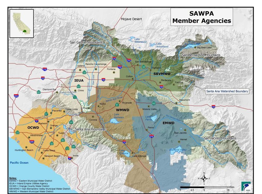
the northwest by the Mojave and San Gabriel watersheds. SAWPA has five
member agencies: Eastern Municipal Water District (EMWD), Inland Empire
Utilities Agency (IEUA), Orange County Water District (OCWD), San
Bernardino Valley Municipal Water District (SBVMWD), and Western
Municipal Water District (WMWD) shown below in Figure 8.
17Greenhouse Gas Emissions Calculator for the Water Sector: Users Manual – California Santa Ana Watershed Basin Study Figure 8: SAWPA member agencies The climate and geography of the State of California present unique challenges to the management and delivery of water. While most of the State’s precipitation falls on the northern portion of the State, the majority of California’s population resides in the semi-arid, southern portion of the State. Water is diverted, stored, and then transferred from the water-rich north to the more arid central and southern sections of the state through the California State Water Project (SWP), the Central Valley Project, and the Los Angeles Aqueduct. In addition to the projects that transport water from the north to the south, the southern coastal area relies on water imported through The Metropolitan Water District of Southern California’s (Metropolitan) Colorado River Aqueduct. The Bureau of Reclamation and seven basin states manage the Colorado River system under the authority of the Secretary of the Interior and for the benefit of the seven basin states. Over-allocation of this resource, along with a U.S Supreme Court Decision (Arizona v. California, 1964) and population and economic growth, led to the recent California “4.4 Plan” and Quantification Settlement Agreement (QSA). The QSA limits California’s share of the Colorado River water supply to 4.4 million acre-feet (MAF). As a result of these actions, Metropolitan’s supply from 18
Greenhouse Gas Emissions Calculator for the Water Sector: Users Manual – California
                                                   Santa Ana Watershed Basin Study

the Colorado River was significantly reduced, especially during extended dry
periods.
In the past, a buffer supply was developed by constructing new facilities, such as
dams and/or aqueducts, to provide water supply for future growth. Today, the gap
between supply and demand has closed and increasing emphasis is placed on
conservation and development of local supplies. Building new facilities is costly
and such projects face strict environmental review before they can be approved.
This has caused California to seek more creative and sustainable solutions to
water resource management.

4.2 Application of the GHG Emissions Calculator to the
SARW
Many factors affect future water demands such as population growth, hydrologic
conditions, public education, and economic conditions, among others. In 1990,
4.2 million people lived in the Watershed. In the 1990s, the population grew by
17.6%, and continued to grow to the present population of approximately 6.1
million, as shown in Figure 9. By 2050, the population is projected to reach 9.9
million (Santa Ana Integrated Watershed Plan, 2002).

Figure 9: Population for the Santa Ana River Watershed

Using the GHG Emissions Calculator, water demand for the SARW was
calculated for the watershed, as a whole, every ten years from 1990-2050, shown
in Figure 10. The population projections from Figure 9 and historic per capita
water use were incorporated to determine the demand (conservation was not taken
into account).

                                                                                  19
Greenhouse Gas Emissions Calculator for the Water Sector: Users Manual – California Santa Ana Watershed Basin Study Figure 10: Santa Ana Watershed water demand calculated for this study The population data found in Figure 9 was used in the GHG Emissions calculator to determine a GHG emissions baseline for the SARW in million metric tons of carbon dioxide equivalent (mtCO2e), shown in Figure 11. Figure 11: Baseline GHG emissions for the SARW 20
Greenhouse Gas Emissions Calculator for the Water Sector: Users Manual – California
Santa Ana Watershed Basin Study
In February 2008, California Governor Schwarzenegger directed state agencies to
develop a plan to reduce statewide per capita urban water use by 20% by the year
2020 (20x2020). The GHG Emissions Calculator was used to evaluate whether
this conservation measure alone would be enough to meet AB 32 targets. The
results, found in Figure 12, show that a 20% reduction by the year 2020 does not
quite allow the SARW to meet the 2020 target (back to 1990 levels). However, if
the SARW reduced per capita water use by 20% and also increased the self-
supplied water by 10% by 2020 through changes to water supply portfolio,
graywater reuse, or rainwater harvesting the AB 32 2020 target could be met, but
the 2050 target of 80% below 1990 levels would not, as shown in Figure 13.
Figure 12: Conservation for SAWR to meet a 20% reduction in GHG
emissions by 2020 (also referred to as 20x2020)
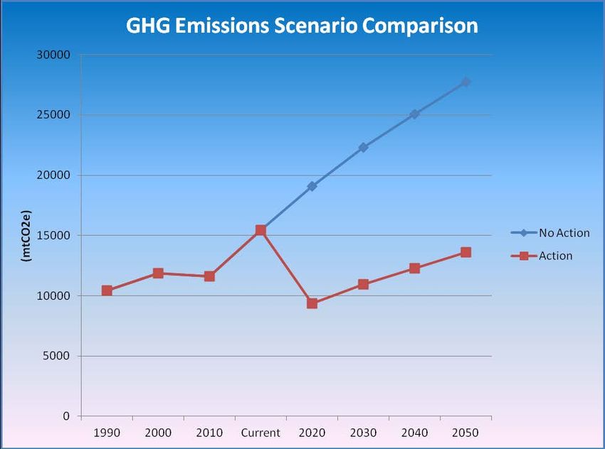
21Greenhouse Gas Emissions Calculator for the Water Sector: Users Manual – California Santa Ana Watershed Basin Study Figure 13: GHG emissions in the SARW resulting from 20x2020 in addition to 10% more self-supplied water by 2020 A 20% reduction in per capita water use every 10 years from 2020 to 2050 in addition to 10% more self supplied water by 2020 was evaluated using the GHG Emissions Calculator. These additional conservation measures only reach 30% below the 1990 GHG emission levels, as shown in Figure 14. One way to reach the AB 32 2050 target of 80% below the 1990 levels of GHG emissions is through a combined conservation per capita water use reduction of 40% each decade (2030-2050) in addition to 20x2020, and in imported water by 10% in 2020 and again in 2030, the results of which are shown in Figure 15. However, this level of conservation may not be feasible for the area. In Figure 16, the three conservation scenarios described above are compared to the no action scenario, a task easily accomplished by the GHG Emissions Calculator. The GHG Emissions Calculator can also be used to evaluate additional measures to reduce GHG emissions including changes to water supply portfolio, graywater reuse, and rainwater harvesting, among many others. It is likely that a combination of measures will be required to meet the GHG emission reduction targets laid out in AB 32. 22
Greenhouse Gas Emissions Calculator for the Water Sector: Users Manual – California
                                                  Santa Ana Watershed Basin Study

Figure 14: GHG emissions in the SARW resulting from a 20% decadal
reduction in addition to 10% more self-supplied water by 2020

Figure 15: SARW GHG emissions resulting from 20x2020 followed by a
40% decadal reduction in GPCD (2030-2050) and decreases in imported
water by 10% by 2020 and 2030

                                                                                 23
Greenhouse Gas Emissions Calculator for the Water Sector: Users Manual – California
Santa Ana Watershed Basin Study
GHG Emissions Scenario Comparison
2000000
1800000
1600000
1400000
1200000
(mtCO2e)
1000000
800000
600000
400000
200000
0
1990 2000 2010 Current 2020 2030 2040 2050
Baseline
20x2020
20x2020 & -10% Imported Water by 2020
20x2020 & -10% Imported Water by 2020 & -40% GPCD Decadally (2030-2050) & additional -10% imported water by 2030
20x2020 & -10% Imported Water by 2020 & -40% GPCD Decadally (2030-2050) & additional -10% imported water by 2030
Figure 16: Comparison of GHG emissions resulting from conservation and
reduced imported water scenarios for the SARW
24You can also read