Hourly surface meltwater routing for a Greenlandic supraglacial catchment across hillslopes and through a dense topological channel network - The ...
←
→
Page content transcription
If your browser does not render page correctly, please read the page content below
The Cryosphere, 15, 2315–2331, 2021
https://doi.org/10.5194/tc-15-2315-2021
© Author(s) 2021. This work is distributed under
the Creative Commons Attribution 4.0 License.

Hourly surface meltwater routing for a Greenlandic supraglacial
catchment across hillslopes and through a dense
topological channel network
Colin J. Gleason1 , Kang Yang2 , Dongmei Feng1 , Laurence C. Smith3,4 , Kai Liu5 , Lincoln H. Pitcher6 , Vena W. Chu7 ,
Matthew G. Cooper8 , Brandon T. Overstreet9 , Asa K. Rennermalm10 , and Jonathan C. Ryan3
1 Department    of Civil and Environmental Engineering, University of Massachusetts Amherst, Amherst, 01002, USA
2 School  of Geographic and Oceanographic Sciences, Nanjing University, Nanjing, 210023, China
3 Institute at Brown for Environment and Society, Brown University, Providence, Rhode Island, 02912, USA
4 Department of Earth, Environmental, and Planetary Sciences, Brown University, Providence, Rhode Island, 02912, USA
5 Nanjing Institute of Geography & Limnology, Chinese Academy of Sciences, Nanjing, 210008, China
6 Cooperative Institute for Research in Environmental Sciences (CIRES), University of Colorado Boulder, Boulder, CO, USA
7 Department of Geography, University of California Santa Barbara, Santa Barbara, 93106, USA
8 Department of Geography, University of California, Los Angeles, Los Angeles, CA, 90095, USA
9 Department of Geology and Geophysics, University of Wyoming, Laramie, WY, 82070, USA
10 Department of Geography, Rutgers, The State University of New Jersey, New Brunswick, NJ 08901, USA

Correspondence: Colin J. Gleason (cjgleason@umass.edu)

Received: 17 September 2020 – Discussion started: 16 October 2020
Revised: 25 February 2021 – Accepted: 26 March 2021 – Published: 18 May 2021

Abstract. Recent work has identified complex perennial           production. We further test hillslope routing and network
supraglacial stream and river networks in areas of the Green-    density controls on channel discharge and conclude that ex-
land Ice Sheet (GrIS) ablation zone. Current surface mass        plicitly including hillslope flow and routing runoff through a
balance (SMB) models appear to overestimate meltwater            realistic fine-channel network (as opposed to excluding hill-
runoff in these networks compared to in-channel measure-         slope flow and using a coarse-channel network) produces
ments of supraglacial discharge. Here, we constrain SMB          the most accurate results. Modeling complex surface water
models using the hillslope river routing model (HRR), a spa-     processes is thus both possible and necessary to accurately
tially explicit flow routing model used in terrestrial hydrol-   simulate the timing and magnitude of supraglacial channel
ogy, in a 63 km2 supraglacial river catchment in southwest       flows, and we highlight a need for additional in situ discharge
Greenland. HRR conserves water mass and momentum and             datasets to better calibrate and apply this method elsewhere
explicitly accounts for hillslope routing (i.e., flow over ice   on the ice sheet.
and/or firn on the GrIS), and we produce hourly flows for
nearly 10 000 channels given inputs of an ice surface digi-
tal elevation model (DEM), a remotely sensed supraglacial
channel network, SMB-modeled runoff, and an in situ dis-         1   Introduction
charge dataset used for calibration. Model calibration yields
a Nash–Sutcliffe efficiency as high as 0.92 and physically re-   The study of supraglacial streams and rivers atop the Green-
alistic parameters. We confirm earlier assertions that SMB       land Ice Sheet (GrIS) is an emerging subfield with implica-
runoff exceeds the conserved mass of water measured in this      tions for the physical understanding of ice sheet subglacial
catchment (by 12 %–59 %) and that large channels do not de-      hydrologic systems, ice motion, and sea level rise (Irvine-
water overnight despite a diurnal shutdown of SMB runoff         Fynn et al., 2011; Rennermalm et al., 2013; Chu, 2014; Flow-
                                                                 ers, 2018; Pitcher and Smith, 2019). When the GrIS surface

Published by Copernicus Publications on behalf of the European Geosciences Union.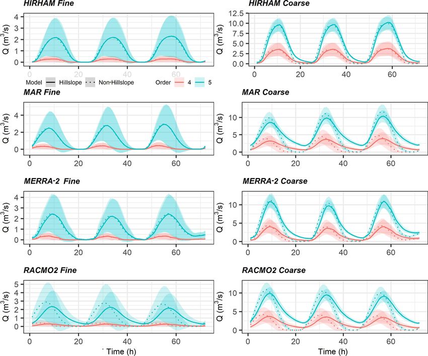
2316                    C. J. Gleason et al.: Hourly surface meltwater routing for a Greenlandic supraglacial catchment

melts, meltwater that is not evaporated, stored, or refrozen      (Banwell et al., 2013, 2016). Leeson et al. (2012) similarly
moves through what is now understood to be a complex              used Manning’s equation to transport water in a 2D grid-
perennial hydrologic system distinct from terrestrial hydrol-     based routing scheme, assigning all grids a uniform Man-
ogy (Yang et al., 2016; Pitcher and Smith, 2019). Recent ad-      ning’s n while not explicitly defining flow differences be-
vances in mapping (Lampkin and VanDerberg, 2014; Rippin           tween flow in channels and flow over bare ice. Liston and
et al., 2015; Smith et al., 2015, 2017; Yang and Smith, 2016),    Mernild (2012) also applied mass conservation at the grid
modeling (Banwell et al., 2012, 2016; Clason et al., 2015;        cell level to route runoff between grid cells and did not ac-
Karlstrom and Yang, 2016; Yang et al., 2018) and measuring        count for the presence of channels that convey this runoff
(McGrath et al., 2011; Legleiter et al., 2014; Gleason et al.,    with distinct hydraulics. Smith et al. (2017) attempted to
2016; Smith et al., 2017) supraglacial channel networks have      address this channel routing via the classic empirical Sny-
revealed numerous similarities to terrestrial watersheds, but     der synthetic unit hydrograph (SUH) model (Snyder, 1938)
their scale and remoteness have limited the number of field       to calculate discharge hydrographs for the terminal moulins
studies.                                                          of 799 internally drained surface catchments in the south-
   This new appreciation for supraglacial hydrologic pro-         west GrIS. Yang et al. (2018) used a similar classic empir-
cesses has emerged at a time of increasing accuracy and           ical model, the rescaled width function (RWF; Rinaldo et
sophistication of surface mass balance (SMB) modeling of          al., 1995), to partition the ice surface into slow-flowing inter-
the GrIS. SMB models use regional atmospheric forcing to          fluvial (i.e., hillslope) and fast-flowing (open-channel) zones
simulate GrIS surface mass balance components, including          and calculated moulin discharge while improving the physi-
the amounts of meltwater production and of liquid water in        cal realism of the supraglacial routing process. Importantly,
excess of evaporation and retention and refreezing (termed        Yang et al. (2020) demonstrated the likelihood of subsur-
“runoff”) available for hydrologic functions (Fettweis et al.,    face unsaturated zone flow even through bare glacial ice, a
2020; Vernon et al., 2013). SMB models here refer to any          phenomenon confirmed by field (Cooper et al., 2018; Irvine-
global and/or regional circulation model (G/RCM) or reanal-       Fynn et al., 2011; Munro, 2011) and theoretical (Karlstrom
ysis that explicitly simulates ice sheet surface runoff. These    and Yang, 2016) studies. Yang et al. (2020) recently com-
models are grid-based and operate at pan-GrIS scales, pro-        pared several of these empirical models and found they in-
ducing a single runoff value for a given model grid and time      troduce significant variability in diurnal moulin discharges
step. Note that the terrestrial hydrology community com-          and corresponding subglacial effective pressures.
monly uses the term “water excess” to represent the vol-             These previous efforts demonstrated successful meltwater
ume of water available for routing after hydrologic processes,    transport modeling on the GrIS ablation zone and its neces-
while the glaciology community uses the term “runoff” to          sity, but their relative simplicity allows space for the applica-
represent this same quantity specific to ice sheets. Most ex-     tion of sophisticated routing models from terrestrial hydrol-
isting SMB models do not route this runoff and instead as-        ogy to be applied to ice sheet surfaces more generally. For
sume that all runoff not refrozen in snow or firn leaves the      instance, Lin et al. (2019) used gridded estimates of water
ice sheet as soon as it is produced (Fettweis et al., 2020).      excess (analogous to runoff) to simulate daily flows in nearly
In reality, observations of the GrIS surface indicate that lake   three million river reaches between 1979 and 2013 with fully
impoundment (e.g., Arnold et al., 2014), flow through weath-      conserved mass and momentum in realistic river networks
ering crust (e.g., Cooper et al., 2018), and transport through    globally. This undertaking was the first demonstration of this
supraglacial stream and river networks modify the timing and      capability at global scale following years of well-established
magnitude of excess water reaching moulins or the ice sheet       theoretical work and advances in hydrologic representation
edge (Smith et al., 2017). Modeling these processes is pre-       for big data. This routing approach is suitable for represent-
cisely analogous to the use of land surface models in terres-     ing GrIS surface water transport processes as gridded runoff
trial hydrology, whereby a land surface model (SMB model          on ice sheets must be routed through supraglacial rivers,
here) produces gridded water excess (runoff here) and then        lakes, and hillslopes (which include firn atop the GrIS), as on
routes this water with a coupled routing model. Coupling sur-     land. Building and calibrating models to route water through
face water processes to SMB models, loosely or tightly, is        landscapes and channel networks while obeying fundamental
thus needed for a fuller representation of GrIS supraglacial      principles of mass and momentum conservation is an estab-
hydrology to align this field with practices in terrestrial hy-   lished practice in terrestrial hydrology that may readily be
drology (e.g. Bates et al., 1997; Beighley et al., 2009; Wood     applied to ice sheet surfaces as well.
et al., 2011; Lin et al., 2019).                                     There are several barriers to applying such routing for the
   Previous studies have begun to stich these two research        GrIS at the catchment scale. First, routing models require a
avenues together. For example, Banwell et al. (2012) used         well-defined channel network with explicit and continuous
Darcy’s law to describe meltwater flow routing through snow       topology. There have been demonstrations of network map-
and Manning’s equation to describe lateral runoff transport       ping (Yang et al., 2016) and topology generation (King et al.,
across bare ice and then later used this meltwater to fill        2016), but to our knowledge no automated, large-network-
supraglacial lakes or supply surface meltwater to moulins         scale (i.e., catchments with thousands of channels or more)

The Cryosphere, 15, 2315–2331, 2021                                                   https://doi.org/10.5194/tc-15-2315-2021
C. J. Gleason et al.: Hourly surface meltwater routing for a Greenlandic supraglacial catchment                                2317

coupled extraction and topological connection work exists           perennial and well-drained supraglacial stream and river
for the GrIS. Existing terrestrial routing models like the hill-    network during peak flow periods of late summer. Smith
slope river routing model (HRR; Beighley et al., 2009) stand        et al. (2017) report that the basin elevation spanned ap-
ready to route runoff “off the shelf”, yet these cannot be ap-      proximately 1200–1400 m in 2015, with air temperatures
plied until a generalizable automated extraction and topo-          in the summer measurement period ranging from −3 to
logical connection process is available. Applying a model           2 ◦ C and net radiation ranging from approximately −100 to
such as HRR could also further understanding of GrIS river          300 W/m2 . Previous work in the basin includes (i) a compari-
networks, which is currently underdeveloped (Pitcher and            son of SMB runoff and field-measured discharge using a sim-
Smith, 2019). For instance, the relative importance of hill-        pler routing method (Smith et al., 2017), (ii) a study of sub-
slope flows and channel density on runoff transport have not        surface water storage in bare-ice weathering crust (Cooper et
been explored on a first-principles basis at network scales,        al., 2018), (iii) albedo mapping (Ryan et al., 2017), and (iv)
and model parameters controlling hillslope friction, channel        satellite and uncrewed aerial vehicle (UAV) remote sensing
friction, and runoff reduction and augmentation could reveal        work to map the catchment’s supraglacial channel network
how these physical processes interact to produce channel dis-       (Ryan et al., 2017; Yang et al., 2018). Readers are referred to
charges.                                                            these published works for more information on the physical
   In this paper we use HRR to advance the physical un-             setting of the basin. Here we use the Rio Behar specifically
derstanding of GrIS supraglacial meltwater transport pro-           because it is the only known large GrIS supraglacial river
cesses as follows. (1) We automatically generate spatially          catchment with an hourly in situ record of channel discharge
explicit topological networks of varying drainage densities         (see Sect. 2.2). Other discharge records exist, as, for instance,
for a supraglacial catchment for which a brief (72 h) in            McGrath et al. (2011) who provide hourly discharge records
situ record of outlet channel discharge is available. (2) We        for a small (1.1 km2 ) catchment, while Chandler et al. (2013)
route water runoff generated by four different SMB models           give hourly moulin (fed by a channel) discharge for another
through these networks at an hourly timescale. (3) We con-          small catchment, but the size of Rio Behar and the wealth of
strain and calibrate the routing via hourly in situ discharge       previous work therein makes it an ideal setting for this study.
measurements and previously published field measurements            Using high-resolution remote sensing, the watershed is delin-
of supraglacial channel frictions and velocities. Our initial       eated to an in situ streamflow measurement point (Sect. 2.2)
routing results immediately revealed a mismatch between             that defines the outlet located less than 1 km upstream of the
modeled and routed runoff and measured channel flows, so            catchment’s terminal moulin. Because all meltwater runoff
our philosophy for this study is to assume that measured dis-       passing out of our watershed penetrates the ice sheet via a
charge at the outlet is correct and calibrate SMB runoff vol-       moulin, accurate modeling of this water flux is important for
umes and channel properties to match discharge observations         studies of GrIS subglacial hydrology and ice dynamics (Chu,
as mediated through the physics of the routing model. (4)           2014; de Fleurian et al., 2016; Banwell et al., 2016; Flowers,
To advance understanding of hillslope processes and chan-           2018; Davison et al., 2019)
nel density on meltwater transport, we design an experiment
to test how the representation of hillslope processes and net-      2.1   Remotely sensed and SMB model data
work density (as derived by our automated network genera-
tion process) affects the routing model. We ultimately route        A high-resolution remotely sensed supraglacial stream net-
meltwater through thousands of supraglacial channels every          work for the Rio Behar catchment, mapped from a 0.5 m res-
hour, and we solve (via conservation of mass and momentum           olution panchromatic WorldView-2 satellite image acquired
inherent to routing) for the roles of channel friction, hillslope   on 18 July 2015, was obtained from Smith et al. (2017), and
delay, and network density in controlling the magnitude and         this scale is sufficient for capturing the smallest streams in
timing of water fluxes through supraglacial channels and ul-        this region (Yang et al., 2018). The stream network prod-
timately moulin injection in our test watershed. These proce-       uct of Smith et al. (2017) was combined with a seasonally
dures and results form a blueprint for the general coupling of      simultaneous portion of the 2 m resolution ArcticDEM digi-
runoff modeling, water transport, and channel processes atop        tal elevation model (DEM) obtained from the Polar Geospa-
the GrIS.                                                           tial Center (Porter et al., 2018) to produce two distinct
                                                                    supraglacial stream networks, as described in Sect. 3.2. The
                                                                    ArcticDEM has been widely used in GrIS hydrology studies
2   Study area and data                                             and performed reasonably well in representing drainage pat-
                                                                    terns in previous work (e.g., Moussavi et al., 2016; Pope et
We develop our routing model for Rio Behar, a previously            al. 2016; Yang et al., 2020).
studied, internally drained supraglacial river catchment in            GrIS runoff was simulated by four models (HIRHAM5,
southwest Greenland. First introduced by Smith et al. (2017),       MAR3.6, RACMO2.3, and MERRA-2). Data and detailed
the Rio Behar catchment is approximately 63 km2 and cen-            descriptions of these SMB models are provided in Smith et
tered at 67.04◦ N and 48.55◦ W with a highly developed              al. (2017), but in brief each of these models solves a local

https://doi.org/10.5194/tc-15-2315-2021                                                   The Cryosphere, 15, 2315–2331, 2021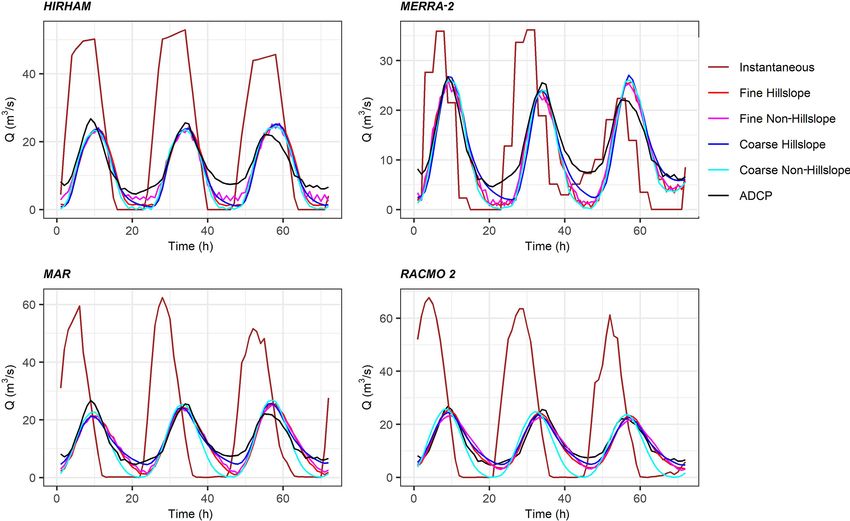
2318                     C. J. Gleason et al.: Hourly surface meltwater routing for a Greenlandic supraglacial catchment

surface energy balance from meteorological forcing to pro-          using traditional surveying, radar velocimetry, and an ADCP.
duce some amount of runoff produced after physical pro-             These measurements in turn yielded derivative estimates of
cesses of melting, condensation, retention, and refreezing.         discharge, stream power, Froude number (a classic index of
This excess water is spatially gridded, and for a given grid        flow velocity in open-channel hydraulics), and roughness co-
cell the models each produce hourly runoff, which we as-            efficient (Manning’s n) at 64 sites, representing the largest
sume is topographically constrained and transported exclu-          known empirical dataset of supraglacial channel hydraulic
sively via surface/near-surface transport. We take the average      properties currently available in the literature. Site locations
runoff in all grid cells intersecting Rio Behar (ranging from       ranged from 502 to 1485 m elevation and up to 74 km inland
one to eight SMB grid cells for the four models) to arrive at       from the ice margin, and instantaneous discharges ranged
a single hourly runoff value for each SMB model following           from 0.006 to 23.12 m3 /s in actively flowing channels 0.20
Smith et al. (2017). We therefore have four different runoff        to 20.62 m wide. These observations are used to constrain
forcings available for routing that cover from 1 month be-          our modeled roughness coefficients to produce realistic pa-
fore the in situ measurement period through the end of the          rameters and velocities. Section 3.3 describes this process
measurements (Sect. 2.2). Our goal for this paper is not to         fully. Note that we cannot use these observations to validate
interrogate these models. Rather, we hope to highlight the          our routing model and instead use them to inform it. These
nuances of supraglacial meltwater routing across a range of         point measurements could in theory be reproduced by our
forcings.                                                           hydraulic model, but to do so would require measurements
                                                                    of channel properties and runoff upstream of each point for
2.2    In situ data                                                 several hours/days before each hydraulic measurement was
                                                                    taken, and such data do not exist.
Two sources of field data are available for this study. The first
source is an hourly acoustic Doppler current profiler (ADCP)
discharge record published by Smith et al. (2017). An ADCP          3     Methods
is an instrument that measures river flow depth via sonar
ranging and vertical velocity profiles using Doppler shifts in      3.1    Experiment design
the water column. The instrument is transited orthogonal to
flow and makes its measurements in discrete bins which are          Our overall goal for this study is to improve the current
then summed to arrive at the mass flux of water in the chan-        understanding of supraglacial hydrological transport pro-
nel. ADCP outputs are thus correctly labeled as “estimates”         cesses by classically modeling hillslope and channel rout-
of discharge rather than “measurements” as the measured             ing. We test two experimental settings (inclusion/exclusion
quantities are depth and velocity and discharge is derived.         of hillslope flow, coarse-/fine-channel network densities) on
However, the ADCP provides the most trusted and accurate            four different SMB models to produce 16 experimental runs
method for estimating discharge used in hydrology, and its          (4 runs per model; Fig. 1). These runs are labeled as either
discharge estimates are frequently labeled as measurements          “fine” or “coarse” and “hillslope” or “non-hillslope”; so, for
(Gleason and Durand, 2020). Further reading on ADCP esti-           example, an experiment using a fine-network density and ex-
mates of discharge and measurement protocols can be found           cluding hillslope processes would be labeled “non-hillslope
in Turnipseed and Sauer (2010).                                     fine.” For each run, we calibrate 11 parameters: a global
   Smith et al. (2017) obtained hourly measurements of dis-         runoff correction coefficient (1 parameter), a spatially ex-
charge via ADCP at the outlet of Rio Behar from 13:00 UTC           plicit channel roughness coefficient binned by channel slope
on 20 July 2015 to 12:00 UTC on 23 July 2015. Smith et              (9 parameters), and a global hillslope roughness coefficient
al. (2017) give a detailed description of measurement pro-          (1 parameter) to optimize modeled and measured discharge
tocol for collecting and processing these ADCP discharges,          at the basin outlet (Sect. 3.3.2 gives full details). Model cal-
and readers are referred to that publication for more in-           ibration statistics were used as indicators of the physical re-
formation. ADCP estimated discharges ranged from 4 to               alism of each experiment, and we seek to identify robust,
26 m3 /s, revealing that large supraglacial rivers do not de-       cross-SMB model parameter trends in our factorial experi-
water at night and can sustain peak flows comparable to             mental setting. Thus, we calibrate HRR 16 separate times to
streams of moderate catchment size in terrestrial hydrology.        produce a set of results that vary by runoff forcing, channel
These ADCP discharges form the core HRR model calibra-              density, and inclusion/exclusion of hillslope process.
tion dataset for our study.                                            Note that in all configurations (Fig. 1), we calibrate a
   The second source of in situ data used here is a broad set       runoff correction coefficient (Rcoef ). Previous work compar-
of observations of supraglacial channel hydraulics collected        ing SMB runoff to ADCP discharge at our field site reveals
in summer 2012 across 64 supraglacial streams and rivers of         that the SMB runoff is frequently greater than observed dis-
the southwest GrIS (Gleason et al., 2016). These in situ mea-       charge leaving the watershed (Smith et al., 2017). We there-
surements consist of instantaneous supraglacial channel flow        fore created a multiplicative runoff correction coefficient
widths, depths, water surface slopes, and velocities collected      to either reduce or augment SMB runoff that is calibrated

The Cryosphere, 15, 2315–2331, 2021                                                    https://doi.org/10.5194/tc-15-2315-2021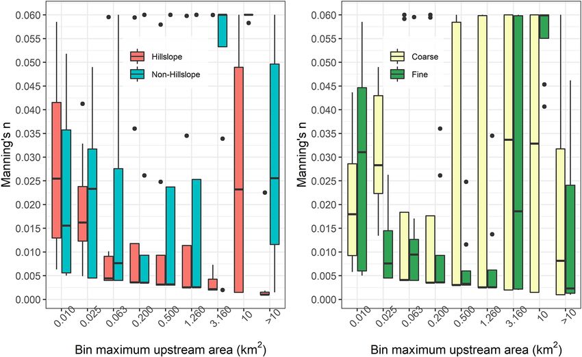
C. J. Gleason et al.: Hourly surface meltwater routing for a Greenlandic supraglacial catchment                              2319

within HRR without changing the timing of production. Pre-         Since we know that a river or stream channel is abruptly
vious routing studies have forced model runoff to equal the        deeper than its surrounding banks, artificially lowering ele-
cumulative measured river discharge before further routing         vations where we observe channels ensures that these loca-
(Smith et al., 2017), yet this restrictive assumption amounts      tions are the lowest feature in the surrounding terrain and
to an empirical ad hoc mass conservation rather than explic-       therefore collect topographically driven water. In DEM pro-
itly relying on hillslope and channel mass and momentum            cessing for hydrology, a depression is an area where water
conservation across thousands of channels. Thus, we cali-          pools as the flow direction is always downhill as in the sides
brate Rcoef , together with the traditional HRR parameters         of a bowl. These depressions typically need to be artificially
(i.e., channel and hillslope roughness coefficients; Table 1;      “filled”, that is, their elevations need to be raised, as other-
Sect. 3.3.2), for each model run to learn the total volume of      wise the topography indicates that water cannot leave once
excess needed in each case to simultaneously match both hy-        it enters the depression. Because we “burn in” stream loca-
drograph timing and mass conservation. This allows our re-         tions to the DEM, standard sink filling is not required for this
sults and routing framework to guide our conclusions on the        analysis (we lower streams rather than raise depressions),
total volume of water needed to generate the outlet hydro-         but two large topographic depressions in the DEM of our
graph as this volume might differ between network and hill-        catchment required further processing even after burning in
slope configurations. Further, the use of a single Rcoef allows    streams. Standard DEM preparation for network generation
us to accurately model discharge without allowing the attri-       dictates that upstream depressions are filled, while outlet de-
bution of errors in runoff production: these could stem from       pressions are preserved, yet this assumption generated unre-
SMB errors, unaccounted for refreezing, storage, or lake fill-     alistic parallel drainage channels upstream and no channels
ing, surface transport that violates topographic constraints,      in the outlet depression for our data. To address this problem,
englacial draining, or ADCP measurement error. Our frame-          (2) a priority-flood algorithm (Lindsay, 2016) was applied to
work is unable to apportion any gaps in runoff production and      breach the two depressions and to create a continuously flow-
routed discharge to any of these sources, and thus our treat-      ing, realistic drainage network for the catchment (Fig. 2). Fi-
ment of runoff as a bulk reduction/augmentation is faithful to     nally, (3) the parameter that drives network generation and
our experiment design and article goals.                           ultimately channel density is the channel initiation threshold:
                                                                   the minimum area needed to form a free-flowing channel.
3.2   River network extraction                                     This concept stems from the fact that above river headwa-
                                                                   ters, water simply flows through the soil and not on the sur-
Although Smith et al. (2017) provide a topologically con-          face until the water table elevation exceeds the soil elevation
nected channel network for our study area (i.e., they explic-      in a spring. We observe an exact analogue on the GrIS: chan-
itly defined how every channel is connected to every other         nels dwindle in size until they become indistinguishable from
channel throughout the entire network to allow water to flow       wet firn and/or ice near topographic divides (Gleason et al.,
from the headwaters to the outlet to obey observed channel         2016). To estimate the impact of drainage patterns on melt-
connections), we are interested in generalizing the process        water routing, we tested both a large (104 m2 ) and a small
of water routing in cases when preexisting channel network         (103 m2 ) channel initiation threshold to create a “coarse” and
maps do not exist. Further, we must generate different river       a “fine” supraglacial drainage network, respectively, from the
networks to test the effects of network density on the routing     DEM (Fig. 2). These two modeled stream networks both fol-
model. Therefore, we introduce a process to create models of       low the channel map from Smith et al. (2017), with the key
complete river networks as defined by topography that can in       difference that the coarse network does not produce the nar-
theory be applied to any area of the GrIS with a high-quality      rowest streams we know to exist. This enabled us to test the
DEM and a remotely sensed image. This topographically de-          effects of including or excluding very small tributary streams
fined flow is a classic practice in terrestrial hydrology, and     on surface water routing. We assign channel widths to each
since all open-channel flow is gravity-driven, this practice ap-   DEM-derived channel from the channel map of Smith et
plies for flow routing through any medium without substan-         al. (2017), and since the DEM process begins with burning
tial pressure forces. Topographically defined flow has there-      in these streams, there is always a 1 : 1 assignment of chan-
fore been applied/invoked for a variety of surfaces, including     nel width from imagery to network model. Our fine-channel
Mars (e.g., Dohm et al., 2001; Rodriguez et al., 2005; Fassett     network produces streams with a minimum width of 0.5 m,
and Head, 2008)                                                    matching to the correct order of magnitude the reporting by
   To generate our river networks, (1) we first “burned” (i.e.,    Gleason et al. (2016) of channels as narrow as 0.2 m. The
lowered the pixel elevations) the remotely sensed stream map       coarse network produced streams with a minimum width of
of Smith et al. (2017) into ArcticDEM, a standard hydro-           0.7 m, suggesting it is excluding the smallest streams in the
logic practice (e.g., Lindsay, 2016). This process ensures that    remotely sensed map. GrIS supraglacial channels incise and
channels are lower than surrounding topography as remotely         meander over time, yet HRR cannot represent this behavior
sensed DEMs cannot “see” channel bottoms and therefore             and instead assumes that channels remain fixed in space and
create smooth surfaces where surface water features exist.         time. It would be possible to derive expected erosion and in-

https://doi.org/10.5194/tc-15-2315-2021                                                 The Cryosphere, 15, 2315–2331, 2021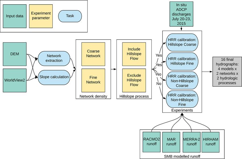
2320 C. J. Gleason et al.: Hourly surface meltwater routing for a Greenlandic supraglacial catchment
Figure 1. Schematic diagram of our experimental design and modeling procedure. Hillslope river routing (HRR) model inputs, processes, and
outputs are labeled. This workflow yields 16 independent hydrographs by considering fine vs. coarse supraglacial channel network densities
and inclusion vs. exclusion of hillslopes in addition to open-channel flow.
cision (and additional meltwater) due to frictional heating of ble in the coarse network, and lakes connected to the channel
the channels, but without including a radiation budget and ice network (i.e., have an inflow and outflow) are represented by
property data we could not model how the stream network wide, shallow “throughflow” river segments as all are non-
changes in time nor satisfactorily model this additional melt- terminal with outflow channels. Lakes on the GrIS evolve
water with commensurate sophistication to the SMB runoff seasonally; they begin pooling water in the early melt sea-
forcing (i.e., tight coupling with SMB models). Instead, we son until an outlet elevation is reached, and then they begin
model these network snapshots with HRR loosely coupled to spill downstream. Our data come from peak melt season
with SMB runoff (as opposed to tightly coupled, when SMB when lakes are full, and thus any lake connected to the net-
runoff would be an input into network generation), which is work will behave fluvially, that is, it will spill according to
reasonable for our 1-month experiment (Sect. 3.3.1). its slope, volume, and lateral input via the conservation of
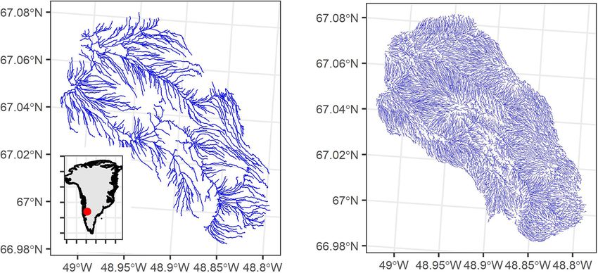
Our river network extraction produced two topologically mass and momentum. Further, Fig. 2 indicates that there are
connected networks of 1044 and 8095 channels (coarse and likely no lakes in the watershed that are disconnected from
fine, respectively; Fig. 2). The coarse network has six stream the channel network – our drainage density is sufficient to
orders (the smallest streams on the landscape are defined as ensure that lakes of any appreciable size would be captured
order 1, and every junction of stream produces a new stream as a throughflow segment.
of higher order) and the fine network seven orders. Stream
orders are a shorthand for the hydraulic complexity of a net- 3.3 River routing
work as the number and length of streams in a given order
both increase geometrically (Horton, 1945). Therefore, our 3.3.1 Model setup
finding of almost an order of magnitude more channels in
HRR routes water excess over the land surface and through
the fine seven-order network than the course six-order net-
channels. In channels, it follows the Muskingum–Cunge
work matches theory. The networks are topologically com-
equation, a kinematic wave approximation of the 1D St.
plete (i.e., all channels are explicitly connected to one an-
Venant equations (conservation of mass and momentum in
other and preserve their hydrologic hierarchy), allowing for
an open channel; Cunge, 1969). HRR uses an explicit kine-
successful routing without the need for further correction of
matic wave for hillslope transport as non-channelized over-
network connections. The main trunk streams only are visi-
land flow (Li et al., 1975). HRR requires inputs of channel
The Cryosphere, 15, 2315–2331, 2021 https://doi.org/10.5194/tc-15-2315-2021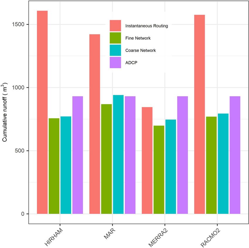
C. J. Gleason et al.: Hourly surface meltwater routing for a Greenlandic supraglacial catchment                                    2321

Figure 2. The 1044 segment “coarse” network and the 8095 segment “fine” network were automatically extracted from a DEM and remotely
sensed data. These river networks represent different channelization area thresholds, and test how assumptions of network density control
hydrologic process.

widths and lengths, which are assumed to be invariant and              so we calibrate our routing model to outlet discharges de-
derived from remote sensing (Sect. 2.1), channel slope, and            spite producing discharges in thousands of reaches. A very
each channel’s subcatchment area and total upstream area, as           large amount of literature on hydrologic model optimization
derived here from the DEM, in which bed slope is assumed to            and calibration exists, and interested readers are referred to
equal the free surface flow, consistent with Manning’s equa-           Kirchner (2006) and Gupta et al. (1998) for broad overviews
tion. In addition, the network topology derived in Sect. 3.2 is        of the subject. We perform calibration using an established
required so that HRR can conserve mass and momentum in a               evolutionary algorithm (EA; NSGA II; Deb et al., 2002) as
downstream direction and across channel junctions. HRR is              EAs are efficient estimators in large parameter spaces that
one of several routing models that classically conserve mass           can achieve near-optimal results (Gleason and Smith, 2014).
and momentum designed for large-network applications. Our              This calibration ensures a heuristically optimized outlet hy-
choice of HRR is based on familiarity, model speed (written            drograph but does not explicitly calibrate upstream reaches.
in FORTRAN and called from the RStudio software package                However, since outlet flows are the sum effect of the routing
here), and its rigorous representation of network routing and          delays and volumes of all upstream reaches, and since we ex-
classic open-channel flow hydraulics.                                  plicitly conserve mass and momentum, a well-calibrated out-
   HRR routes time-varying runoff onto existing flows, com-            let should satisfactorily model upstream flows, but we cannot
monly onto a baseflow in terrestrial hydrology. We “spin up”           validate these upstream reaches. Therefore, we constrain al-
the model by routing a constant forcing of median observed             lowable parameters in upstream reaches (and therefore their
ADCP flow through the model rather than attempt to define              discharges and velocities) using the in situ observations of
a minimum baseflow. This steady forcing allows all channels            Gleason et al. (2016).
to fill with water and accurately transfer runoff from the SMB            We calibrate 11 constrained parameters (Table 1) which
models through the system. We used a 3-month spin-up pe-               represent three physical concepts: channel friction (here ex-
riod then temporally varied flows beginning on 1 July from             pressed as Manning’s n and binned by upstream area into
SMB forcing. Our experiment begins on 20 July, and thus                9 separate parameters), hillslope friction, and a water ex-
the model has time to adjust to runoff forcing and mitigate            cess adjustment coefficient. Channel friction is represented
the impact of this spin-up flow before we begin to validate            by Manning’s n, and the EA solves for a single n per bin
the model.                                                             and assigns that n to all streams falling within that drainage
                                                                       area threshold. Manning (1891) generalized open-channel
3.3.2   Model calibration                                              flow into a simple equation in which all flow resistances are
                                                                       lumped into a single empirical parameter n, and over a cen-
Nearly all hydrologic models require calibration to func-              tury of subsequent research has related n to landscape vari-
tion well. To calibrate terrestrial routing models, hydrolo-           ables, channel form, and other geomorphic controls. Our bin-
gists typically iterate parameters until hydrographs at one            ning of Manning’s n follows general hydraulic correlations
or more reaches match a stream gauge in that reach. Here,              between channel size, slope, total discharge, and n (Brinker-
we have calibration data available only at the basin outlet,

https://doi.org/10.5194/tc-15-2315-2021                                                      The Cryosphere, 15, 2315–2331, 2021
2322 C. J. Gleason et al.: Hourly surface meltwater routing for a Greenlandic supraglacial catchment Figure 3. The hourly in situ ADCP hydrograph at the basin outlet (in black) clearly shows the necessity of delaying and reducing SMB modeled runoff (“instantaneous”, brown lines) to match field observations. Even after coupling SMB models with HRR routing models, most simulations underpredict low flows. Peak flows are relatively well modeled, although ADCP peak recession is only modeled correctly by RACMO2-forced routing. hoff et al., 2019). Hillslope flow is modeled as an explicit friction in tandem with runoff production to best match the kinematic wave for non-channelized flow (Li et al., 1975), ADCP record measured at the outlet. Recall we do not run which requires a surface roughness coefficient (i.e., hillslope the SMB models directly. friction), and we limit hillslope friction to between 0.05 (non- We parameterized our EA as follows. Crossover probabil- dimensional; a hillslope with friction equivalent to a rough ity and distance were set to 0.7 and 5, respectively, and muta- channel) and 25 (a hillslope with extreme friction to approx- tion probability and distance were set to 0.2 and 10, respec- imate slow interflow through weathering crust). For context tively. These parameters control the degree of change in one from the terrestrial hydrology literature, McCuen (2004) pro- parameter set to the next. The objective function for the EA vides a reference table for watershed surface roughness with was the Nash–Sutcliffe efficiency (NSE) at the outlet, calcu- hillslope friction values ranging from 0.01 to 0.8. Kalyanapu lated between the in situ ADCP record and the model dis- et al. (2010) developed another reference table based on the charge. NSE is a standard hydrology metric for hydrograph National Land Cover Database, and their values range be- analysis which is optimal at a value of 1. An NSE of 0 is tween 0.01 and 0.4, while Hergarten and Neugebauer (1997) equivalent to modeling a hydrograph as the true mean flow, suggest friction up to a value of 1. Thus, we allow GrIS ice and negative NSE values indicate that the mean outperforms surface hillslope frictions to vary up to 2 orders of magnitude a given model. Finally, we set the population size and num- greater than typical terrestrial reference values to allow for ber of generations (parameters that control how many dif- potentially unique supraglacial processes ranging from fast ferent solutions the EA tests, in tandem with crossover and flow over smooth bare ice to slow porous-media flow through mutation) based on the model configuration (e.g., fine net- weathering crust. Finally, we bound Rcoef to range between works with hillslope processing take much longer to run and 0.3 and 2.0 to allow for both the over- and underproduction therefore used less generations; see below) due to runtime. of water excess without imposing mass (e.g., runoff) pro- Even though we ran our tests using parallel computing on duction. For each of our 16 experimental trials, the EA thus a powerful modeling machine (Intel Xeon Gold 6126 3 GHZ solves for the optimal combination of hillslope and channel CPU with 96 GB of RAM and 24 logical processors), a single The Cryosphere, 15, 2315–2331, 2021 https://doi.org/10.5194/tc-15-2315-2021
C. J. Gleason et al.: Hourly surface meltwater routing for a Greenlandic supraglacial catchment                                   2323

Table 1. Field-based constraints on HRR routing model parameters        bration statistics show high skill (defined here as NSE >0.8)
(from the literature and Gleason et al., 2016).                         in 5 of the 16 cases and moderate skill (NSE >0.5) in all
                                                                        16 cases, with RMSE ranging from 1.85 to 4.55 m3 /s (ob-
        Parameter              Min      Max    Upstream area (km2 )     served flows ranged from 4.6 to 26.7 m3 /s, for context). Note
        Hillslope              0.05      25    n/a (global parameter)   that RMSE and NSE do not track perfectly given the differ-
        friction                                                        ing nature of their assessments. RMSE is a total mass error
                                                                        that is influenced by the scale of variation in the hydrograph,
        Rcoef                   0.3      2.0   n/a (global parameter)   while NSE compares to the mean. There is no universally ac-
        n1                   0.0050   0.0600   area
2324 C. J. Gleason et al.: Hourly surface meltwater routing for a Greenlandic supraglacial catchment
Table 2. Calibrated parameters for all 16 coupled SMB–HRR model experiments. Table is ranked by NSE per row, with the top performing
model in the first row.
Experimental setup Calibrated model parameters Performance metrics
SMB Hillslope Network Rcoef n nSD Hillslope NSE KGE RMSE
forcing density friction (m3 /s)
RACMO2 Included Coarse 0.50 0.027 0.026 13.64 0.92 0.96 1.85
RACMO2 Included Fine 0.49 0.008 0.014 25.00 0.89 0.87 2.17
MAR Included Coarse 0.66 0.011 0.017 14.34 0.89 0.94 2.19
RACMO2 Excluded Fine 0.50 0.015 0.022 – 0.86 0.92 2.49
MAR Excluded Fine 0.63 0.019 0.025 – 0.80 0.83 2.96
HIRHAM Excluded Fine 0.47 0.026 0.019 – 0.79 0.77 3.03
MERRA2 Excluded Fine 0.84 0.021 0.024 – 0.76 0.71 3.20
MERRA2 Included Coarse 0.88 0.006 0.007 5.44 0.75 0.73 3.31
MAR Included Fine 0.61 0.016 0.019 0.05 0.74 0.75 3.35
MERRA2 Included Fine 0.82 0.016 0.019 0.05 0.71 0.75 3.51
MERRA2 Excluded Coarse 0.80 0.025 0.024 – 0.64 0.59 3.95
HIRHAM Included Coarse 0.48 0.006 0.007 1.78 0.62 0.63 4.03
MAR Excluded Coarse 0.55 0.044 0.025 – 0.60 0.57 4.15
HIRHAM Included Fine 0.47 0.031 0.021 0.05 0.57 0.60 4.30
HIRHAM Excluded Coarse 0.46 0.022 0.026 – 0.56 0.56 4.37
RACMO2 Excluded Coarse 0.41 0.055 0.012 – 0.52 0.59 4.55
4.2 Lower-order hydrographs
While we cannot verify flows at any network channel besides
the outlet, we have simulated hourly flows for all 1044 and
8095 channel segments in the coarse and fine networks, re-
spectively. If we assume that accurate model performance at
the main basin outlet indicates physically realistic upstream
flows, it is profitable to report results for upstream flows dur-
ing the calibration period. To analyze these large datasets, we
summarize flows in the 72 h validation period by stream or-
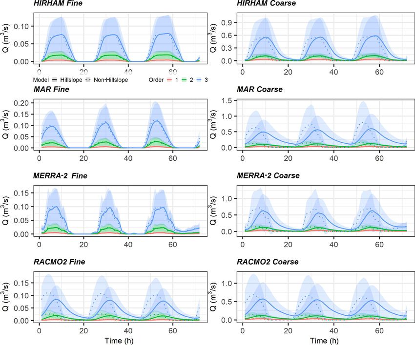
der, with Fig. 5 presenting results for 1st–3rd order streams
and Fig. 6 presenting results for 4th and 5th order streams.
In each figure, we plot the mean hydrograph for the order
with 1-standard-deviation shaded area to represent variabil-
ity around the mean. Geomorphic theory predicts a geomet-
ric decline in the number of streams per order (Allen et al.,
2018), and thus orders with fewer streams are more homoge-
nous by definition in these plots.
There is a large difference in flow magnitude across fine
and coarse models regardless of SMB forcing or inclu-
sion/exclusion of hillslopes (Figs. 5, 6). For 4th and 5th or- Figure 4. Total cumulative discharge for hillslope-enabled scenar-
der streams these flow differences span roughly a factor of 2, ios for the 72 h ADCP measurement period. Total water export is
while in the lower orders flow differences span almost an or- relatively consistent across all four SMB models but substantially
der of magnitude. This signifies that smaller streams are more different than input runoff (i.e., instantaneous routing) for all mod-
els but MERRA2. The ADCP represents a measured cumulative ex-
sensitive to their hillslopes, as expected. We also note that the
port, while instantaneous routing assumes that SMB runoff immedi-
networks have different total orders (six for the coarse net- ately leaves the watershed as soon as it is produced. Calibrated mod-
work, seven for the fine network). Therefore, the 2nd order els underpredict water export due to the underestimation of night-
fine streams loosely correspond to 1st order coarse streams, time low flows.
but this correlation is not a 1 : 1 match. Peak timing also dif-
fers between hillslope and non-hillslope models in the lower
orders for coarse networks. This effect is more pronounced
The Cryosphere, 15, 2315–2331, 2021 https://doi.org/10.5194/tc-15-2315-2021C. J. Gleason et al.: Hourly surface meltwater routing for a Greenlandic supraglacial catchment 2325
Figure 5. Mean and 1-sigma shaded variability for channel segment hydrographs by order for 1st–3rd order streams for the validation period.
Non-hillslope process flows are dashed. Note the increase by a factor of ∼ 10 in flows between fine and coarse networks and the difference
in peak timing between hillslope and non-hillslope models.
in the lowest 1st–3rd orders, in which, e.g., RACMO2-forced Non-hillslope large channels in the three highest orders
models show a peak delay of almost 5 h between hillslope require a substantially larger Manning’s n value than these
and non-hillslope models. This delay in peak timing when same channels with a hillslope process included, indicating
explicitly modeling a hillslope process at smaller streams is that the non-hillslope models necessitate higher friction in
intuitive and stronger in coarse models, which have larger large channels to match outlet flows. For the second and third
individual hillslopes via their larger channel inception area largest bins, this resulted in extreme friction in those chan-
threshold. nels just before the basin outlet in order to provide enough
Turning to the calibrated model parameters, mean n values friction to conserve mass and momentum. For the lower or-
(across either 1044 or 8095 channels) ranged from 0.006 to der streams with upstream areas less than 1.260 km2 , channel
0.055 across all 16 calibrated models (Table 2). The standard friction decreases with increasing upstream area. This pat-
deviation of n varied considerably and was often the same or- tern repeats when analyzing across coarse/fine networks, but
der of magnitude as its mean (Table 2). Figure 7 summarizes there are less clear patterns in n when analyzing the coarse
channel friction across the inclusion/exclusion of hillslope vs. fine network for the three largest bins. This suggests that
(e.g., hillslope/non-hillslope) process and across coarse/fine the dominant control on modeled channel friction is whether
networks. Channel friction is given by calibrated n, and re- or not water first enters a channel via a hillslope. Finally,
call that we calibrated channel friction in nine discreet bins channel friction values in Fig. 7 fall well within our physi-
based on upstream area such that all channels within the area cally realistic constraints until the three largest bins. These
bin receive the same n. Upstream area loosely tracks stream largest channels for non-hillslope models in particular re-
order, and thus the larger the area, the higher the order. quire friction near the upper limit of plausibility (particularly
the second largest bin) to satisfactorily conserve mass, and
https://doi.org/10.5194/tc-15-2315-2021 The Cryosphere, 15, 2315–2331, 20212326 C. J. Gleason et al.: Hourly surface meltwater routing for a Greenlandic supraglacial catchment
Figure 6. As Fig. 5 but for 4th and 5th orders. Note the increase by a factor of ∼ 2 in flows between fine and coarse networks and the
reduction in variability in coarse network flows. As before, the shaded areas represent variability, not uncertainty.
the worse validation metrics for these configurations might and Yang, 2016, or Koziol et al., 2017), and supraglacial con-
be traced to this effect. tributions to subglacial water pressures (e.g., following Ban-
well et al., 2016 or Yang et al., 2020). These processes have
important implications for GrIS surface hydrology, surface
5 Discussion mass balance, and subglacial hydrological systems. We be-
lieve this work represents a promising step toward coupled
We have successfully calibrated a hillslope river routing SMB-routing modeling that can be used to generate more re-
model capable of simulating hourly flows through thousands alistic predictions of these processes and their sensitivity to
of supraglacial channels atop the GrIS while conserving changing surface meltwater forcings or surface topography.
runoff mass and momentum. The most accurate models to The goal of this study was not to interrogate individual
emerge from our experiments were those that employed a SMB models or suggest one is better than another. A recent
fine-channel network and/or inclusion of hillslope flow rout- synthesis (Fettweis et al., 2020) showed that SMB models
ing. We assert that our results support the inclusion of re- vary considerably given the same forcing, and readers are re-
alistically fine river and/or stream networks and hillslope- ferred to this and other literature for further information on
enabled routing models for supraglacial runoff modeling ap- why these models might disagree. Smith et al. (2017) and
plications that require the realistic representation of runoff Mankoff et al. (2020) have both explored what these differ-
timing and magnitude. While we cannot validate in-channel ences mean for water exiting the GrIS, but our purpose is
flows upstream of the outlet, this level of hydrological simu- to demonstrate the importance of coupling SMB model out-
lation could, for instance, be coupled with SMB models to put with a surface flow routing model to understand runoff
calculate hourly moulin discharge rates, lake fill-and-spill transport before it enters the englacial system. This enables
volumes, channel incision rates (e.g., following Karlstrom rigorous estimation of supraglacial flow accumulation and
The Cryosphere, 15, 2315–2331, 2021 https://doi.org/10.5194/tc-15-2315-2021C. J. Gleason et al.: Hourly surface meltwater routing for a Greenlandic supraglacial catchment 2327 Figure 7. Mean Manning’s n for all rivers binned by area, in which bin refers to an area threshold given in Table 1. Bins are bounded by the maximum value indicated on the x axes and a minimum value equal to the maximum area of the next smallest bin. There are eight values per each boxplot: these represent the mean Manning’s n for all channels in that area bin for each of eight experimental trial configurations. Our experiment design yields, for instance, eight models that include hillslopes (four of which are coarse, and four of which are fine), and these boxplots plot the mean n, per bin, of those eight models. Boxplots are standard and show median, interquartile range (IQR), and outliers. Non-hillslope trials require substantially more friction than hillslope trials in the largest channels, suggesting compensation for lack of hillslope process representation. routing delays to moulins atop the GrIS that route meltwa- That is, since we lump all flow over and through the ice, firn, ter into a dynamically varying subglacial hydraulic system snow, and crust before it reaches channels into a single “hill- that influences ice sheet acceleration in response to the tim- slope” flow with a single friction, we can be confident in the ing and magnitude of input discharges, which is imperative to speed of this transport but not its flowpaths or mechanism. accurately estimate diurnally varying moulin discharges us- This result highlights the need for further basic research on ing climate models. Second, this work advances the physical the supraglacial hydrological process to further understand understanding of ice sheet surface hydraulic properties, for the importance of these velocities. example, our finding hillslope friction values (Table 2) well The importance of including hillslope process is also outside typical terrestrial values of 0.01 to 1 (Hergarten and clearly manifested through calibrated channel frictions gen- Neugebauer, 1997; McCuen, 2004; Kalyanapu et al., 2010). erated in model experiments that exclude it. There are dis- Yang et al. (2018) similarly estimated slow transport of melt- cernible changes in channel friction when hillslopes are or water on ice interfluves (similar to the hillslopes studied here) are not modeled, and the results are intuitive: channels lack- some 2–3 orders of magnitude slower than open-channel ing hillslopes have much higher friction, especially in large flow (∼ 10−1 m/s). Observations of ice density and saturation channels (Fig. 7). Further, for the largest channels (i.e., up- in shallow ice cores within the Rio Behar catchment indicate stream areas greater than 1.260 km2 ), models without hill- that substantial subsurface meltwater is stored within the up- slopes take channel friction values almost uniformly at the per decimeters of bare-ice weathering crust and was anecdo- maximum of the realistic constraints we set (Fig. 7) while at tally observed to percolate through the crust (Cooper et al., the same time having a poor match to observed flows (Ta- 2017, 2018). If so, this unsaturated flow would move orders ble 2, Fig. 3). HRR is not a glaciological model, and there- of magnitude slower than bare-ice overland flow. These con- fore it is agnostic about sources of friction and can trade off vergent findings are consistent with conceptual models of un- channel and hillslope friction to produce correct outflows if saturated subsurface porous media flow and support the very unconstrained. We have constrained the channel friction to slow lateral transport we observe here (on the order of 10−5 match literature field observations closely and allowed hills- to 10−1 m/s) to the channel from the ice surface, but we can- lope frictions to vary over a much wider range of values given not make any further conclusions on physical processes or the longer history of study and larger databases of Manning’s mechanisms given our experiment design and model setup. n values for ice channels relative to transport through the https://doi.org/10.5194/tc-15-2315-2021 The Cryosphere, 15, 2315–2331, 2021
2328                     C. J. Gleason et al.: Hourly surface meltwater routing for a Greenlandic supraglacial catchment

crust and/or bare ice. Therefore, non-hillslope models would         Therefore, if all depressions were dry at the start of rout-
likely improve only by including physically unrealistic chan-        ing and were completely filled by runoff before beginning to
nel frictional values given the results in Fig. 7. This is in line   flow in the channel network, this would still only account for
with mass conservation, as without hillslopes to slow water          roughly one-third of extra runoff production mass. Given that
upstream, HRR needs to slow water using extreme friction             we know lakes are full during this time period, we assert that
near the outlet in order to match the hydrograph. This pattern       this lake filling effect is not the cause of mass imbalance. Fur-
is observed across both coarse and fine networks.                    ther, errors in our outlet hydrographs are dominated by the
   Ideally, we would have enough data to calibrate and vali-         underestimation of nighttime low-flow periods as peak flows
date the model over separate time periods and at more loca-          are modeled well across nearly all 16 trials. These nighttime
tions than the outlet. HRR produces an individual hourly dis-        low flows are particularly important for mass balance in the
charge at each of our thousands of channels, but we can only         Rio Behar watershed as a large driver of mismatches in to-
verify these at the outlet. However, we believe that model           tal mass balance (Fig. 4) comes from these low-flow periods.
calibration statistics at the outlet indicate the physical re-       Error could come from the ADCP itself, and this instrument
alism of the process we are attempting to model: since we            is generally less certain at lower flows. However, the ADCP
modeled an accurate outlet hydrograph, the fully mass- and           record here is taken from Smith et al. (2017) and represents
momentum-conserved physics of HRR mean that upstream                 a well-documented procedure carried out by expert field per-
flows must be realistically represented or we could not have         sonnel, and thus we are confident that ADCP errors are too
produced a quality outlet hydrograph. Our results show that          small to explain Rcoef . We affirm that all SMB models exam-
HRR is capable of matching outlet flows extremely well (cal-         ined here produce too much excess water relative to ADCP
ibration Kling–Gupta efficiency, KGE, as high as 0.96 and            observations (at least at peak times, Fig. 4 shows MERRA2
NSE as high as 0.92), and thus we believe this assumption            total runoff is less than the ADCP total discharge but still re-
well-founded. Recall also that the ADCP data were collected          quires Rcoef
C. J. Gleason et al.: Hourly surface meltwater routing for a Greenlandic supraglacial catchment                                     2329

mass and momentum in hillslopes and channels and repre-                  distributions across headwater systems, Nat. Commun., 9, 610,
sents hourly flow in nearly 10 000 individual channels in a              https://doi.org/10.1038/s41467-018-02991-w, 2018.
fully topological network. This first-principles investigation         Arnold, N. S., Banwell, A. F., and Willis, I. C.: High-resolution
shows that observed supraglacial river discharges (and thus              modelling of the seasonal evolution of surface water storage
moulin hydrographs) cannot be accurately simulated with-                 on the Greenland Ice Sheet, The Cryosphere, 8, 1149–1160,
                                                                         https://doi.org/10.5194/tc-8-1149-2014, 2014.
out both reducing the volume of surface runoff generated by
                                                                       Banwell, A., Hewitt, I., Willis, I., and Arnold, N.: Moulin
SMB models and accounting for hydrologic transport pro-                  density controls drainage development beneath the Green-
cesses. We investigated two process-level controls on this               land ice sheet, J. Geophys. Res.-Earth, 121, 2248–2269,
modeling – modeling coarse- vs. fine-scale channel networks              https://doi.org/10.1002/2015JF003801, 2016.
and inclusion/exclusion of hillslope process – and found               Banwell, A. F., Arnold, N. S., Willis, I. C., Tedesco, M., and
that incorporating fine-scale channel networks and hillslopes            Ahlstrøm, A. P.: Modeling supraglacial water routing and lake
yields superior results. Calibrated model parameters are in-             filling on the Greenland Ice Sheet, J. Geophys. Res.-Earth, 117,
tuitive and align with field observations and theory. The au-            https://doi.org/10.1029/2012JF002393, 2012.
tomated methods developed here could readily be deployed               Banwell, A. F., Willis, I. C., and Arnold, N. S.: Modeling sub-
elsewhere atop the GrIS bare-ice ablation zone but require in            glacial water routing at Paakitsoq, W Greenland, J. Geophys.
situ supraglacial discharge data for calibration. More of these          Res.-Earth, 118, 1282–1295, https://doi.org/10.1002/jgrf.20093,
                                                                         2013.
data should be collected if GrIS surface hydrology processes
                                                                       Bates, P. D., Horritt, M. S., Smith, C. N., and Ma-
are to be fully understood.                                              son, D.: Integrating remote sensing observations of
                                                                         flood hydrology and hydraulic modelling, Hydrol. Pro-
                                                                         cess., 11, 1777–1795, https://doi.org/10.1002/(sici)1099-
Code and data availability. All data and models used in this             1085(199711)11:143.0.co;2-e, 1997.
study were previously published and are accessible via                 Beighley, R. E., Eggert, K. G., Dunne, T., He, Y., Gummadi, V.,
their original publications as cited in the text. Code and               and Verdin, K. L.: Simulating hydrologic and hydraulic processes
data to reproduce the figures in this paper are archived at              throughout the Amazon River Basin, Hydrol. Process., 23, 1221–
https://doi.org/10.5281/zenodo.4646423 (Gleason, 2021).                  1235, https://doi.org/10.1002/hyp.7252, 2009.
                                                                       Brinkerhoff, C. B., Gleason, C. J., and Ostendorf, D. W.: Rec-
                                                                         onciling at-a-Station and at-Many-Stations Hydraulic Geometry
Author contributions. CJG and KY conceived of the idea and de-           Through River-Wide Geomorphology, Geophys. Res. Lett., 46,
signed the study. KY and KL extracted river networks. CJG and DF         9637–9647, https://doi.org/10.1029/2019GL084529, 2019.
set up and calibrated HRR. CJG designed and created the figures        Chandler, D. M., Wadham, J. L., Lis, G. P., Cowton, T.,
and drafted the text. All other authors participated in fieldwork to     Sole, A., Bartholomew, I., Telling, J., Nienow, P., Bagshaw,
collect the ADCP record, and all authors wrote the text.                 E. B., Mair, D., Vinen, S., and Hubbard, A.: Evolution
                                                                         of the subglacial drainage system beneath the Greenland
                                                                         Ice Sheet revealed by tracers, Nat. Geosci., 6, 195–198,
Competing interests. The authors declare that they have no conflict      https://doi.org/10.1038/ngeo1737, 2013.
of interest.                                                           Chu, V. W.: Greenland ice sheet hydrology: A review, Progress
                                                                         in Physical Geography: Earth and Environment, 38, 19–54,
                                                                         https://doi.org/10.1177/0309133313507075, 2014.
Acknowledgements. We thank Ed Beighley of Northeastern Uni-            Clason, C. C., Mair, D. W. F., Nienow, P. W., Bartholomew,
versity for developing and sharing HRR source code with us.              I. D., Sole, A., Palmer, S., and Schwanghart, W.: Modelling
                                                                         the transfer of supraglacial meltwater to the bed of Leverett
                                                                         Glacier, Southwest Greenland, The Cryosphere, 9, 123–138,
                                                                         https://doi.org/10.5194/tc-9-123-2015, 2015.
Financial support. Kang Yang was supported by the National Key
                                                                       Cooper, M. G., Smith, L. C., Rennermalm, A. K., Miège, C.,
R&D Program (grant no. 2018YFC1406101), the National Natural
                                                                         Pitcher, L. H., Ryan, J. C., Yang, K., and Cooley, S.: Near sur-
Science Foundation of China (grant no. 41871327), and the Funda-
                                                                         face meltwater storage in low-density bare ice of theGreenland
mental Research Funds for Central Universities of the Central South
                                                                         ice sheet ablation zone, preprint, Glacier Hydrology, 2017.
University (grant no. 14380070).
                                                                       Cooper, M. G., Smith, L. C., Rennermalm, A. K., Miège, C.,
                                                                         Pitcher, L. H., Ryan, J. C., Yang, K., and Cooley, S. W.: Melt-
                                                                         water storage in low-density near-surface bare ice in the Green-
Review statement. This paper was edited by Nanna Bjørnholt               land ice sheet ablation zone, The Cryosphere, 12, 955–970,
Karlsson and reviewed by Sammie Buzzard and Ian Willis.                  https://doi.org/10.5194/tc-12-955-2018, 2018.
                                                                       Cunge, J. A.: On The Subject Of A Flood Propagation Computa-
                                                                         tion Method (Musklngum Method), J. Hydraul. Res., 7, 205–230,
References                                                               https://doi.org/10.1080/00221686909500264, 1969.
                                                                       Davison, B. J., Sole, A. J., Livingstone, S. J., Cowton, T. R., and
Allen, G. H., Pavelsky, T. M., Barefoot, E. A., Lamb, M. P., Butman,     Nienow, P. W.: The Influence of Hydrology on the Dynamics
  D., Tashie, A., and Gleason, C. J.: Similarity of stream width

https://doi.org/10.5194/tc-15-2315-2021                                                       The Cryosphere, 15, 2315–2331, 2021
You can also read