How Do Housing Markets Affect Local Consumer Prices? - Evidence from U.S. Cities
←
→
Page content transcription
If your browser does not render page correctly, please read the page content below

How Do Housing Markets Affect
       Local Consumer Prices? –
       Evidence from U.S. Cities

                               Chi-Young Choi and Soojin Jo

Globalization Institute Working Paper 398                                                   August 2020
Research Department
https://doi.org/10.24149/gwp398
Working papers from the Federal Reserve Bank of Dallas are preliminary drafts circulated for professional comment.
The views in this paper are those of the authors and do not necessarily reflect the views of the Federal Reserve Bank
of Dallas or the Federal Reserve System. Any errors or omissions are the responsibility of the authors.
How Do Housing Markets Affect Local Consumer Prices? –
                   Evidence from U.S. Cities*

                                      Chi-Young Choi† and Soojin Jo‡

                                               August 18, 2020

                                                   Abstract

Analyzing city-level retail price data for a variety of consumer products, we find that house
price changes lead local consumer price changes, but not vice versa. The transmission of
the house price changes differs substantially across locations and products. It also hinges
on the nature of housing market shocks; housing supply shocks propagate through the
cost-push channel via local cost and markup effects, while housing demand shocks
transmit through conventional wealth and collateral effects. Our findings suggest that
housing may exert greater impacts on the local cost-of-living and consumer welfare than
what is reflected in its share in CPI.

Keywords: Housing market, Consumer price, U.S. cities, Pass-through, FAVAR model,
VECM.

JEL Classification Numbers: E21, E31, R20, R30.

*
 The authors have benefited from helpful comments from Alex Chudik, Liang Peng, David Quigley, Mahmut Yasar, and the
participants at the 2020 AREUEA-ASSA Conference in San Diego, the seminar at the Bank of Canada, and the Virtual
Economics Workshop at the University of Texas at Arlington. We are grateful to Bill Lastrapes for sharing his code for
Abdallah and Lastrapes (2013) and to Adam Guren for the housing supply elasticity data. This paper was initiated when
Soojin Jo was at the Federal Reserve Bank of Dallas. The views expressed in this paper are those of the authors and do
not necessarily reflect the position of the Bank of Canada, the Federal Reserve Bank of Dallas or the Federal Reserve
System. Any errors or omissions are the responsibility of the authors.
†
  Chi-Young Choi, Department of Economics, University of Texas at Arlington, Arlington, TX 75063. E-mail: cychoi@uta.edu.
‡
 Soojin Jo, Financial Stability Department, Financial Studies Division, Bank of Canada, Ottawa ON K1A 0G9, Canada.
E-mail: SJo@bank-banque-canada.ca.
“[F]or many Americans, the rise in food and housing prices is a tough squeeze. That’s because -
even in an era with low overall inflation - low-income Americans spend a disproportionate share of
their money on food and housing.” - The Wall Street Journal (April 6, 2015)

1        Introduction

Housing is a central component in households’ net wealth. Well over 60 percent of the U.S. households
own their home which represents most households’ largest asset and their primary source of collateral
for borrowing (Bhutta and Keys 2016).1 Changes in housing market conditions therefore would have
material impacts on consumption expenditures (e.g., Abdallah and Lastrapes 2013, Campbell and
Cocco 2007, Mian and Sufi 2011, 2014, to name a few), which in turn has further implications for
consumer prices (e.g., Kaplan and Menzio 2016, Stroebel and Vavra 2019).
        The extant literature has primarily focused on the link between house prices (hereafter, HP) and
real economic activity, such as consumption spending and mortgage loan growth, especially in the
context of the policy transmission mechanism (e.g., Berger et al. 2018, Guren et al. 2020, Iacoviello
and Neri, 2010). Yet, not much is known about the link between housing market and consumer prices
(henceforth, CP) and far less about the channels through which HP changes affect CP, in particular,
at the disaggregated level.2 Theories show that HP could influence CP both positively and negatively.
On one hand, higher HP drives up CP as households (particularly homeowners) increase consumption
via higher net wealth and collateral values, often dubbed as a wealth effect or collateral effect (e.g.,
Campbell and Cocco 2007, Mian and Sufi 2011,2014, Mian et al. 2013). On the other hand, due
to higher housing and rent expenditures, consumers may need to reduce their consumption of other
products and hence CP decrease (substitution effect).3 Therefore, it remains to be an empirical exercise
to understand the actual linkages between HP and CP.
        This paper thus investigates whether and how CP respond to changes in housing markets, and
through which channels such changes transmit. The paper makes two distinctive contributions relative
to the literature. First, we quantify the responses of city-level retail CP to housing market shocks for
a broad coverage of products, departing from previous work focusing mostly on the aggregate-level
analysis. Our data set has 41 products ranging from food, manufacturing goods to services, for 43
    1
     According to Yoshida (2015), real estate accounts for 30% of consumer net wealth and approximately 60% of the
household portfolio in the U.S. Kuhn et al. (forthcoming) highlight the dominant status of housing in the U.S. middle-
class portfolio.
   2
     The recent work by Stroebel and Vavra (2019) is a notable exception, which studies housing market effects on CPs
using a city-level retail price data set.
   3
     Waxman et al. (2020) find a large negative housing price elasticity of consumption in China, i.e., households increase
savings as HP rise.

                                                            1
cities in the U.S. over 25 years. The comprehensive micro price data allow us to estimate differential
reactions of local CP to aggregate and local housing market shocks, across locations as well as products.
Here, we focus on the dynamic relationship between HP and CP, as short-run responses of CP could
be different from those over time (e.g., Ghent and Owyang 2010). Second, we explore which channels
of transmission mechanism are at work. To be specific, we attempt to identify underlying channels by
linking the estimated heterogeneous responses to a variety of geographical and product characteristics.
   In our empirical analysis, we first employ a factor-augmented vector autoregressive (FAVAR) model
to assess how CP changes respond to aggregate housing shocks. The main advantage of a FAVAR
model is that one can look at the impulse responses of many variables in one coherent framework.
We find that a housing demand shock has persistent positive effects in the vast majority of product
prices, while a housing supply shock has negative but transitory effects. This finding highlights the
importance of analyzing the dynamic responses of CP over a long horizon. We further our analysis by
investigating the pass-through at the city level in the framework of a Vector Error Correction Model
(VECM). After controlling for local fundamentals such as wage and labor market conditions, we find
CP are highly responsive to local HP changes, but not the other way around. Put differently, local
HP changes have a leading/causal influence on local CP, but not vice versa. The estimated average
long-run effect implies that a 10 percent rise in HP leads to a 4.6 percent rise in CP over time on
average.
   More importantly, we note considerable heterogeneity in the responses of CP across cities as well
as products. We further investigate how such heterogeneity is related to a variety of local economic
conditions and product characteristics that are linked to underlying transmission channels. We find
that while housing demand shocks have larger impacts on CP in the cities with a higher concentration
of skilled workers, the propagation of housing supply shocks is stronger in the cities with heavier
regulations on housing supply or with a higher rate of homeownership. In addition, the housing
demand shocks transmit primarily to flexibly-priced products, while the pass-through of the housing
supply shocks is prominent in the prices of locally-produced products. We hence conclude that HP
shocks of different nature affects CP through different channels; the housing demand shocks transmit
through the conventional demand-pull channel via wealth and income effects, whereas the housing
supply shocks through the cost-push channel, showing up as local cost and markup effects.
   Our work is closely related to Strobel and Vavra (2019), henceforth SV, who analyzed the causal
responses of local retail prices to changes in local HP in the U.S. Using retailer scanner price data for
grocery and drugstore products, they find that retail price growth was significantly stronger in the
MSAs with higher HP growth. In addition, showing that wholesale costs vary little across different

                                                   2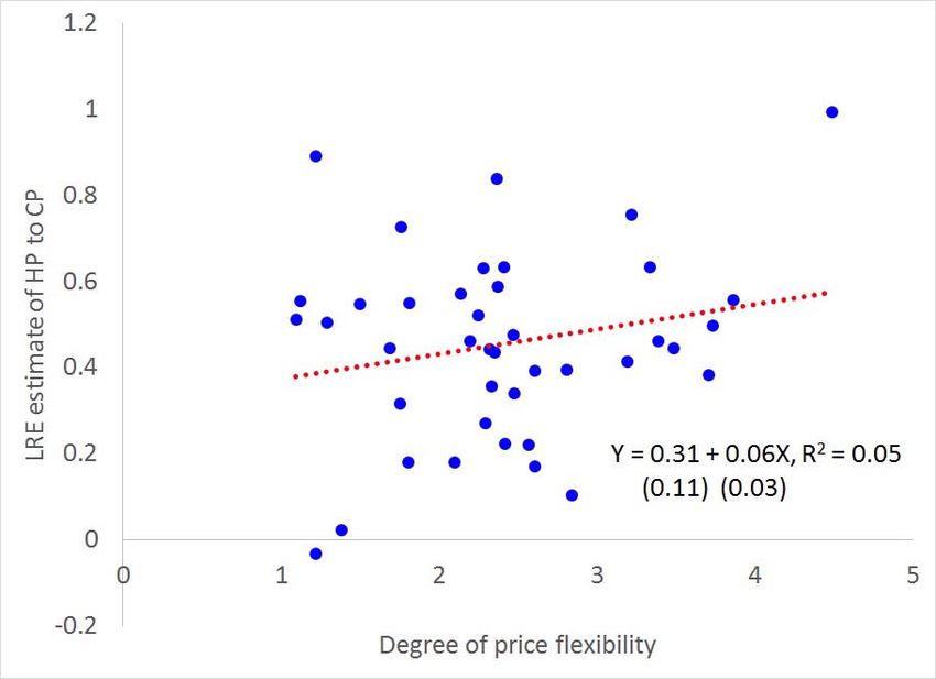
locations in the U.S., they claim that markup variation is a primary explanation for the empirical
patterns; firms raise markups and prices as households become less price sensitive due to a rise in
wealth driven by higher HP.
       Our approach differs from theirs in several aspects, particularly in terms of product diversity
in data, methodology, and impact horizons, which are detailed in Table 1. SV focus on 31 items
including processed food and beverages, cleaning and personal hygiene product. These items are
typically homogeneous nation-wide, and sold in drugstore and mass-merchandise chains that charge
nearly uniform prices across stores, as noted in DellaVigna and Gentzkow (2019). As a result, these
prices may only reflect limited cross-city heterogeneity. Another distinctive feature is that we analyze
the dynamic impacts on CP over time, while SV focus on the cross-sectional elasticity. Finally, while
SV show that the markup effect is a dominant channel, we find that diverse channels are at work
depending on the nature of HP changes. All in all, we believe our paper compliments SV, based on a
further analysis focusing on comparison in Section 4.3.
       Our work is also related to the literature on the consumption effects of HP changes. The significant
relationship between HP and CP found in our paper suggests that HP may have a bigger impact on
the overall cost-of-living than what is simply reflected in its CPI weight. For example, the user cost-
based CPI would not account for the persistent positive effects of HP changes on CP, via wealth
and collateral effects.4 Our results, hence, offer further insights into the role of HP fluctuations in
explaining consumer welfare. Moreover, this paper is relevant to the recent studies identifying changes
in HP as an important driver of increasing geographic price dispersions (e.g., Hsieh and Moretti 2015,
Stroebel and Vavra 2019). For instance, one can infer disproportionate effects of the HP changes on
home owners vs. renters.5
       The remainder of this paper is organized as follows. The next section describes the data set
employed in our study and documents some descriptive analyses of the data. Section 3 provides an
econometric analysis on the impact of housing markets on CP of various products across U.S. cities.
Section 4 discusses the underlying transmission mechanism by utilizing the large variations observed
in CP responses across locations and products. Section 5 concludes the paper. The Appendix contains
a detailed description of our data.
   4
      In constructing its owner-occupied shelter index (comprising 32 percent of CPI), the BLS only measures changes in
the ‘user cost’, or the fair rental value of owner-occupied housing, in a given time period while holding asset ownership
fixed. Owner-occupied housing, however, is also an asset which takes a large portion of the typical household’s portfolio.
As noted by Cecchetti (2007), if the owner-equivalent rent (or implicit rent) is to measure the opportunity cost of owning
rather than renting, then CPI should be based on the price of the house rather than on the rental market.
    5
      Empirical evidence on the effects of HP appreciation on the consumption behavior between homeowners and renters
and its impact on CPs is somewhat mixed. Sheiner (1995) documents a positive effect of HPs on the net worth of young
renters using the U.S. PSID data, while Campbell and Cocco (2007) find that the effect of HP changes on consumption
is lowest and insignificant for young renters, and highest for old homeowners.

                                                            3
2 Data and preliminary analysis
We use the quarterly retail price data published by the Council for Community and Economic Research
(C2ER) for selected U.S. MSAs over the period 1990Q1 to 2015Q4. Originally constructed for the
comparison of living costs across cities for mid-level managers, this survey data set contains retail
prices of individual goods and services quoted inclusive of all sales taxes levied by all jurisdictions. It
is suitable for the purpose of our study for several reasons. First, prices are measured for comparable
items across different locations, and thus, facilitate our cross-city comparison. They are absolute prices
in dollars and cents collected by a single agency for specific goods and services in terms of quality
(brand) and quantity (package), such as gasoline (one gallon, regular unleaded) and beauty salon
(woman’s shampoo, trim, and blow dry). As described in Table A.1 in the Appendix, the products
range from basic food products such as bread and eggs, to manufacturing goods like detergents and
tissues, and to services including medical service and hair-styling.6 Second, the data set covers a long
sample period and wide geographic regions as displayed in Figure 1. While the number of products
included in our data set is smaller than that in the BLS micro-data and grocery store scanner data
(e.g., Nielsen or the IRI Database), it has a longer time series and covers a larger number of cities.
This allows us to construct a long and wide panel that is useful for analyzing the dynamic impacts
on CP. Third, our data set provides actual HP, not in a price index, which enables us to investigate
the long-run relationship between HP and CP within the framework of VECM. This would not be
plausible with popularly-used price indices. Table A.2 lists summary statistics for the 43 products
considered in our study.
We focus on the metropolitan statistical areas (MSAs) because housing markets are often defined
at the MSA level and workers likely consider jobs in the same MSA for commuting, comprising one
labor market (Sinai 2012). The selected 41 cities are well diversified in terms of the relative size,
measured by average per capita income and population, as displayed in Figure 1.7 Together, they
account for significant share of the nation’s wealth, consumption and investment. Summary statistics
for the 41 cities are presented in Table A.3 in the Appendix.
We also draw on many sources for local economic environment and housing market conditions
data that are used for our regression analysis. As listed in Table A.4 in the Appendix, these city-level
control variables include per capita income, unemployment rate, population density, homeownership
rate, financial integration, share of skilled workers, and the measure of housing supply constraints by
6
The products considered here are staples that are regularly purchased, rather than big-ticket items that one might
purchase on an infrequent or once-off basis (e.g., cars, electronics). Refer to Table A.2 for the summary statistics by
products.
7
Due to data insufficiency, major cities like New York, Chicago and San Francisco are not included in our dataset.
4Guren et al. (2020).
It is worth noting the details of two control variables. First, the share of skilled worker is measured
by educational attainment, i.e., the fraction of adults over 25 years old with at least a bachelor’s
degree. A large body of research relates educational attainment to urban and metropolitan prosperity,
such that cities with higher concentrations of bachelor’s degree holders are likely to have higher levels
of income and HP. Second, we use the inverse measure of housing supply elasticity (̂) estimated
by Guren et al. (2020), as a measure of housing supply constraints at the city level. The data are
downloaded from the Adam Guren’s website ( : ). This measure is based
on historical sensitivity of local HP to regional housing cycles.8 See Table A.4 in the Appendix for
the descriptions of other variables.
We illustrate in Figure 2 the relationship between annualized HP and CP both in level (top panel)
and in growth rates (bottom panel) for two selected products (i.e., ‘CORNFLAKE’ on the left and
‘HAIRCUT’ on the right), over the entire sample period.9 As shown in the top panel, there is a strong
positive association between HP and CP in both products. In line with our priors, cities with higher
level of HP (on the horizontal axis) tend to have higher CPs (on the vertical axis). As can be seen
from the bottom panel, however, the positive association is less clear when it comes to the growth
rates of prices; CP growth is not much correlated with HP growth. Nevertheless, as discussed below
this outcome does not necessarily refute a long-run relationship in the growth rates between CP and
HP because there could be a lagged relationship in the growth rates between the two variables. This
justifies our focus on the long-run relationship between HP and CP in our analysis.
3 Empirical analysis
In this section, we quantify the impact of housing market shocks on local CP. To this end, we first
exploit a FAVAR model in which structural aggregate housing market shocks are identified with sign
restrictions as in Jarocinski and Smets (2008) and Abdallah and Lastrapes (2013). The FAVAR model
provides a consistent and coherent framework to look at impulse responses. We then estimate the
dynamic effects of local HP changes on local CP within the framework of VECM.
8
A wide cross-city variation in the HP developments is often attributed to differences in housing supply elasticities (e.g.,
Aastveit et al. 2020, Green et al. 2005). Saiz’s (2010) housing supply elasticity estimates based on land-unavailability
are popularly used in the literature, but they are subject to a couple of serious drawbacks for being a valid instrument.
Alternatively, Guren et al. (2020) develop a measure of city-level housing supply elasticities based on the systematic
historical sensitivity of local HPs to regional housing cycles. It is claimed to address the major problems of the Saiz’s
measure. While the literature generally utilizes time-invariant measures of housing supply elasticities, Aastveit et al.
(2020) show that housing supply elasticities can change over time.
9
The results are qualitatively similar for other products. A complete version of Figure 2 will be available at the online
Appendix.
53.1 FAVAR analysis
3.1.1 FAVAR model
We employ the following FAVAR model in which the joint dynamics of the factors and macroeconomic
variables are modeled as
∙ ¸ ∙ ¸
−1
= 0 + () + (1)
−1
= + + + (2)
where and respectively represent observable and unobservable factors, and is a vector of city-
level price changes of various goods and services. As is common in the literature, the factors ( and
) are assumed to capture common dynamics in . Following the setup in Abdallah and Lastrapes
(2013), we include six macroeconomic indicators as observable factors ( ): (i) real private residential
fixed investment, (ii) aggregate real HPs, (iii) 5-year U.S. Treasury-bond yield, (iv) GDP deflator,
(v) real GDP, and (vi) real personal consumption expenditure. We control for other factors which
may be related to local housing market, i.e., the local labor market condition by including city-level
unemployment rates ( ) in eq.(2).10
We identify aggregate housing demand and supply shocks by imposing sign restrictions, as in
Abdallah and Lastrapes (2013). Our identification strategy assumes that the housing demand shock
will drive both real aggregate HP and the residential fixed investment to the same direction. In
contrast, the housing supply shock moves them to opposite directions. The sign restrictions are imposed
for three quarters after the impact. It is worth noting that the restrictions are imposed neither on
other macro variables in nor on , and we let the data determine their dynamic responses (see
Table 2 for the summary of the restrictions).
Housing market shocks identified in our model reflect a broad range of unexpected changes in the
aggregate housing market. For instance, a housing demand shock can arise due to the implementation
of macroprudential policy measures such as loan-to-value and/or income-to-debt payment ratios. Or,
it could be more broad-based, caused by monetary policy changes. Housing supply shocks constitute
unexpected changes in the costs of producing houses and developing real estate, technological advances,
changes in input prices, and regulatory changes on housing supply. In line with Abdallah and Lastrapes
(2013), we do not further identify the origins of the shocks, but focus on investigating their differential
impacts on local CP.
10
The change in the unemployment rate also captures urban economic performance (e.g., Aastveit et al. 2020). Beraja
et al. (2019) show that price growth was much higher in states with lower unemployment growth relative to those with
higher unemployment growth.
6As in Bernanke et al. (2005) and Boivin et al. (2009), we estimate the FAVAR model based on a
two-step principal component approach: first, estimate the common unobservable factors from by
extracting principal components and rotate the unobservable factors so that they are orthogonal to
; then, augment the common factors to for the estimation of eq.(1). Prior to the estimation, all
variables are standardized to be suitable for a factor model by taking log first-differences to impose
stationarity, except for the 5-year T-bond yield which is first-differenced only. All CPs at the city level
are also in first-differenced logs to represent quarterly growth rates. Once the impulse responses are
estimated for the variables and factors in the main VAR, we feed them back into eq.(2) to investigate
how each shock at the aggregate level propagates to the city-level CP changes. We normalize the im-
pulse responses to represent a demand or a supply shock that increases aggregate housing construction
by one percent at the impact. The impulse responses are estimated for 16 quarters (four years) after
the impact so as to tell whether short-run dynamics resulting from specific shocks sustain for a longer
term period.
3.1.2 The FAVAR results
We first assess whether the aggregate housing market shocks are properly identified. In Figure 3, we
plot the cumulative IRFs of local HP in 41 cities to aggregate housing demand and supply shocks on the
top and bottom panels, respectively. The results corroborate our priors about the effects of aggregate
housing market shocks: positive effects of housing demand shocks and negative effects of housing
supply shocks. Interestingly, the responses differ significantly in persistence; following an aggregate
housing demand shock, local HP rises gradually and persistently to a peak response of more than 1.5%
at the four-year horizon. By contrast, local HP shows a U-shaped response to a supply shock; it drops
for one year to a trough of about 0.3% before starting to revert toward zero subsequently.
Table 3 presents the estimated IRFs, averaged across cities for each product. The left-hand side
reports the average peak cumulative responses over the 16-quarter horizon to an aggregate housing
demand shock, while the right-hand side presents the average trough responses to an aggregate housing
supply shock. The responses to the demand shock is positive in the vast majority of products, with the
average peaks at 0241 percentage points (p.p.). By contrast, the supply shock has negative responses
in most cases, with the average trough impact of −0145 p.p.
Our results illustrate the following points. First, there exists a considerable heterogeneity in the
responses across products. For instance, the price of ‘WINE’ increases at the peak only about 0005
p.p in response to a housing demand shock, while ‘HOUSE PRICE’ rises by 1674 p.p. This large
cross-product heterogeneity is informative about the underlying transmission mechanism of housing
7market shocks to local CP. Second, the wide inter-quartile bands found in many products indicate
the substantial cross-city dispersion of shock impacts. This is likely caused by differences in local
factors (e.g., Moretti 2013, Diamond 2016). To be specific, local distribution costs, such as rents paid
by the retail establishment, wages of the retail workers, transportation and warehousing, must be a
nontrivial component of the retail good and service prices and contribute to the observed cross-city
heterogeneity.11 Finally, we find the stickiness of price responses in most products, as CP respond to
housing demand shocks with some lags, consistent with Abdallah and Lastrapes (2013).
To sum, our results from the FAVAR analysis indicate that city-level CP responds in general
positively to aggregate housing demand shocks and negatively to housing supply shocks, with the
former exerting larger impacts. The size of responses varies considerably across cities and products.
As discussed in Section 4 in more detail, we use such variations to identify the channels through which
housing markets influence local CPs.
3.2 VECM analysis
3.2.1 VECM model
Although intriguing, our FAVAR model analysis focuses on the impact of aggregate housing market
shock, rather than local housing market shock which is of growing interest in the literature. In response,
here we explore how local CPs respond to local HP shocks within the framework of a VECM. The
VECM analysis is suitable for the purpose of our study on several grounds. First, it allows for possible
interactions between HP and CP with less restrictions than the traditional structural model in which
HP is typically assumed to be exogenous.12 This feature of the VECM is appealing to a study like ours
that employs MSA data where the distinction between purely endogenous and exogenous variables is
often difficult to make. Second, the VECM approach takes into account the likely interactions between
CP and HP both in the short run and in the long run. Given that housing market shocks can affect
CPs over time as we have seen from the FAVAR analysis, it is important to measure the long-run effect
of the changes in HPs on the changes in CPs. Third, the VECM approach allows causation to run both
ways between HP and CP and hence it helps us to determine the direction of causality (predictability)
between the two variables. As shown in Figure 2, higher HPs are often associated with higher CPs,
but empirically establishing the causality from HP to CP is challenging because causal relationships
11
Retail prices may also reflect a pass-through of local retail rents or land prices as part of marginal costs (along
with labor costs). However, SV claim that the relationship between retail prices and house prices was driven not by
pass-through of local land prices or rents.
12
Consisting of a system of equations with lagged endogenous variables, the VECM is akin to vector autoregression
(VAR) model except that it includes an error correction term to capture deviation from the long-run relationship between
endogenous variables.
8can run from both sides over time. The VECM analysis permits us to make formal inference about
the leading/causal relationship while controlling for other relevant factors.13
With that said, implicit in our VECM analysis is the assumption that local HP changes are
exogenous without further identifying the shocks that drive the price changes, following much of the
literature. To rephrase, we use HP changes as housing market shocks without identifying its origin,
although they can be driven by either housing supply or demand shocks. Since HP per se may be
the transmission mechanism of housing demand or supply shocks rather than a source of fundamental
shocks, an ideal approach should be to considering how CP and HP jointly respond to appropriately
identified, exogenous shocks.14 Nevertheless, in the dearth of such identified shocks of local housing
markets, the exogenous HP changes can be arguably viewed as an indicator of the changes in local
housing demand, not just because our FAVAR analysis shows the dominance of aggregate housing
demand shock over supply shock, but because housing demand adjusts more quickly in the short run.
We estimate the following bivariate VECM in which HP and CP are simultaneously determined
as well as determining,
∙ ¸ ∙ ¸ ∙ ¸ ∙
X ¸∙ ¸ X ∙ ¸
∆
11 12 ∆−
= + ̂−1 + + ∆− +
∆
21 22 ∆−
=1 =0
(3)
where
and
denote fixed effects and ̂−1 = (−1 − ̂−1 ) is the error correction term cap-
turing the deviation from the long-run equilibrium relationship between HP and CP. The cointegrating
vector (1 −) yields a consistent estimate of the long-run relationship between the two variables. If
there were a deviation from the long-run relationship in the previous period (as captured by the error
correction term, ̂−1 ), then either HP or CP should adjust to correct for the deviation in the current
period. The parameter (or ) captures the speed at which CP (or HP) adjusts to the long-run
equilibrium per period after a shock. If the parameter estimate of (or ) is significant, then CP
(or HP) in the current period moves to correct for the deviation. Unlike the conventional univariate
error correction model, the VECM allows the endogeneity as well as the asymmetry of the convergence
13
Despite these attractive features, the VECM was not much popularly used in the study of housing market mainly
due to the lack of adequate HP data. Because most HPs are in index form, it is challenging for researchers to set up
the long-run cointegration relationship formulated in the error-correction terms. In the CPI data, for instance, both HP
and CP have the same values of 100 in the base year and the corresponding error correction term will be zero for the
cointegrating vector (1,-1). For an exception, see Gallin (2008) who studied the long-run relationship between HPs and
rents using a VECM.
14
In studying the impact of HP changes on retail prices, SV adopted exclusion restrictions by using local housing
supply constraints constructed by Gyourko et al. (2008) and Saiz (2010) as instruments for local HP movements. This
IV approach, however, suffers from a couple of thorny issues. First, the popular measures of MSA-level housing supply
constraints are usually static variables (fixed over time) and hence cannot capture properly the time-varying behavior of
the relationship between HP and CP. Second, housing supply constraints could be a valid but not necessarily exogenous
instrument for HP growth (Davidoff 2013, Guren et al. 2020).
9speed, i.e., 6= , which is useful for determining the direction of causality between HP and CP.
City fixed effects are included in both the cointegrating equation and the VECM to control for many
other factors than wage and labor market conditions that influence CPs at the city level. The lagged
terms of HP and CP contain information on short-run dynamics, such as the cyclicality of HP. We
also augment the current and lagged changes in city-level wage and unemployment rate as control
variables ( = [ ]) in eq.(3). By so doing, we can account for changes in the local economic
fundamentals, cyclicality in the local labor market, as well as labor mobility across cities.15
Since the VECM approach requires establishing a cointegrating relationship between variables,
we first implement a popular unit-root test, the DF-GLS test under the null hypothesis of unit-root
nonstationarity, to the city-level price series to check the prerequisite of a formal cointegration test.
As reported in Table 4, the DF-GLS test fails to reject the unit-root null for all the HP series under
study and in the vast majority of CP series, indicating strong evidence of unit-root nonstationarity
for the price series. In turn, we apply the Hausman-type cointegration test developed by Choi et al.
(2008) to the 1,763 HP-CP combinations in order to examine whether city-level HPs have a long-run
cointegration relationship with CPs. As reported in the last column of Table 4, there is strong evidence
of cointegration between HP and CP as we fail to reject the null hypothesis of cointegration in most
cases at the five percent significance level. The low rejection rate of the null hypothesis of cointegration
indicates a long-run cointegration relationship between HP and CP and hence validates our use of the
VECM approach.
3.2.2 The VECM results
The results of the city-level VECM analysis are presented in Table 5. First of all, we find compelling
evidence that local CPs are influenced by local HPs, but not vice versa. As reported in the left panel
of Table 5 (columns 1-2), ̂ is significant and positive in all products but one, while ̂ is mostly
negative and insignificant. To interpret, the deviation from the long-run equilibrium between HP and
CP is corrected primarily by the adjustment of CP, not by HP. The cross-product average of ̂ is
around 0.194, indicating that on average almost 20 percent of the gap between HP and CP is reduced
each quarter by the adjustment of CP. Not surprisingly, the adjustment speed (̂ ) varies widely across
products, ranging from 0.012 (‘AUTO MAINTENANCE’) to 0.548 (‘LETTUCE’). Interestingly, the
adjustment speed of CPs appears to be faster in perishable products.
15
Local wages and labor market conditions help mitigate the reverse causation from CP to HP. Van Nieuwerburgh and
Weill (2010) claim that the dispersion in MSA-level wages, reflective of local labor productivity, has been large enough
to account for the spatial distribution in HPs. Beraja et al. (2019) also emphasize the importance of local factors such as
local labor market condition in the distribution of prices. Analyzing retail prices across many U.S. metropolitan areas,
however, Coibion et al. (2015) find that changes in retail prices respond little to local unemployment rates.
10The VECM in eq.(3) also permits us to implement the Granger (non-)causality test by looking at
whether or not changes in HP can help predict changes in CP. This is equivalent to testing the null
hypothesis that HP does not Granger cause CP (0 : 6⇒ ) with a standard F-test,
0 : = 21 = 0 for = 1
Likewise, the null hypothesis that does not Granger cause (0 : 6⇒ ) can be formulated
as 0 : = 12 = 0 for = 1 . Beware that rejecting the null hypothesis of noncausality of
HP to CP (0 : 6⇒ ) simply implies that changes in HP is helpful in predicting (forecasting)
change in CPs without providing any further assessment on the strength of the improvement in the
forecast. Columns 3 and 4 in Table 5 report the rejection rates of the nominal ten-percent Granger
causality test for each product. The rejection rate of 0 : 6⇒ is in general quite high in most
products under study, while that of 0 : 6⇒ is relatively low. This result suggests a one-way
Granger causality (or predictability) running from HP to CP, but not the other way around.16
Nevertheless, the inference from the bivariate VECM, which examines each HP-CP pair in each
city separately, could be fragile if the relationship was driven by unobservable common factors. This
concern is legitimate in our case where local prices of a product are likely to be correlated across cities,
possibly through common national factors like national supply chains.17 As a further robustness check,
we apply the panel VECM (PVECM) across all the 41 cities for each product. Following Holly et al.
(2010), we utilize the Common Correlated Effects (CCE) estimator in the PVECM to deal with the
cross-sectional dependence (CSD) and the unobserved common factor issues, after controlling for local
wages and labor market conditions as before. The CCE estimators are based on a multifactor error
structure, which controls for unobserved common factors as well as spatial effects of price changes.18
The right panel of Table 5 reports the PVECM results, which largely corroborate the results
obtained from the city-level bivariate VECM. Albeit not as strong as before, we still find evidence of
the one-way causality running from HP to CP, i.e., CPs are responsive to HP, but not the other way
around.19 The coefficient of ̂ is statistically significant in almost half of the products under study,
16
This outcome is in line with the finding by SV on the causal response of local retail prices to changes in local HPs,
based on different shock identifications.
17
HPs are also likely correlated across MSAs, not just through common macro factors, such as the interest rate, that
affect HPs in all MSAs, but also through spatial effects, i.e., HP changes in a MSA affect those in other MSAs. In
this context, CPs in a MSA can be affected by HP changes in other MSAs. In the presence of the multifactor (both
common factor and spatial effect), the usual OLSE is biased as the error terms are correlated to the common factor of
the explanatory variable by nature.
18
The CCE estimators are constructed using regressions augmented with cross-sectional averages of all dependent and
independent variables. As shown by Pesaran (2006), the cross-sectional averages of dependent and independent variables
effectively control for the unobserved common factors.
19
The weaker evidence of causality running from HP to CP in the PVECM must have arisen from the fact that the
influences of common national factors are effectively removed by using the CCE estimates. This is particularly relevant
for some products that are typically produced nationally (e.g., ‘SHORTENING’).
11while the coefficient of ̂ is significant in no products. Interestingly, the long-run causal relationship
running from HP to CP is found more frequently in food and rent related products that are more
influenced by local factors. Again, a wide variation exists in the speed of adjustment (̂ ) across
products. CPs of some products adjust to HP much faster than those in other products. In general, the
adjustment speed appears to be faster for non-durable products which are typically produced locally
in a more competitive environment, compared to manufacturing goods that are produced nationally.
The fastest adjustment speed was found in ‘GROUND BEEF’ (almost 39 percent per quarter), while
the adjustment speed is very slow for ‘MEN’S SHIRT’ (less than 1 percent per quarter). As presented
in the last column of Table 5, the long-run effect (LRE) of a unit-shock of HP onto CP also varies
widely from 0.024 (MAN’S SHIRT) to 0.994 (GASOLINE), i.e., the local gasoline price is a lot more
responsive cumulatively to a change in local HP. The average LRE across products is around 0.46, i.e.,
a 10% increase in HPs is associated with around 4.6% increase in CPs. This estimate is higher than the
cross-sectional elasticity of CP to HP (0.15-0.20) reported by SV. As discussed in more detail in Section
4.3, the difference between the two studies stems from a variety of sources, including the differences
in data coverage, identification of shocks, time horizons of shock impacts, and methodologies.
4 Transmission channels of housing markets to CPs
Our analysis so far suggests that the impact of housing market shocks on local CP is nontrivial and
persists over time. More importantly, substantial heterogeneity was found in the response across cities
and across products. This heterogeneity contains useful information about underlying transmission
mechanism. Previous literature has featured a range of transmission channels, some of which can be
simultaneously at work to different degrees, resulting in the observed heterogeneous responses. In this
section, we attempt to disentangle those different channels based on the cross-city and cross-product
heterogeneities found in our data. To that end, we conduct a second-stage regression analysis to gauge
the importance of competing transmission mechanisms by relating the estimated impacts to a variety
of city- and product-specific characteristics.
4.1 Transmission mechanisms of housing market shocks to CPs
The channels through which HP changes affect consumption has garnered enormous and growing
attention from both policymakers and academic researchers. The existing literature offers two major
channels through which changes in HP affect consumption spending: the (i) wealth effect and (ii)
collateral effect. According to the wealth effect, higher HP increases consumption spending by raising
12homeowners’ wealth.20 In the collateral effect, higher home values affect consumption by allowing
credit-constrained households to borrow more against their homes (e.g., Campbell and Cocco 2007,
Iacoviello 2005). Its strength therefore hinges on the friction of local financial market condition (e.g.,
Abdullah and Lastrapes 2013).21 Since these demand-pull channels imply higher demand for products
upon HP appreciation, they further point to positive effects on CP.
On the supply side, the recent work by SV highlights the mechanism that works via pricing practices
of firms and/or local retailers; an increase in HP leads to higher CP as firms raise their markups while
taking advantage of homeowners’ lower price sensitivity ((iii) markup effect). Another supply-side
channel works through the production costs that are directly affected by local housing market ((iv)
local cost effect). The strength of local cost effect likely depends on the degree of overall housing
supply constraints in the area (e.g., Gyourko et al. 2008). Since both markup and local cost effects
are related to the firms’ costs, we call them a cost-push channel.
We now explore how these diverse channels are at work in our data. We regress the estimated
cumulative IRFs of CP from the FAVAR model in Section 3.1 onto a set of observable city and product
characteristics. The city characteristics considered here include per capita income, population density,
fraction of skilled workers, homeownership rate, unemployment rate, remoteness, financial integration,
and housing supply constraint (see Table A.4 in the Appendix for the details regarding their definitions
and sources). For the product characteristics, we consider flexibility of price adjustment and production
proximity, which have been identified as plausible factors in the literature (e.g., Parsley and Wei 1996,
O’Connell and Wei 2002).
Table 6 summarizes how each transmission mechanism under consideration is reflected in city
and product characteristics. First, we expect a stronger wealth effect in the cities with a lower per-
capita income or a smaller share of skilled workers. Households in such cities more likely exploit HP
appreciation to finance consumption expenditures and hence increase CP. The wealth effect would
also be stronger in the cities with a higher homeownership rate, as homeowners may respond more
than renters to the HP changes. Second, the collateral effect is expected to be weaker in the cities
with a larger share of skilled workers who are less financially constrained (e.g., Berger et al. 2018,
Lustig and Van Nieuwerburg 2010). It is also likely stronger in the cities with a tighter linkage to the
national banking system, with which homeowners can have easy access to home equity.22 Third, the
20
Abdallah and Lastrapes (2013), however, argue that this ‘pure’ wealth effect of HP on aggregate spending might not
be strong because the asset value of home is in general offset by the implicit (or explicit) rental cost of using the home.
21
Since housing can be used as loan collateral, it allows borrowing constrained homeowners to smooth consumption over
the life cycle, provided that households are not borrowing constrained (Campbell and Cocco 2007). Credit constraints
may be particularly binding for some individuals like young households who are looking to transition from rental markets
to the owner-occupied market.
22
In a similar context, Abdallah and Lastrapes (2013) maintain that consumption spending is more sensitive to housing
13markup effect is expected to be inversely related to city population density, where firms would have
lower pricing power as markets are more competitive (e.g., Handbury and Weinstein 2015). Instead, it
is likely stronger in the cities that are geographically and economically isolated, which makes it easier
for firms to exercise their pricing power. It would be also negatively related to local unemployment,
as markup rates are well-known to be cyclical (see for example, Nekarda and Ramey 2013). Finally,
we expect stronger local cost effects in the cities where housing supply constraints are more stringent,
thus HP changes results in larger impacts on local costs such as rents.
Of the two product characteristics we consider, the first one is the price adjustment flexibility.
It can be viewed as a proxy for the degree of market competition, as prices are likely adjusted more
flexibly in more competitive markets. Since markup rates are expected to be lower in more competitive
markets, the price flexibility is also related (negatively) to the markup effect. In our analysis, we divide
the products into three groups based on the degree of price flexibility: (i) most flexibly priced; (ii)
medium flexibly priced; and (iii) least flexibly priced groups.23
The second product characteristics is the production proximity to marketplace, which reflects
product-level market frictions as well as markup rates. For example, as many of the nationally pro-
duced and distributed products are branded, firms producing those products can exercise more pricing
power. In the case of locally-produced products, the price setting power of producers would be limited
because consumers would have lower allegiance to specific products. Hence, we expect the markup
effects would be negatively related to the production proximity. In contrast, the local cost channel is
expected to be stronger for locally-produced products. Since the latter, such as milk, are difficult to
transport, they are more influenced by local production costs like rent. Following O’Connell and Wei
(2002), products are also sorted into three groups based on the production proximity: (i) generally
not locally-produced products (Category A); (ii) maybe locally-produced products (Category B); and
(iii) always locally-produced products (Category C).
4.2 Regression analysis for identifying transmission mechanisms
We conduct the following cross-section regression analysis in which the cumulative IRF estimates from
the FAVAR models are regressed on the set of the aforementioned city and product characteristics
variables,
2
X
0
= + + +
for = 1 43 = 1 41 = 0 4 (4)
=1
demand shocks in states with better-developed financial institutions.
23
We obtain the price flexibility data for our products by utilizing the extensive data set constructed by Nakamura
and Steinsson (2008). See Table A.1 for details.
14 represents the h-year median cumulative effect of housing market shocks on the price of
where
the product in city . denotes a product dummy variable for three product groups based on
either the price flexibility (for the housing demand shock) or the production proximity (for the housing
supply shock). is the set of city characteristics discussed earlier.
is the error term that can
be cross-sectionally correlated and possibly heteroskedastic. Because standard heteroskedastic robust
standard errors may overstate the true standard errors in the presence of a high degree of clustering
among the city and product combinations, we use robust clustered standard errors.24 We conduct two
sets of regression analyses with the IRFs to housing demand and supply shocks separately.
The regression results are reported in Table 7. We first note a difference in the significance of
explanatory variables between the two different housing market shocks. For housing demand shocks,
city characteristics such as the share of skilled workers and remoteness turn out to be consistently
significant in explaining its pass-through. The result of the skilled worker share is consistent with
the finding by Moretti (2013) on a systematic positive relationship between HP and the number of
college graduates in a city. These, however, do not much line up with the demand-pull channel. The
insignificance of per capita income and the unexpected negative sign of the share of homeownership
run counter to the wealth effect argument, while the insignificance of financial integration further
weakens the relevance of the collateral effect.25 Nonetheless, we find that housing demand shocks
have significant impacts on CPs in the products whose prices are adjusted more frequently, in line
with our prior that firms would respond quickly to the increased product demand from the wealth or
collateral effects.26 Collectively, our results partly support the demand-pull channel as it is at work
in the transmission of housing demand shock across products, but not necessarily across space.
Turning to the results for supply shocks, we no longer see the significance of the skilled worker
share. Instead, housing supply constraint and homeownership rate are consistently significant for
explaining the cross-city differences in their pass-through. Hence, they provide evidence supporting
the local cost and markup effects, respectively.27 For the product characteristics, the result implies
that the supply shocks spill over significantly more to the locally-produced products, compared to the
nationally-produced ones. This outcome further supports the local cost effect, but not the markup
effect. Taken together, the transmission mechanism of housing supply shock is better aligned with the
24
Since the impacts of housing market shocks are more likely correlated across cities for a given product, rather than
across products for a given location, standard errors are clustered by observations by cities rather than by products.
25
This result differs from Abdallah and Lastrapes (2013) who find supportive evidence of the collateral effect using the
state-level consumption expenditure data.
26
This outcome, however, is at odds with the recent finding by Beraja et al. (2019) that nominal wage rigidity plays a
more important role than price stickiness in the transmission of local economic shocks during the Great Recession. The
authors also argue that prices respond very quickly to changes in local economic conditions, but not to housing market
shocks, which is quite different from what is found in the current study.
27
The homeownership rate is generally higher in smaller cities where firms’ market power is stronger.
15cost-push channel via local cost effect. The markup effect is at work at the city level, but not at the
product level.
In sum, our results suggest that the nature of housing market shocks matters for the transmission
mechanisms. Whereas housing demand shock is mainly transmitted to CP through the demand-pull
channel, housing supply shock is transmitted primarily through the cost-push channel. Moreover, it
seems improbable that any one transmission mechanism in isolation would be sufficient to explain the
impact of housing markets on local CPs.
4.3 Further discussions on the empirical findings
As noted in the introduction, our paper is closely related to the recent work by SV. Despite the similar
conclusions reached about the impact of HP and CP, the two studies differ, in particular with respect
to the details of the relevant transmission mechanism. To begin, while SV highlight the changes in
markups as the primary channel, we find that the markup effect is at work only in the transmission
of housing supply shocks. Moreover, SV did not find the relevance of local retail rents or land prices.
Furthermore, whereas SV find that HP changes affect the retail price mainly through homeowners, we
show that homeownership mitigates the transmission of a housing demand shock, but intensifies the
effects of a housing supply shock.
In addition, the results from two studies also differ with regard to the role of price flexibility. We
find that housing demand shocks transmit faster to the products whose prices adjust more frequently.
By contrast, SV contend that firms’ pricing-to-market practice is the primary channel, as firms charge
higher prices in locations with higher HP. Since markup rates would be smaller for the products with
frequently-adjusted prices, one might infer that our findings do not accord with theirs regarding the
role of price flexibility.
To ensure that our results on the role of price flexibility are not an artifact of specific empirical
methods, we further delve into this issue using the results obtained from the VECM analysis. Specifi-
cally, we examine the relationship between the degree of price flexibility and the estimated adjustment
speed of CP (̂ in eq.(3)) across products. Intuitively, how fast prices can adjust to a shock might
hinge on how quickly CP can correct for the deviation from the long-run equilibrium. More impor-
tantly, one would expect a faster adjustment of CP to the deviation in the products with more frequent
price adjustment. As illustrated in the top panel of Figure 4, we indeed find a positive association
between the adjustment speed (̂ ) and the degree of price flexibility across 41 products. We also
look at the relationship between the price flexibility and the long-run effect estimates from the Panel
VECM, reported in the last column of Table 5. As shown in the bottom panel of Figure 4, we again
16find a positive association. These results reinforce our previous findings from the FAVAR model that
price flexibility plays an important role in the transmission mechanism.
That being said, the difference between the two studies could arise from a variety of sources,
including data coverage, econometric methodology, and time horizon of shock response, as summarized
in more detail in Table 1. For instance, while we employ the data set covering a wide range of products
including food, manufacturing goods, and services, SV focus on tradable goods only that are generally
sold in grocery stores or drugstores. Those goods are typically produced nationally, and hence, are
not much susceptible to local shocks. This may explain why the significant effect of local cost is found
in our study, but in SV. We also note that the two studies focus on different time horizons. While
SV focus on the cross-sectional elasticity, our main interest is in the cumulative long-run effects. The
latter can be quite different from the former, as shocks can take time to propagate and their impacts
may exhibit some nonlinear patterns over time.
Differences in the sample periods also turn out to be consequential. To investigate this issue, we
estimate the elasticity of local retail prices to HP movements in the spirit of SV (eqs.(1)-(2) in p.1409)
using our data. For this exercise, we focus on the 11 processed food-related products in our data,
to retain similarity with the ones considered by SV. Also, we use the housing supply elasticity from
Guren et al. (2020) as an instrument, instead of the Saiz’s (2010) measure employed by SV. We find
that the average elasticity of local retail prices to HP is around 10.7 percent over the period 2001-2011,
which is much smaller than the cumulative long-run effect found in Section 3.2, but close to the range
of 15-20 percent reported by SV.
We further look at the stability of our findings over time using a rolling window estimation. Figure
5 plots the mean and interquartile ranges of the long-run effects among 43 products, estimated from
the Panel VECM using a 10-year rolling window. As displayed in figure 5, the mean has been stable
around 0.4 until the period of 1998-2007 when it started rising to around 0.6 and then declined steadily
toward zero.28 A similar pattern is noted in the interquartile ranges of the estimates, suggesting that
the time-varying behavior is significant across all products under study. Interestingly, the time-varying
estimates appear to align with the housing boom-bust cycle in the 2000s (e.g., Gelain et al. 2018).
Specifically, the pass-through was stronger during housing boom when HP rose fast, then weakened
during housing bust period. This finding lends credence to the claim by Guren et al. (2020) that it
is challenging to discern between a cyclical pattern and the causal relationship between HP and CP
based on a single cross-section regression. All in all, we view that our paper compliments and extends
28
The decline in the responsiveness of CPs to HP in recent years might have come from the increased pricing power of
firms in the U.S. due to reduced competition in many industries. In a more concentrated market, firms can time their
pricing to maximize profits and thus absorb housing market shocks. Relatedly, Heise et al. (2020) attribute the decline
in the pass-through of wages to goods prices to rising import competition and increased market concentration.
17the work by SV.
5 Concluding remarks
Housing markets have long been recognized to be important for the overall economy, in particular
due to the potential influences of housing values on consumption spending. Yet, few studies have
focused on the impact of housing markets on local CP. Given that housing typically takes up a major
proportion of household net worth for most homeowners, a change in HP could have a significant effect
on CP possibly through consumption spending and shopping behavior (e.g., Aguiar and Hurst 2007,
Kaplan and Menzio 2013). HP may also affect CP via the cost of local services or rents especially in
cities where housing/land is more expensive.
In this paper, we investigated whether, to what extent, and through which channels housing
markets affect local CP, using retail price data collected for the selected U.S. cities over the past 25
years. Within the framework of FAVAR and VECM, our empirical analysis revealed that most local
CP were highly responsive to the changes in local HP, but not the other way around. Controlling
for city-level income and local labor market conditions, we found that on average a 10% rise in HP
leads to around 4.6% increases in CP over time. The leading/causal effects of housing markets on
local CP, however, differ markedly depending on the nature of shocks. While housing demand shocks
have persistently positive effects on CP, supply shocks exhibit transitory negative impacts. Significant
heterogeneity was also found in the size of effects across products as well as locations. We exploited
the heterogeneous responses to explore the potential underlying channels of pass-through by linking
the estimated responses of CP to a set of observable factors identified in the literature as reflecting
underlying transmission mechanisms. We found much stronger responses of CP to the housing demand
shocks in the cities that have higher shares of skilled workers and in the products whose prices are
adjusted more frequently. The responses to the housing supply shocks turned out to be stronger in
the cities with tighter housing supply regulations and for the locally-produced products. Collectively,
our results support the demand-pull channel for the pass-through of the hosing demand shock, and
the cost-push channel for the hosing supply shock.
Our findings had further implications on the measure of cost-of-living and consumer welfare. Hous-
ing market fluctuations have an impact on CPI directly by affecting the shelter index (or user cost)
and indirectly through the spillover effects on local CP over time. Together, HP may have substantial
influences upon the overall cost-of-living and consumer welfare. Understanding the link between HP
and CP also offers useful insights into the geographic dispersions of cost-of-living and thus geographic
economic inequality (e.g., Hsieh and Moretti 2015). Our result that homeownership mitigates the
18You can also read