Integrated Train Rescheduling and Rerouting during Multidisturbances under a Quasi-Moving Block System - Hindawi.com

Hindawi
Journal of Advanced Transportation
Volume 2021, Article ID 6652531, 15 pages
https://doi.org/10.1155/2021/6652531

Research Article
Integrated Train Rescheduling and Rerouting during
Multidisturbances under a Quasi-Moving Block System

 Peijuan Xu ,1 Dawei Zhang ,2,3 Jingwei Guo ,4 Dan Liu ,1 and Hui Peng 1

 1
 School of Transportation Engineering, Chang’an University, Xi’an 710064, China
 2
 School of Automobile, Chang’an University, Xi’an 710064, China
 3
 State Key Laboratory of Traction Power, Southwest Jiaotong University, Chengdu 610031, China
 4
 School of Energy Science and Engineering, Henan Ploytechnic University, Jiaozuo 454003, China

 Correspondence should be addressed to Dawei Zhang; dwzhang@chd.edu.cn

 Received 18 November 2020; Revised 24 February 2021; Accepted 18 March 2021; Published 8 April 2021

 Academic Editor: Keping Li

 Copyright © 2021 Peijuan Xu et al. This is an open access article distributed under the Creative Commons Attribution License,
 which permits unrestricted use, distribution, and reproduction in any medium, provided the original work is properly cited.

 It is known that it is critical for train rescheduling problem to address some uncertain disturbances to keep the normal condition
 of railway traffic. This paper is keen on a mathematical model to reschedule high-speed trains controlled by the quasi-moving
 blocking signalling system impacted by multidisturbances (i.e., primary delay, speed limitation, and siding line blockage). To be
 specific, a mixed-integer linear programming is formulated based on an improved alternative graph theory, by the means of
 rerouting, reordering, retiming, and train control. In order to adjust the train speed and find the best routes for trains, the set of
 alternative arcs and alternative arrival/departure paths are considered in the constraints, respectively. Due to this complex
 NP-hard problem, a two-step algorithm with three scheduling rules based on a commercial optimizer is applied to solve the
 problem efficiently in a real-word case, and the efficiency, validity, and feasibility of this method are demonstrated by a series of
 experimental tests. Finally, the graphical timetables rescheduled are analysed in terms of free conflicts of the solution. Con-
 sequently, the proposed mathematical model enriches the existing theory about train rescheduling, and it can also assist train
 dispatchers to figure out disturbances efficiently.

1. Introduction disruptions for the railway system. Furthermore, certain
 articles focused on the self-learning decision technology [2]
High-speed railway faced a rapid development in the world or decision support system [3] to enhance the robustness of
and showed competitive advantages in the passenger market, timetables by the means of iteratively evaluation from
due to its better performance in safety, fast speed, and ef- subsequent time horizons or the so-called offline railway
fectiveness. However, some inevitable disruptions deviate traffic dispatching.
actual train running lines from its original planned lines in Those strategies usually aim at minimizing operation
time/space horizons. As delay time degenerates satisfaction conflicts and train delays for a single/double-tracked railway
of passengers to some degree, it is essential to explore and line/network area on operational conditions and accident
carry out some optimal solutions/measures to recovery characteristics [4]. However, train rescheduling and
normal conditions of railway traffic. rerouting are often applied to a multistep formulation or
 In recent years, train rescheduling problem is one of hot multi-iterations, due to the complexity of this problem [5].
research topics in railway operation and management. In order to solve the negative influence of disruptions/
According to the state-of-art research outcomes, retiming, disturbances effectively, mathematical formulation is proved
rerouting, reordering, and cancelling trains are mainly four to be one of common methods by describing railway op-
kinds of measures [1], which are used to mitigate the eration as a series of constraints, e.g., integer programming
negative influences resulted from disturbances or (IP) [6] model, mixed-integer programming (MIP) model

2 Journal of Advanced Transportation

[7], and alternative graph (AG) model [8]. From the aspect Concerning above analysis, a mixed-integer linear
of different granularities of railway infrastructure or trains programming (MILP) model based on an improved alter-
activities, current existed optimal mathematical program- native graph related to Chinese high-speed railway traffic is
ming can be divided into two groups, i.e., macroscopic established to enrich real-time train rescheduling methods
model and microscopic model. It is common that the mi- by involving rerouting, retiming, and reordering simulta-
croscopic models are applied on a (part of ) independent neously in this paper. The model complements the opti-
railway line impacted by disturbances or minor disruptions. mization model proposed by Xu et al. [18] which focuses on
On the other hands, the macroscopic is able to solve a wider train rescheduling under speed restriction and neglects train
railway area, e.g., a regional network, multitracked area, and rerouting. This paper makes the following contributions:
a comprehensive central junction impacted by disruptions
 (i) A mixed-integer linear programming (MILP)
[9]. The macroscopic model treats railway stations and
 model is established to solve the real-time
segments (i.e., the track between two consecutive railway
 rescheduling problem for the Chinese high-speed
stations) as basic independent units. However, the micro-
 railway traffic, under the combined influence of
scopic model takes signals along the rail track, switches, and
 primary delay, the disruptions related to speed
block sections fully into consideration [10]. The macroscopic
 limitation, and the blockage of siding lines. The
model is good at addressing some serious disruptions
 combination of disturbances is common in real-
[11, 12], but it may ignore some conflicts among trains or
 world railway operation activates and is studied
infrastructure, whose solution cannot be used for practical
 seldom for its complexity, as most as we know.
dispatching work directly.
 Concerning this defect and characteristics of the quasi- (ii) We improved the general job-shop model to achieve
moving block signalling system, herewith, we mainly focus train retiming, rerouting, and reordering, and speed
on applications related to microscopic models. management simultaneously, where the constraints
 Alternative graph, a kind of microscopic model, is widely related to alternative paths in railway stations are
used to deal with the influence caused by mirror/slight erected according to the “Big-M″ principle. Fur-
disruptions/disturbances in a railway system. In the model, thermore, the train entrance path and departure
occupation relations between trains and block sections are path in railway stations area are computed from the
seen as a job-shop scheduling problem, which can be figured view of rail track circuit.
out by alternative graph [13]. When alternative graph theory (iii) Due to the difficulty of model, a two-step procedure
adopts rerouting in railway traffic management, some with three kinds of scheduling rules are applied,
heuristic algorithms, i.e., tube search [14] or neighborhood such as space headway, headway time interval, and
search [15], are usually designed to overcome the HP hard free-conflict rule. In the real-world high-speed
problems. Furthermore, a variety of objective functions have railway experiments, it is proved that this solving
been studied and analysed, which include the minimization method can figure out the solution with good
of secondary (consecutive) delay and final delay (tardiness), quality in an acceptable computation time.
combined with sophisticated multiobjective optimization
 The detail content of this paper is organized as follows.
framework in [16]. Meanwhile, a practicality and validity of
 Section 2 explains the disruptions studied and the basic
alternative graph for reducing the delays are tested. Besides,
 methodology, and the proposed mathematical model im-
most of those applications of alternative graph focus on the
 proved is built to minimize delay times and times of
fixed-blocking system. As most as we know, few papers
 changing routes in Section 3. Furthermore, the experimental
studied the moving blocking system [17] and quasi-moving
 test, solving method, and the result analysis are given in
block system [18]. Xu et al. [18] applied a set of alternative
 Section 4. Finally, conclusions and directions for future
arcs to illustrate the characteristics of the quasi-moving
 research are reported in Section 5.
block system in the Chinese high-speed railway system, but
the rerouting was not involved in the model. Furthermore,
the smooth of train speed curves is optimized by train 2. Problem Description and Alternative
control and traffic management at one iteration [19]. From Graph Theory
the aspect of high-speed train rescheduling problem, the
 2.1. Problem Description. Some inevitable perturbations,
detailed train speed trajectories are considered [20], where
 which are caused by some infrastructure failures, bad
only 2 trains operating on a part of railway line with two
 weather condition, or human errors, cause conflicts between
stations effected by speed restriction are studied in the
 trains or infrastructure. The abnormal condition is unable to
experimental test. On the other hand, an MIP model based
 meet the requirement of trains in full-speed, thus lower
on a stochastic optimization method is established to handle
 running speed in the area impacted is executed, or rerouting/
disturbance on a high-speed railway [21]. Nevertheless, the
 detour is applied to avoid the broken track area. In this
microscopic model is subject to some defects in dealing with
 paper, disturbances studied refer to the combination of
some serious disruptions in the railway system. In order to
 primary delay, blockage of siding line (s), and speed limi-
improve the generalization and robustness of real-time
 tation (s) in segment (s), illustrated in Figure 1:
Chinese high-speed train rescheduling methods, it is es-
sential to consider rerouting, once some track section is (1) Primary delay: before trains enter the given railway
blockage. line, some delay times of trains were generated in

Journal of Advanced Transportation 3

 Time
 13:00 14:00 15:00
 Station A
 Space

 Speed limitation Siding
 line
 Main line 1
 Station B 2
 Unavailability of a siding line 3

 Speed limitation

 1
 Station C Main line 2
 3
 Unavailability of a siding line Siding
 line
 Primary delay
 Station D
 1 2 3 4 5 6 7 8 9 10 1112 13 14 15 16 17 18

 Figure 1: Illustration for multidisturbances.

 their previous routes. In Figure 1, the actual running deteriorate the solving process of the problem and increase
 line of train no.2 (train numbers are listed at the the probability of occurrence of conflicts between trains.
 bottom of Figure 1) switches from the red dash line
 to the red solid line, due to the input of primary
 delay. 2.2. Alternative Graph Theory and Job-Shop Scheduling
 (2) Disturbances related to speed limitation: in Problem. In general, train operation can be seen as a job-
 high-speed railway system, once bad weather con- shop scheduling problem, and the occupation relationship
 dition (i.e., heavy rain/snow, strong wind, and fog), between the train and the block section is similar with the in-
 switch/signalling failures, and any other infrastruc- process of a good in a machine. In this way, high-speed rail
 ture failures occur, one of common efficient response line can be divided into many sections according to the
 actions is to force high-speed trains to reduce their signals or track circuits, and each section can only be utilized
 speeds in the impacted area. Therefore, extra running at most one train at the same time. When two more trains
 time is generated by the speed limitation. The speed apply for one section simultaneously, there is a sequence
 limitations studied can vary from different time decision process to decide which train has the priority to use
 spans, geographical spans, and different speed levels the section. The latter train can only use the section after it is
 in this paper. There are two speed limitation cases released by the former train. As shown in the top of Figure 2,
 shown by the shaded rectangles in Figure 1, where there are three trains of the same direction going to pass a
 trains nos. 5, 6, 7, 8, 10, 13, 14, 15, 16, 17, and 18 are railway station and the scheduled paths of trains t1 , t2 , and t3
 impacted. are 1-2-3-6-7-8-9, 1-2-3-5-7-8-9, and 1-2-4-8-9, respec-
 tively. Thus, train t1 and train t2 are designed to stop and
 (3) Blockage of siding line in railway station: sometimes
 dwell at siding in Sections 6 and 5, respectively. Train t3 is a
 siding line in a railway station is blocked by infra-
 passing-through train by main line (Section 4). Further-
 structure failures, maintenance activities, or pas-
 more, the relationship between trains and railway infra-
 senger activities, so all trains cannot dwell on the
 structure is represented in the bottom of Figure 2, which
 impacted line for passenger alighting or boarding
 manages to transfer the railway operation activities into an
 activities. Thus, the original plan for the usage of the
 alternative graph to optimize occupation sequence of trains.
 impacted siding line should be adjusted to avoid
 To be specific, the node presents railway block section, and
 potential conflicts or accidents, as well as their en-
 the outgoing arc defines the movement of one train between
 trance path and departure path. As shown in Fig-
 two neighboring block sections, and the operation time of
 ure 1, when the siding lines blocked in station B
 each movement (/arc) refers to the running time/entrance
 (siding line 2) and station C (siding line 3), re-
 time/departure time/headway time of the outgoing section,
 spectively, and trains nos. 5, 6, and 7 or train nos. 14,
 which is the weight of each arc. In terms of arcs, the solid arc
 15, and 18, which are planned to dwell in blockage of
 is called fixed arc, which can determine train routes
 siding lines, have to change their siding lines in
 according original plan, and the red dash arcs are the en-
 advance. Undoubtedly, making new arrival path and
 trance deifications for trains, whose weights refer entrance
 departure path are essential to adjust the siding line.
 times of trains scheduled by the timetable while the planned
 As mentioned above, the disturbances studied in this departure times are depicted by green dash arcs which re-
paper are a complicated combination of primary delay, quire that trains cannot leave the station until the departure
speed limitation, and blockage of siding line. They time. Last but not least, the pair of dark dash lines with a red

4 Journal of Advanced Transportation

 t1
 6
 t2
 7
 3
 5
 t3 8
 2
 9
 1 4

 (a)
 6
 1 2 3 7 8 9 10
 t1

 0 5
 1 2 3 7 8 9 10
 t2

 t3 1 2 4 8 9 10

 (b)

 Figure 2: Alternative graph with two trains in one railway station.

circle at their crossing defines a pair of alternative arcs, Direction
which is used to determine the train order for the usage
priority to the same rail section. In detail, for the potential 10 11 12 13 14 15
conflicts caused by the same section occupation between t1
different trains (such as Section 2 and Section 3 for those
three trains in Figure 2), there are three pairs of alternative
arcs which are designed to avoid potential collision between 10 11 12 13 14 15
 t2
different trains. Considering the requirements of switches,
sections, or signals, the headway time between two con- Figure 3: The alternative arcs for headway interval.
secutive trains is treated as the weight of each pair of al-
ternative arcs. Consequently, the headway time of alternative
arcs ((2, 3), (2, 4)) and ((8, 9), (8, 9)) values to required objective: min : ωn − ω0 , (1)
headway time. In terms of the best solution, the minimum of
maximum time from entry node to exit node is the critical ωi,q − ωi,p ≥ fpq , ((p, q) ∈ F), (2)
route (the blue dash line) to get the better solution with more
capacity conservation.
 In respect of the requirement of the quasi-moving block ωj,q − ωi,p ≥ δpq ∨ ωi,k − ωj,h ≥ δhk ((p, q), (h, k) ∈ A),
system, a new space interval restrict is as well taken into (3)
account to keep safety distance for two continue trains in
open track area. In particular, when a train wants to enter a ωj,q − ωi,p ≥ 0∨ωi,q − ωj,p ≥ 0, p ≥ q + ξ, βξ,LaterTrain,q � 1 .
given section with a certain speed, there must be enough
empty sections corresponding to speed level in front of this (4)
train to keep safety in case of emergency braking. A series Constraints (4) can be transferred into the following two
pairs of alternative arcs of each train were generated to constraints:
demonstrate different speed levels for the train on a section
[18]. For instance in Figure 3, the red, purple, origin, blue, ωj,q − ωi,p ≥ − 2 − μi,j − βξ,j,q M, (5)
and green dash lines represent speed level 1, 2, 3, 4, and 5,
respectively, and the bigger the speed level is, the more the ωi,q − ωj,p ≥ − 1 + μi,j − βξ,i,q M, (6)
free section in front required. Obviously, this kind of al-
ternative arcs exists in the segment between two consecutive where ∀i, j ∈ T, ξ ∈ B p, q ∈∈S: i≠j, q � p + ξ.
trains. The ambition of this model is to reduce traffic tardiness,
 Based on the alternative graph theory, all of constraints shown by equation (1), where ωn and ω0 denote the arrival
related to train operations are transformed into a network time of the last train at the end node and the start time of the
graph, and all the arcs in the network graph can be rep- first train at the original, respectively. In the final solution,
resented as mathematical constraints. The detailed formu- each train finds a path, which consists of nodes and arcs, and
lation is shown as follows: the minimum of the longest path is the critical path, which

Journal of Advanced Transportation 5

determines the quality of rescheduled timetable directly. (1) The given disturbances cannot result in cancelation
Constraints (2) relate to fixed arcs, which is used to control of train (s) in any time.
the running time/arrival time/departure time for each train (2) Parameters of speed limitations and blockages of
on each section (the fixed arc), where, fp, q denotes the siding lines are known once they happen.
minimal running time to pass through one section, and ωi,q
 (3) Passing-through trains are forbidden to change their
is the start time when train i utilizes block section q. F is the
 routes in stations. Only those trains which are
set of fixed arcs, and (p, q) represents a fixed arc. In this
 scheduled to stop can change their routes in the
way, the requirements of trains’ entrances of the original,
 planned stop stations.
primary delays, and departure times can be formulated by
those constraints. On the other hand, alternative arcs are The parameters of trains operation, railways lines, and
described by constraints (3), where δpq and δhk represent technical activities are described as follows: t, i, j (t, i, j ∈ T)
minimal headway time interval to keep trains use the denote indexes of trains, and T is the set of trains. s, p, q (s, p,
sections of potential conflicts separately. It should be noted q ∈ S) denote indexes of block sections, and S is the set of
that A is the set of alternative arcs and ((p, q) and (h, k)) is a block sections. A and F denote sets of alternative arcs and
pair of alternative arcs. Furthermore, there is a disjunctive fixed arcs, respectively. ξ denotes the speed levels of the train,
relationship in constraints (3); in other words, only one i.e., 1, 2, 3, 4, and 5, and the bigger the value is, the faster the
subconstraint is tight constraint during solving process. train runs. y is the index of speed limitation case, and M is a
Considering the features of train speed and their safety big enough integer. The decision variables in the model are
braking distance, constraints (4) are used to deal with those shown as follows:
alternative arcs (i.e., arc (10, 11), (10, 12), (10, 13), (10, 14), ωt, s: the start time when train t utilizes block section s.
and (10, 15) in Figure 3), with speed levels in the open track zt, s: binary decision variable, i.e., if zt, s � 1, train t uses
area. To be specific, the distance headway to be kept free section s; otherwise, section s is not used. Section s is among
between two consecutive trains depends dynamically on sections in railway station area, i.e., (t, s) ∈Rt, station, where Rt,
the speed level of the following train. We thus require that station is the set of block sections in station area which can be
at least ξ block sections should be kept free between two used by train t.
consecutive trains, when the second train runs at the speed λi, j, p, q: binary variable which describes the sequence
level ξ (βξ,LaterTrain,q �1). βξ,LaterTrain,q denotes that the later/ between a pair of trains (i, j) for occupations of alternative
second train runs on section q with speed level ξ. With the arc (p, q). If λi, j, p, q � 1, the time when train i uses section p is
involvement of the big-M structure, constraints (5) and (6) earlier than that of train j or vice versa.
are implemented in the actual mathematically model, βξ, t, s: binary variable which represents whether train t
where μi,j represents the order of train i and j in the open runs on section s with the ξth speed level. If βξ, t, s � 1, train t
track area, and if μi,j � 1, train i is in front of train j; runs on section s with ξth speed level, or vice versa.
otherwise, μi,j � 0. In this way, the basic model can be xt, s, y: binary variable which demonstrates whether the
applied to reschedule trains in a quasi-moving block sig- start time ωt, s is later than the start time of the yth speed
nalling system. limitation in impacted section s (s ∈ Sy ). If xt, s, y � 1,
 ωt, s ≤ T1y, or vice versa.
 xt,s,y : binary variable which demonstrates whether the
3. High-Speed Train Rescheduling Model start time ωt, s is earlier than the end time of the yth speed
 Integrating Rerouting limitation in impacted section s (s ∈ Sy ). If xt, s, y � 1,
The basic alternative graph can be applied to train ωt, s ≥ T1y, or vice versa.
rescheduling with a quasi-moving block signaling system. devt, s: binary variable which represents absolute devi-
The influence of multidisturbances makes it harder to re- ation between zt, s and original planned z0t,q (which is the
order, reroute, and retime trains efficiently, due to the original usage plan of section q in normal condition). If
complex combinatorial problems. According to the state- devt, s � 1 ((t, s) ∈Rt, station), train t changes its usage plan for
of-art outcomes related to train rescheduling, there are few section s, or vice versa.
models which can solve multidisturbances and train speed det: summation of devt, s for train t.
control simultaneously. Concerning actual demanding of
high-speed railway operation, an MILP model based on the
alternative graph is proposed in this paper. 3.2. Model Formulation concerning Siding Line Resetting.
 In normal condition, the arrival and departure paths in
 railway stations are almost fixed once the original timetable
3.1. Assumption and Decision Variables. First of all, some given. In this way, passengers and railway staff can wait for
notions in this model are illustrated in Figure 4. And it the train or arrange routes for the trains in advance.
should be noted that the meaning of rerouting in this paper However, due to the influence of disturbances, some un-
refers to choose alternative siding lines and arrival/de- available routes have to be changed to reduce tardiness in the
parture paths in one/one more railway station area for the traffic. In order to avoid inconvenience caused by changing
impacted trains. Before formulation, we made assumptions train routes frequently, to minimize total times of changing
as follows: siding lines is considered in the objective of this model, as

6 Journal of Advanced Transportation

 Railway Railway Railway
 station area Segment (open station area Segment (open station area

 Siding line track area) track area)

 Main line

 (block section)
 Figure 4: Graphical illustration of notions related to railway track.

 9
 5 10
 8
 Route 3 7
 Route 2 4 11
 6
 1
 Route 1
 1 2 3 12 13 14
 (a)
 6

 7

 1 2 3 4 8 11 12 13 14
 5
 10
 9
 (b)

 Figure 5: Alternative routes for one train in a railway station area.

well as tardiness of trains. The proposed objective is listed as corresponding alternative graph is in the bottom half of
follows: Figure 5. As the uncertainty of paths leads the uncertainty of
 potential conflicts, we set constraints as the following two
 objective: min : ωt,end − et − ct − dtt + α det , (7) groups:
 t∈T t∈T

where ωt, end denotes actual arrival time of train t in the end ωj,p − ωi,q ≥ δp,q − 2 − λi,j,p,q − zi,q M,
of given railway track, and et, ct, and dtt are entrance time,
 ∀i, j ∈ T, (p, q) ∈ A, q ∈ Ri,station , p ∈ Rj , i ≠ j,
planned travelling time, and primary time of train t, re-
spectively, which are known in advance. The first summation (8)
in equation (7) denotes the tardiness of traffic, and the
second summation represents the times of changing routes. ωi,p − ωj,q ≥ δp,q − 1 + λi,j,p,q − zj,q M,
Furthermore, in order to balance the delay time and times of
 ∀i, j ∈ T, (p, q) ∈ A, q ∈ Rj,station , p ∈ Ri , i ≠ j,
changing routes, the weight α is considered in the following
research. (9)

 where δp, q denotes the minimal headway time between
3.2.1. Constraints Related to Rerouting. Once the siding line trains i and j.
is blocked, setting alternative routes for impacted trains is Those two constraints are used to determine the first
essential to keep their routes available. Illustrated by Fig- section among alternative paths. In the other words, the start
ure 5, there are 3 alternative paths (i.e., paths 1, 2, and 3, of arc is certain and the end of arc is uncertain. Constraints
denoted by blue dash lines) for trains to stop, and the (8) and (9) are generally applied in arrival paths with

Journal of Advanced Transportation 7

 Train line 1
 ωt,q − ωt,p + 1 − Zt,p M ≥ fp + dt,p ,
 Space (12)
 ∀t ∈ T, q ∈ Rt , p ∈ Dt ,
 Xt,s,1 = 1
 –
 S1 –
 Xt,s,1 = 1
 ωt,q − ωt,p + 1 − Zt,q M ≥ fp ,
 Train line 2 (13)
 ∀t ∈ T, p, q ∈ S, p ∈ Rt ,
 (p, q) ∈ F, q ∈ Rt,station ,

 – Xt,s,2 = 1 ωt,q − ωt,p + 1 − Zt,p M ≥ fp , ∀t ∈ T, p, q ∈ S, q ∈ Rt ,
 S2 –
 Xt,s,2 = 1
 (p, q) ∈ F, p ∈ Rt,station ,
 (14)
 where fp is the minimal running time of section p; dt, p is the
 T11 T12 T21 T22
 dwell time of train t on section p. In detail, constraints (12)
 Time represent requirements of dwell times for the potential
Figure 6: Identification method for multidisturbances related to changeable siding lines. Constraints (13) and (14) deal with
speed limitation. running times for uncertain sections selected in arrival/
 departure paths, respectively.
switches, joints, or siding lines. Specially, section q is al-
ternative in the arc (p, q), e.g., section 5 in the arc (4, 5) or 3.2.3. Constraints about Disturbances. Regarding to multi-
section 7 in the arc (4, 7) in Figure 5. Furthermore, for those disturbances, the following constraints take them into
arcs with two uncertain nodes, the relative constraints are consideration. In detail, the primary delay is considered by
built as follows: constraints (15), where dtt is the primary delay time of train
 t. Constraints (16)–(18) relate to disturbances about speed
 ωj,p − ωi,q ≥ δp,q − 3 − λi,j,p,q − zj,p − zi,p M, ∀i, j ∈ T, limitations, where T1y and T2y denote the start time and end
 (p, q) ∈ A, p ∈ Ri,station ∩ Rj,station , i ≠ j, time of the yth speed limitation, respectively, and Sy is the
 set of sections impacted by yth speed limitation, and Bm,y
 (10) refers to the maximum speed impacted by the yth speed
 limitation. There are two speed limitation cases in Figure 6,
 ωi,p − ωj,q ≥ δp,q − 2 + λi,j,p,q − zi,p − zj,p M, where the relative parameters and variables are displayed. To
 ∀i, j ∈ T, (p, q) ∈ A, p ∈ R ∩ Rj,station , i ≠ j. the best of our knowledge, almost no research concerns
 several speed limitations in one train rescheduling case. In
 (11)
 this paper, different combinations of speed limitations can
 Due to uncertainty of former section (which is men- be formulated by this model. The variables xt,s,y and xt,s,y are
tioned in constraints (8) and (9)) of one arc, two used to identify the impacted trains precisely with respect to
route-selection variables, zj, p and zi, p, are added in con- geospatial direction and time direction. As shown in Fig-
straints (10) and (11). Those conflicts researched are possible ure 6, once the train running line passes through the
to appear, only when two trains choose the same route in rectangle, the trains are impacted and the overlapped part
station area. For example, if the following train wants to (the red dotted line) indicates the scope of influence. At the
utilize section 8 in Figure 5, only trains which apply for same time, those two variables both value to 1 at the same
section 8 indeed are involved by above constraints, and only time. In this way, Bm,y in constraints (18) is a contributing
those trains can cause potential conflicts in section 8. To sum factor:
up, those two constraints mainly exist in arcs related to ωt,s − t0 ≥ et,s + dtt , ∀t ∈ T, (t, s) ∈ ET , (15)
siding lines or departure paths.
 In this way, constraints (3)∼(4) and (8)∼(11) are able to
 xt,s,y M ≥ ωt,s − T1y , ∀t ∈ T, s ∈ Sy ∩ Rt , y ∈ [1, nu],
cover all possible conflicts resulting from the utilization
application for the same section or its conflicting section (s). (16)

 xt,s,y M ≥ T2y − ωt,s , ∀t ∈ T, s ∈ Sy ∩ Rt , y ∈ [1, nu],
3.2.2. Constraints about Train Technical Activates. Due to
 (17)
the uncertainty of train route, the running times for the
impacted trains have to be changed according to the selected Bm,y
sections among their final routes. As those sections are
 βξ,t,s ≥ xt,s,y + xt,s,y − 1,
mainly in the railway station area, the constraints related to (18)
 ξ�1
the running times refer to the requirement of departure time
and dwell time: ∀t ∈ T, s ∈ Sy , s ∈ Rt , ξ ∈ Β, y ∈ [1, nu].

8 Journal of Advanced Transportation

 Furthermore, constraints about siding line blockage are the difficulty in solving process, a two-step solving program
illustrated by the following constraints: with three kinds of scheduling rules are applied, such as
 space headway, headway time interval, and free-conflict rule.
 zt,p � 0, ∀t ∈ T, p ∈ Rt,station , (19)
 By comparison with the corresponding solution qualities
 and computational times, headway time interval and free
 ωt,q ≤ zt,q M, ∀t ∈ T, q ∈ Sr , (t, q) ∈ Rt,station , (20) conflicts are adopted in the first step and the further opti-
 mization is executed in the second step with scheduling rule
 zt,s � 1, ∀t ∈ T, s ∈ Sr , r � 1, 2, 3...., related to dynamic space headway (i.e., the core idea comes
 (21)
 s∈Sr from the quasi-moving blocking system):
 (1) Space headway (SH): this strategy is used to control
 devt,q ≤ z0t,q − zt,q , ∀t ∈ T, q ∈ Rt,station , (22) the spatial distance between two consecutive trains
 according to the real-time speed of the following
 devt,q ≥ z0t,q − zt,q , ∀t ∈ T, q ∈ Rt,station , (23) train, with the ambition to make full use of given
 capacity. In the other words, the dynamic safety
 det � devt,p , ∀t ∈ T, p ∈ Sr . braking distance is considered in the model and
 (24) constraints (5)∼(6) are available. This strategy is fi-
 p∈Sr
 nally applied in the second step in the solving
 Constraints (19) require that all trains cannot stop on process.
blocked section p in the set of blockage sections (Rt,station ). (2) Headway time interval (HTI): this strategy makes
Constraints (20) set the start times of those alternative consecutive trains keep the same time interval,
sections unselected by train t to 0. Only one route in one without considering the real space interval. In other
railway station area is chosen for each train, so constraints words, it requires that there are at least δ time units
(21) require that the sum of zt, p related to all siding lines and between occupation times for the same section be-
main lines is equal to 1. Constraints (22) and (23) combine to tween two consecutive trains. Consequently, con-
measure times of changing sections, compared to the straints (25)∼(26) are involved in the model. They are
original planned route. In this way, the value of devt, q is considered in the first step in the solving process:
always a nonpositive number, which is described by con-
straints (24). ωj,q − ωi,p ≥ δp,q − 1 − λi,j,p,q M,
 In addition to above constraints, train control related to (25)
speed adjustment is still taken into consideration. Those ∀i, j ∈ T, (p, q) ∈ A, i ≠ j,
relative constraints refer to constraints (5)∼(6) in the in-
troduction part for the alternative graph. ωi,q − ωj,p ≥ δp,q − λi,j,p,q M,
 (26)
 ∀i, j ∈ T, (p, q) ∈ A, i ≠ j.
4. Computational Experiments
 (3) Free-conflict rule (FCR): this strategy refers to ignore
4.1. Two-Step Solution Approach with Different Solving the conflicts in the open track area to release the
Strategies. Train rescheduling problem is demonstrated to amount of constraints related to train control. To be
be one of hardest combinatorial optimization problems specific, constraints (5)∼(6) are not involved in the
(D’Ariano et al. 2007), and computational times mainly model. and it is supposed that trains run with
depend on the granularities of formulations. As the pro- full-speed regardless of the minimum safety space
posed model is a microscope model, the amount of con- headway. In the case of computational time, this
straints and variables reaches easily very large numbers: the strategy is applied in the first step in the solving
number of variables related to speed grows with a function process.
5 nm being n the amount of trains and m the amount of
sections. Secondly, the constraints related to distance
headway (speed selection) of each pair of trains play an even 4.2. Case Description. In this section, we test the proposed
larger role, increasing with 5n2m-5m. Furthermore, the al- model on a timetable considering homogeneous high-speed
ternative routes of trains make the model more complicated, traffic, where 20 trains with the same maximum speed
so the raw amount of constraints related to route selection (300 km/h) have different stop patterns in a time span from
increasing with np (np-1), where p is the number of alter- one hour and a half, shown by Figure 7. In this figure, the
native routes. In conclusion, the solving progress for this lines with green wave belts are trains’ running lines with
complex problem is obviously challenging. speed levels, and the green wave belt indicates the full-speed
 As the proposed model is a linear programming, we of train on the open track area. The infrastructure is a part of
apply the IBM ILOG CPLEX 12.8.0 as a computation China high-speed rail line with 6 stations and a total of 370
platform, by adjusting constraints with different scheduling block sections, whose length is about 1360 meters per section
rules in a two-step solving process. Our experiments are all operated by a quasi-moving block signalling system. The
executed on a machine with an Intel (R) Core (TM) i7-7700 detail parameters related to train speed level are listed in
processor CPU 3.60 GHz and 8.00 GB memory. Considering Table 1, where the running time is running time threshold

Journal of Advanced Transportation 9

 Time
 9 9.5 10 10.5 11 11.5 12 12.5 13
 A

 B

 C
 Station

 D

 E

 F

 Figure 7: The planned timetable in the normal condition.

 Table 1: Train speed level and its running time. and only conflict detection and resolution in station area are
 addressed. In order to keep the lower bound feasible, the
Speed level Train speed (km/h) Running time (s)
 train order of departure at the previous station (λi, j, p, q)
1 ≤120 16 + [24, +∞) should consist with the order of arrival at the next station. In
2 160–120 16 + [14, 24)
 the second step, certain values of decision variables, i.e., zt, s,
3 200–160 16 + [8, 14)
4 250–200 16 + [3, 8)
 λi, j, p, q, devt, s, and μi, j, η obtained from the first step are
5 300–250 16 + [0, 3) known before computation, while start times of sections in
 station area (ωt, s) obtained in first step are put into the
 second step. In this way, train arrival/departure paths, train
that the train passed through one block section with the orders, and start times in railway station are fixed before
given speed level. And the other parameters of rail line and computation in the second step, and then the SP scheduling
infrastructure are listed in Figure 8. All the trains are rule is used in this process. Based on a lot of experimental
planned to stop at station C and station D. Primary delays tests, it is proved that most of cases can be solved within 600
affect all trains’ running and follow a 3-parameter Weibull seconds, e.g., 500 s for first step and 100 s for the second step.
distribution (i.e., βh � 1.48, ηh � 560, and ch � 205). The total In order to verify solutions, quality of the solution ap-
primary delay mentioned in this paper is 1019 seconds proach, a benchmark solving approach referred by [18], is
shown in Figure 8. Furthermore, there are four disturbance considered, where train speed is fixed in the first step and
cases, which contain two speed limitations and two siding then dynamic space headway is executed secondly. The
line blockages, occurring simultaneously, and their pa- performances of those two methods are compared through
rameters, i.e., sections impacted, start time, and end time, are an experimental test, whose parameters are described in
demonstrated in Figure 8. Figure 9, but all trains run on time without primary delays.
 The detailed performance of solutions with computational
 time is shown in Figure 9, where the solid line denotes the
4.3. Computation Time Analysis. The proposed MILP model objective value calculated by the proposed approach, while
has a huge number of constraints, growing quadratically the dash line represents that of the benchmark approach,
with the amount of trains and the amount of sections. And and red line is about the first step and dark line relates the
due to the involvement of siding lines adjustment, there are second step. As a result, the solid curve shows that the
several alternative arrival paths and departure paths for each objective value is around 8500 when computation time is
train at each station. Thus, the involvement of train about 500 seconds, but when computation time is 1700
rerouting makes the NP-hard problem (i.e., train resched- seconds, the value of dash line responds to 115000, which is
uling) more complicate, and obtaining a fine solution in a much higher than the value computed by proposed ap-
limited computational time is hard. Furthermore, proach, although the computation time taken by benchmark
high-speed train speed control puts an increasing combi- approach is 2 times longer. In a word, the proposed method
natorial load on the solution process. can get a much better solution within an acceptable time,
 Considering the three difficulties in solution computa- compared with the benchmark solution approach. The ap-
tion, we devised an efficient and effective two-step solution plication of HI scheduling rule can accelerate the solving
process to determine quickly an initial solution by ignoring process efficiently. In addition to that, 32 cases with different
conflicts in segments in the first step. In other words, the speed limitations and with/without siding line blockage are
HTI and FCR scheduling rules are applied in the first step, tested to study the performance of the solving method

10 Journal of Advanced Transportation

 Down-direction
 Station A
 Primary delay Speed limitation: Station C
 Station B
 Speed ≤ 120 km/h,
 section: 60–90,
 time 9:40-10:05 Blockage

 Station D Speed limitation: Station E Station F
 Speed ≤ 120 km/h,
 sections: 250-280,
 Blockage time : 11:22–11:42

 Figure 8: Parameters of railway infrastructure and disturbances.

 16000

 14000
 Objective value

 12000

 10000

 8000
 200 400 600 800 1000 1200 1400 1600
 Computation time (s)

 Benchmark algorithm
 Algorithm proposed
 Figure 9: Solutions of the proposed and benchmark algorithms with computation times.

 Station A B C D E F
 Train speed level

 0 50 100 150 200 250 300 350
 No. of block section
 1 6 11 16
 2 7 12 17
 3 8 13 18
 4 9 14 19
 5 10 15 20
 Figure 10: Speed levels of 20 trains along their routes.

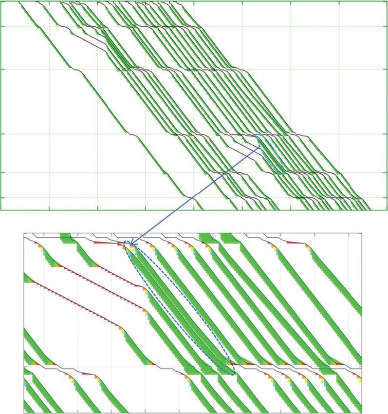
Journal of Advanced Transportation 11

 Time (h)
 9 9.5 10 10.5 11 11.5 12 12.5 13
 A

 B

 C
 Section

 D

 E

 F

 (a)
 11.4 11.5 11.6 11.7 11.8 11.9 12 12.1 12.2 12.3
 D

 E

 (b)
 Figure 11: Rescheduled timetable after the first-step computation.

proposed. If the computation time is 600 seconds, all of them keep the full-speed on the track sections as most as possible.
can be solved to get the best or optimal solutions within 5% In this way, it is not only that trains speed are reduced
optimality gap or less, and it is proved that the setting of according to the equipment of disturbance of speed limi-
disturbances listed in Figure 8 is the most difficult to be tation, but also the capacity of high-speed railway is max-
solved to get the best solution with 3% optimality gap under imized by the proposed method.
the given computation time. Regarding to the graphical description for the
 rescheduled timetable, solutions of the first-step and
5. Results Analysis second-step computation are given in Figure 11 and Fig-
 ure 12, respectively, where 20 trains’ running lines with five
Based on the data listed in Figure 8, solutions solved by the kinds of colors denote different speed levels. More precisely,
model are analysed in this part. First of all, we analysed the red, purple, yellow, blue, and green colors in running lines
speed level of the given trains, which are plotted in Figure 10. correspond to 1, 2, 3, 4, and 5 levels of train speed levels,
In detail, 20 broken lines represent speed levels (vertical axis) respectively (i.e., the detail refers Table 1). Furthermore,
of 20 trains along their routes (horizontal axis). It is noted there are two subpictures in both figures, where the upper
that the value of vertical axis is cycle number with 5 units figure is the whole rescheduled timetable and the bottom
divided by each horizontal line. In detail, the start value is picture presents a partial magnifying timetable denoted by
speed level 1 and the end is speed level 5 along the upward the blue cycle in the up figure. In this figure, there are two
direction in each cycle period. In terms of undulations of obvious parts denoting by two rectangle dotted boxes where
lines in railway station area, trains have to decelerate and trains’ speed reduced sharply due to speed limitations be-
accelerate their speed to aboard and alight passengers. tween stations B and C or stations D and E. It proved that the
Furthermore, the fluctuation (highlighted by the rectangular proposed model can control the speed of trains accurately to
shaded area) of lines no.2–4 and no.8–13 in the open track keep the safety of trains along railway track, though there are
area indicated the speed limitation effected by disturbances. two speed limitations with different geographical locations
In addition to above sections mentioned, all the lines can and time spans. Secondly, reordering trains and retiming

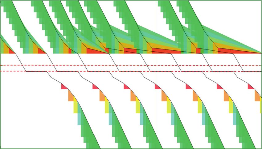
12 Journal of Advanced Transportation

 Time (h)
 9 9.5 10 10.5 11 11.5 12 12.5 13
 A

 B

 C
 Section

 D

 E

 F
 (a)
 11.4 11.5 11.6 11.7 11.8 11.9 12 12.1 12.2 12.3
 D

 E

 (b)
 Figure 12: Rescheduled timetables after the second-step computation.

trains are both executed to avoid some potential conflicts, train in each block section and its real-time speed level are
resulting from primary delay or infrastructure capacity. coordinate and the final solution is feasible enough. All in all,
 Comparison with Figures 11 and 12, the arrival or de- the proposed mathematical model and the solving method
parture times of trains at railway stations are almost the with the two-step algorithm are able to address train
same, but train orders and running times on sections are rescheduling problem under the influence of the
different, as well as conflicts between trains. To be specific, multidisturbances effectively.
there are some crosses or overlaps between trains’ running Concerning blockages of siding line in station C and
lines in the dash circles in Figure 11 and an obvious overlap station D, a case without siding line blockage is used as the
between trains in the bottom picture in Figure 11, consid- benchmark. Figure 13 shows negative influence of siding line
ering the crosses in open track area or overlaps reflect blockage, especially in arrival path areas in station C. It
conflicts caused by overpassing of trains in segment. This should be noted that two dash lines in Figure 13 represent
phenomenon must be forbidden in realistic railway oper- the siding lines in the geographical axis. Compared the
ation, as it means at least two trains occupy the same section timetable adjusted with siding line blockage (shown by
at the same time. Nevertheless, those two consecutive trains Figure 13) with that without siding line blockage (shown by
run on the segment with the maximum speed and minimum Figure 14), it is noticeable that some trains (in Figure 13)
headway distance in the bottom picture in Figure 12. As a have to wait outside station until the former train departure,
result, the solution computed by the first-step computation due to the limited capacity of available siding lines.
under the control of headway time interval and free-conflict Considering the shortage of capacity caused by siding
principle is not feasible and reliable sometimes. Given the line blockage in railway station, the waiting times of trains in
unreliability of the solution, the further measure should be front of station C related to those two cases are analysed in
carried out by the train scheduler or diver, if needed. Figure 15, where each column denotes waiting time of each
 With application of the strict headway space resched- train, i.e., the blue one relates to Figure 13 and the red one
uling rule in second-step solution, the running time of each relate to Figure 14. Compared with values of blue columns

Journal of Advanced Transportation 13

 Time (h)
 10.2 10.45

 C
 Section

 Figure 13: Timetable adjusted without siding line blockage in station C.

 Time (h)
 10.2 10.45

 C
 Section

 Figure 14: Timetable adjusted with siding line blockage in station C.

 300 and yellow columns, some of blue columns are much higher
 than yellow columns. To be specific, the waiting times of
 train 8th, 9th, 10th, and 14th in front of railway station are
 Waiting time (second)

 200 longer than that without blockage, and around 700 seconds
 are generated due to blockage of siding line in station C.

 100 6. Conclusions and Outlook
 Based on above content, the proposed MILP model is able to
 0 deal with the problem caused by primary delays, speed
 0 5 10 15 20 limitations, and blockages of siding lines at the same time,
 Index of trains and the characteristics of the quasi-moving block signalling
 Waiting time with blockage system are considered in the model, which make train
 Waiting time without blockage control possible along with train rescheduling. It succeeds in
 extending the alternative graph method mentioned by [18]
 Figure 15: Waiting time of each train in front of station C. and making rerouting possible along with retiming and

14 Journal of Advanced Transportation

reordering, although the signalling system of high-speed References
railway is more flexible and dynamic. Concerning above
experimental tests, we draw conclusions as follows: [1] F. Corman and L. Meng, “A review of online dynamic models
 and algorithms for railway traffic management,” IEEE
 (1) The proposed MILP model can deal with Transactions on Intelligent Transportation Systems, vol. 16,
 multidisturbances (i.e., multispeed limitations, no. 3, pp. 1274–1284, 2015.
 primary delay, and siding blockage) in one iteration [2] G. Cavone, M. Dotoli, N. Epicoco, and C. Seatzu, “A decision
 efficiently, by means of controlling train speed, making procedure for robust train rescheduling based on
 changing orders of trains, adjusting running times of Mixed Integer Linear Programming and Data Envelopment
 trains, and resetting arrival/departure paths in rail- Analysis,” Applied Mathematical Modelling, vol. 52,
 way station area, so it is a comprehensive mathe- pp. 255–273, 2017.
 [3] M. Dotoli, N. Epicoco, M. Falagario et al., “A decision support
 matical optimal method.
 system for real-time rescheduling of railways,” in Proceedings
 (2) The given two-step solution approach can accelerate of the 13th IEEE European control conference. (ECC 2014),
 the solving process by ignoring the conflicts between Strasbourg, France, June 2014.
 trains (i.e., overtaking) in segments, in the other [4] Y. Ye and J. Zhang, “Accident-oriented delay propagation in
 words, those constraints related to headway time high-speed railway network,” Journal of Transportation En-
 interval are considered in the railway station area gineering, Part A: Systems, vol. 146, no. 4, Article ID 04020011,
 firstly. The comparison with a benchmark algorithm 2020.
 is executed, and the priority of the proposed method [5] V. Cacchiani, D. Huisman, M. Kidd et al., “An overview of
 recovery models and algorithms for real-time railway
 is verified.
 rescheduling,” Transportation Research Part B: Methodolog-
 (3) Timetable adjusted by the mathematical model is ical, vol. 63, pp. 15–37, 2014.
 feasible and improved, where all conflicts are solved, [6] T. Dollevoet, D. Huisman, M. Schmidt, and A. Schöbel,
 based on a realistic high-speed railway line in China. “Delay management with rerouting of passengers,” Trans-
 Furthermore, all the trains are distributed with portation Science, vol. 46, no. 1, pp. 74–89, 2012.
 reasonable routes and given accurate speed levels [7] M. Dotoli, N. Epicoco, M. Falagario et al., “A real time traffic
 from the original to its destination. management model for regional railway network under
 disturbances,” in Proceedings of the 9th IEEE International
 There are some shortages remained to improve for future Conference on Automation Science and Engineering (CASE
research. First of all, the comparisons with current other 2013), Madison, WIUSA, August 2013.
methods related to train rescheduling will be under inves- [8] F. Corman, A. D’Ariano, A. D. Marra, D. Pacciarelli, and
tigation to study the effectiveness and generality of the M. Samà, “Integrating train scheduling and delay manage-
proposed method. Secondly, there are still a high-speed ment in real-time railway traffic control,” Transportation
railway network controlled by a quasi-moving block system Research Part E: Logistics and Transportation Review, vol. 105,
is still needed to explore by the proposed method, in terms of pp. 213–239, 2017.
 [9] W. Fang, S. Yang, and X. Yao, “A survey on problem models
dimension of research objective, N-track railway line, and so
 and solution approaches to rescheduling in railway networks,”
on. At last, concerning the disadvantage of commercial
 IEEE Transactions on Intelligent Transportation Systems,
solving software, a more powerful and efficient heuristic vol. 16, no. 6, pp. 2997–3016, 2015.
algorithm should be designed and applied to solve the [10] I. A. Hansen and J. Pachl, Railway Timetabling & Operations,
NP-hard problem, in order to meet the requirement of Eurailpress, Hamburg, Germany, 2014.
real-world railway operation. [11] S. Zhan, L. G. Kroon, L. P. Veelenturf, and J. C. Wagenaar,
 “Real-time high-speed train rescheduling in case of a complete
 blockage,” Transportation Research Part B: Methodological,
Data Availability vol. 78, no. 8, pp. 182–201, 2015.
Some or all data, models, or code that support the findings of [12] L. P. Veelenturf, M. P. Kidd, V. Cacchiani et al., “A railway
 timetable rescheduling approach for handling large-scale
this study are available from the corresponding author upon
 disruptions,” Transportation Science, vol. 50, no. 3,
reasonable request. pp. 841–862, 2015.
 [13] A. D’Ariano, D. Pacciarelli, and M. Pranzo, “A branch and
Conflicts of Interest bound algorithm for scheduling trains in a railway network,”
 European Journal of Operational Research, vol. 183, no. 2,
The authors declare that there are no conflicts of interest pp. 643–657, 2007.
regarding the publication of this paper. [14] F. Corman, A. D’Ariano, D. Pacciarelli, and M. Pranzo, “A
 tabu search algorithm for rerouting trains during rail oper-
 ations,” Transportation Research Part B: Methodological,
Acknowledgments vol. 44, no. 1, pp. 175–192, 2010.
 [15] M. Samà, A. D‫׳‬Ariano, F. Corman, and D. Pacciarelli, “A
This work was supported by the National Nature Science variable neighbourhood search for fast train scheduling and
Foundation of China (nos. 71801019 and 52072044), the routing during disturbed railway traffic situations,” Computers
Shannxi Science and Technology Project (nos. 2020JQ-390 & Operations Research, vol. 78, no. 2, pp. 480–499, 2017.
and 2020JQ-363), and the Open Project of State Key Lab- [16] M. Samà, C. Meloni, A. D’Ariano, and F. Corman, “A
oratory of Traction Power under grant no. TPL2108. multi-criteria decision support methodology for real-time

Journal of Advanced Transportation 15

 train scheduling,” Journal of Rail Transport Planning &
 Management, vol. 5, no. 3, pp. 146–162, 2015.
[17] M. Mazzarello and E. Ottaviani, “A traffic management
 system for real-time traffic optimisation in railways,” Trans-
 portation Research Part B: Methodological, vol. 41, no. 2,
 pp. 246–274, 2007.
[18] P. Xu, F. Corman, Q. Peng, and X. Luan, “A train rescheduling
 model integrating speed management during disruptions of
 high-speed traffic under a quasi-moving block system,”
 Transportation Research Part B: Methodological, vol. 104,
 pp. 638–666, 2017.
[19] P. Xu, F. Corman, Q. Peng, and X. Luan, “A timetable
 rescheduling approach and transition phases for high-speed
 railway traffic during disruptions,” Transportation Research
 Record: Journal of the Transportation Research Board,
 vol. 2607, no. 1, pp. 82–92, 2017.
[20] S. Long, L. Meng, Y. Wang et al., “A train rescheduling
 optimization model with considering the train control for a
 high-speed railway line under temporary speed restriction,” in
 Proceedings of the 2019 IEEE Intelligent Transportation Sys-
 tems Conference (ITSC), pp. 2809–2816, Auckland, New
 Zealand, October2019.
[21] X. Li, B. Shou, and D. Ralescu, “Train rescheduling with
 stochastic recovery time: a new track-backup approach,” IEEE
 Transactions on Systems, Man, and Cybernetics: Systems,
 vol. 44, no. 9, pp. 1216–1233, 2014.