Integrating Traffic Data and Model Predictive Control to Improve Fuel Economy
←
→
Page content transcription
If your browser does not render page correctly, please read the page content below
Integrating Traffic Data and Model Predictive Control to Improve Fuel Economy

                                      Nicholas J. Kohut,* Professor J. Karl Hedrick,**
                                              Professor Francesco Borrelli.***

                 *Mechanical Engineering Department, University of California-Berkeley, Berkeley, CA 94720
                                 USA (Tel: 510-642-6933; e-mail: kohut@ berkeley.edu).
                ** Mechanical Engineering Department, University of California-Berkeley, Berkeley, CA 94720
                               USA (Tel: 510-642-2482; e-mail: khedrick@me.berkeley.edu).
               *** Mechanical Engineering Department, University of California-Berkeley, Berkeley, CA 94720
                               USA (Tel: 510-643-3871; e-mail: fborrelli@me.berkeley.edu)

          Abstract: This paper presents a method for increasing fuel economy using traffic data and a model
          predictive controller. Using knowledge of the traffic ahead, a vehicle can react to changes in traffic
          density or speed before they happen, increasing the efficiency of a trip and providing valuable
          information to the driver. In particular, the traffic information is used to determine a time-varying
          velocity envelope that the vehicle must satisfy. Then, a vehicle model is used to compute the vehicle
          speed profile that minimizes fuel use and satisfies the velocity constraints. Simulation results show the
          feasibility of the proposed approach on a passenger vehicle with minor hardware modifications required
          for its implementation.
          Keywords: Intelligent Transportation Systems, Model Predictive Control, Intelligent Vehicles, Engine
          Control, Adaptive Cruise Control

                                                                  In our first work [5] we have shown the early development of
1. INTRODUCTION
                                                                  the longitudinal and fuel models, along with preliminary
Today’s world sees an ever-increasing demand for more             simulative results applied to the EPA Highway driving cycle.
environmental and fuel-efficient technologies. These              This work expands on that by performing a closer
technologies often involve significant hardware modifications     examination of the models involved, and using actual driving
that improve the overall efficiency of a vehicle, but do not      data to test the performance of the controller, with
address how to drive a vehicle in the most efficient manner.      interpretation of these results.
Simply by driving a vehicle more efficiently, fuel economy
can be improved and emissions can be reduced today, on            The paper is structured as follows. First, the vehicle and fuel
today’s vehicles, at little to no cost.                           consumption models are presented. These models must be
                                                                  descriptive enough to accurately represent the longitudinal
Past work has shown promising results in this area.               dynamics of the vehicle and the vehicle’s fuel use, but also
Simulative results have predicted that less than 60 seconds of    simple enough to be used in real-time control, where a
preview time of traffic conditions can yield fuel economy         complex model would pose an insurmountable computational
improvement equal to that of a hybrid vehicle using a             burden. Then, an overview of the data sources and Model
conventional powertrain, without the heavy investment in          Predictive Control (MPC) scheme are presented.
new powertrain technology. Longer preview times of around
180 seconds have been shown to reduce fuel consumption by         Model Predictive Control theory [8] is an online optimization
up to 33% [5]. Other experimental work has shown 3.5%             method that can incorporate knowledge of future conditions
improvement in fuel economy without an increase in trip time      such as road grade changes and traffic flow variations as well
[4].                                                              as hard constraints on engine control variables. Recently, this
                                                                  method has been receiving a great deal of attention due to the
This paper formulates a predictive control problem in order to    speed and memory capability of modern microprocessors.
improve fuel economy by controlling the speed of the vehicle
through the Adaptive Cruise Control, while fulfilling various     MPC uses a model of the plant to predict the future evolution
constraints related to traffic and driver comfort. At each step   of the system. Based on this prediction, at each step a
information about the surrounding traffic is assumed to be        performance index is optimized subject to linear and
known over a finite horizon, and a receding horizon               nonlinear constraints with respect to a sequence of future
controller computes the engine torques required to navigate       inputs. The first of these optimal moves is the control action
traffic and minimize fuel use on a public highway.                applied to the plant at step k. At step k+1, a new optimization
                                                                  problem is solved over a shifted prediction horizon.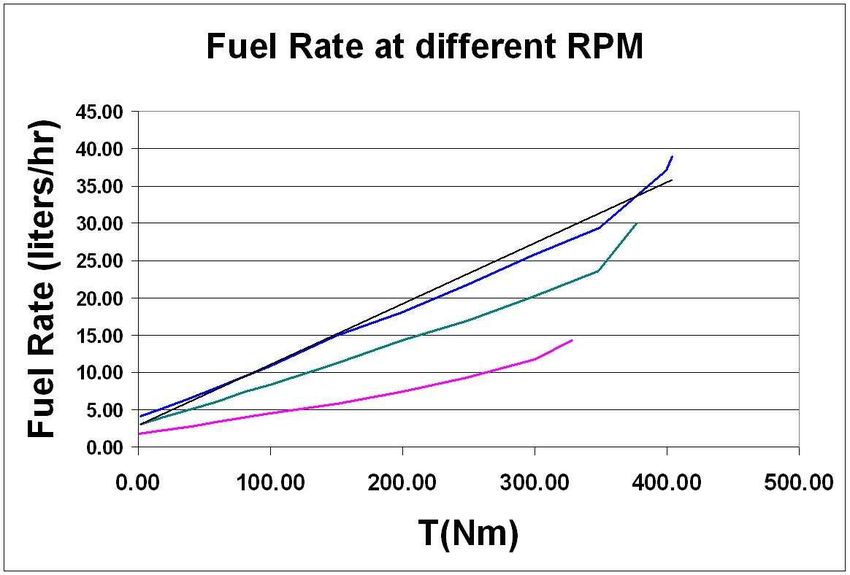
2.1 Longitudinal Model
Advances in both theory and computing systems have
expanded the range of applications where real-time MPC can                    The discrete longitudinal model is based on the
be applied [9]. Yet, for a wide class of “fast” applications the     principle that the energy at the next step is a function of the
computational burden of Nonlinear MPC is still a serious             energy at the current step plus the change in energy, caused
barrier for its implementation [1]. The paper concludes with         by engine torque and air and road drag.
some simulative results and their implementation.
                                                                     1                   1          1
1.1 Approach                                                           mv 2 ( k + 1) = mv 2 ( k ) − ρ ( C a )( ∆ s ) v 2 ( k )
                                                                     2                   2          2                          (1)
                                                                       R∆s
Traffic data is most available and reliable on highways. In          +       (η )T ( k ) − µ mg ∆ s
addition, highway traffic is more predictable, and does not             r
include stop signs, stop lights, or other confounding factors.
Due to these advantages, the proposed system is intended for
highway use only, where adaptive cruise control can be used          We use      s (k ) as the independent variable, representing
to regulate the speed of the vehicle.                                position, and a fixed step size of ∆s = s ( k + 1) − s ( k ) for
We make use of a vehicle model that relates engine torque to         all k. v(k ) is the velocity of the vehicle at position s (k ) ,
vehicle speed and fuel consumption. Since the adaptive cruise        Ca is the coefficient of drag multiplied by the car’s frontal
control is used to control the vehicle, no low-level engine          area, m is the effective mass of the vehicle, r is the rolling
dynamics must be modelled. It is assumed that the engine             radius of the tire, R is the ratio of wheel to engine speed, and
will provide the torque requested of the ACC instantly. Real-         g is the gravitational constant. R is assumed to be constant
time traffic data comes primarily from the California                for this formulation.   η   is the driveline efficiency, which is
Freeway Performance Measurement System, or PeMS [7].
PeMS provides average traffic speed and density at a                 considered constant here. T ( k ) is the torque output of the
resolution of 0.3 to 3 miles every five minutes. This distance       engine at position s ( k ) . µ is the friction coefficient
interval depends on the nature of the highway. If there are no       associated with the rolling resistance; it is assumed to be
exits on a stretch of highway (e.g. a bridge) only one loop          constant. It is assumed the tire slip is small, and is not taken
will be used to measure traffic, regardless of the length of the     into account.
link. Areas with more exits carry more loops, preserving
accuracy. In addition, the use of probe data is anticipated.         Such an oversimplified model is used to insure the
Probe vehicles are vehicles that carry special cell phones that      optimization problem solved at each step is tractable and can
are able to communicate their position and velocity in real-         be solved in real-time on current automotive Electronic
time. If there were probe vehicles near the controlled vehicle,      Control Units (ECUs). The model parameter can be identified
this would provide a high fidelity measure of the traffic            and even adjusted in real time in order to better fit the
directly surrounding it.                                             measurements. The figure below shows a simple comparison
                                                                     between experimental data and model predictions with no
Model Predictive Control is employed to compute an optimal           tuning of model parameters.
engine torque every forty meters, using vehicle states and
traffic measurements as inputs. When the models, data, and
control strategy are combined, the optimal torque can be sent
to the vehicle’s ACC to drive the car in the most efficient
way possible. The system can be easily deactivated by the
driver or by the ACC if the vehicle detects another car too
close. In addition, because the controller requires an accurate
representation of the traffic in front of the vehicle, this can be
displayed to the driver, showing what to expect ahead.

2. MODELING
Two models are used for this work. A longitudinal model
based on the work-energy principle is used to predict how the
vehicle will travel down the road given its speed, torque, and
gear. The formulation of this model is linear with respect to
its state (vehicle velocity squared) and its input (torque). A       Fig. 1: Model Correlation with Audi A8L controlled by ACC
nonlinear fuel model is used to predict how much fuel is
consumed by the vehicle based on speed, torque, and gear.
These two models allow the controller to accurately predict          2.2 Fuel Model
vehicle speed and fuel consumption.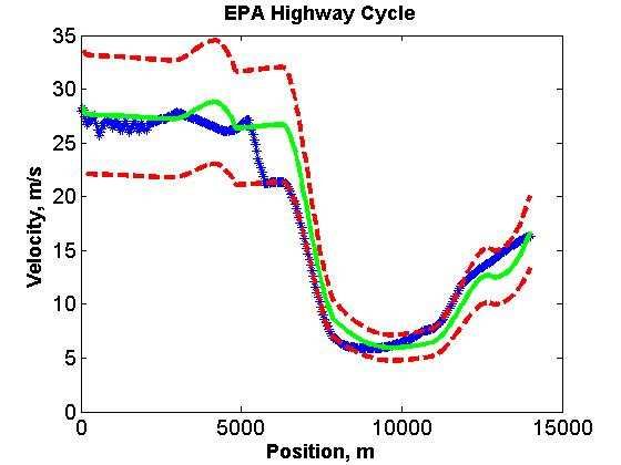
The fuel model has been developed from static dynamometer
test data. This data involves measuring the fuel consumption
at various values of constant torque and rpm.
Fig. 4: c2 varies linearly with engine speed
The resulting equation is
•
f (k) = c(ω e2 (k)) + d(T(k))(ω e (k)) (3)
where ω e ( k ) is the engine speed at position s (k ) and c and
Fig. 2: Fuel Use for various RPM and Torque d are constants. Since we are interested in the total fuel use
and not simply the rate, we multiply the fuel rate at position
The figure above shows a normalized fuel consumption for s (k ) by the time it takes to reach position s(k + 1) . This
various values of constant RPM while the torque is varied. A
time can be found by dividing the step length by the velocity
linear fit was made for each line (not all lines are shown here
for clarity) to determine the best approximation of this data. at position s (k ) :
The average R2 value for these fits is 0.9769, with a worst R2 ∆s
of 0.9708. This leads to the following equation t(k) = (4) (1
v(k)
•
f (k) = c1 + c 2T(k) (2) In order to use the model states, the engine speed is converted
to vehicle speed through the ratio of engine to wheel speed
• and tire radius:
where c1 and c 2 are constants and f (k) is the fuel rate at
•
v(k)
position s (k ) . We remark that f is a symbol. In order to ω e (k) = R (5)
account for engine speed the coefficients c1 and c 2 are
r
parameterized as functions of engine speed. This gives the final fuel model
R 2 R
f (k) = c(v(k)) + d(T(k)) ∆s (6)
r r
3. CONTROLS
3.1 Data Sources
To gather information about traffic around the vehicle, two
major data sources are used. The first source is used to
determine the state of traffic far from the vehicle. This comes
Fig. 3: c1 varies linearly with engine speed squared from the California Freeway Performance Measurement
System, or PeMS. PeMS uses loop detectors embedded in
When c1 and c 2 are plotted against engine speed squared, a California freeways to measure the speed and density of
traffic every 30 seconds. This is the aggregated into lane-by-
linear fit is very satisfactory, as shown in Figure 3 and 4.
lane data every 5 minutes. PeMS loops are positioned
approximately every 0.3 to 3 miles along the road [6].
PeMS allows an accurate picture of the traffic ahead of the
vehicle, but lacks the necessary resolution to be useful near
the vehicle. This requires a different set of data. To create an
accurate picture of the traffic directly around the vehicle,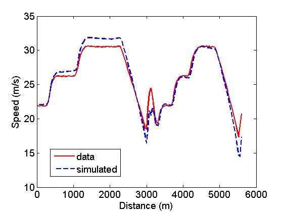
other “probe vehicles” are used. These are cars that have been where T(k) is the set of torques over the finite horizon of
equipped with a cell phone that can broadcast the car’s 2
position and velocity. Once this data is available and size n at position s (k ) . Similarly, v (k) is the set of the
widespread, information about traffic flow almost anywhere velocities squared over the horizon. The function to be
can be easily used. At this point usage is fairly low, but for minimized is the fuel use over the horizon. The first
the purposes of this project it is assumed penetration will constraint represents a bound on the torque, while the second
increase in the future and that this will be a viable data constraint is a linear constraint restricting the vehicle’s
source. velocity (a linear function of torque). The final constraint
restricts the time spent on the horizon, a nonlinear function of
When these data sets are combined, they create a picture of torque. This optimization problem is solved at every step
the behavior of the traffic ahead of the vehicle. To quantify using the software package NPSOL [3].).
this, a velocity profile is created of the expected traffic speed,
which is then used in the controller. Combining the short The cost function to be minimized is the sum of the fuel use
distance probe data and long distance PeMS data creates the at each step over the horizon.
profile seen below.
N
J = ∑ f (k + i) (8)
i=1
The bounds on the torque limit the maximum acceleration of
the vehicle, for purposes of driver comfort. This is generally
set so that the maximum acceleration is always below 0.4 g’s,
in acceleration or braking. The linear constraints restrict the
velocity the vehicle can travel. This is necessary in traffic,
where, if traffic is flowing at 60 mph, speeds of 90 mph may
be undesirable (and illegal), but so may be speeds of 30 mph.
Hence, an upper and lower limit on speed is placed on the
vehicle for safety reasons based on the traffic around it. This
constraint is realized as
LSC 2v avg
2
(k) ≤ v 2 (k) ≤ USC 2v avg
2
(k) (9)
Fig. 5: An Example Velocity Profile where LSC is the lower speed constraint factor, and USC is
3.2 MPC the upper speed constraint factor.
The data discussed above is used to design a feedback control The final constraint faced by the controller is a constraint on
scheme to control the vehicle and reduce fuel consumption. time. To simply save fuel, going as slow as possible is often
Every second, the velocity profile determined by the (though not always) the optimal choice. This strategy
incoming data is fed to the controller, along with the current provides trivial results and little true benefit to the driver. To
vehicle speed. Using this information, an optimal torque is insure the trip is completed in a timely manner, an upper
determined and commanded to the ACC. constraint is placed on the time. Here we consider the time
over the entire horizon in our constraint, which we will call
3.3 Problem Formulation τ (k) .
MPC is used to predict the future use of fuel for various N
choices of future torques. This fuel use is minimized, subject τ (k) = ∑ t(k + i) (10)
to constraints on maximum torque, vehicle velocity, and i=1
travel time. To minimize the fuel use subject to these
constraints, the following nonlinear programming problem It would seem best to constrain the trip time to a given value,
must be solved at each step: for example, to travel from point A to point B in less than 20
minutes. In practice though, this is difficult. Predicting what
min J(v 2 (k),T(k)) traffic conditions will be far ahead is unreliable, and the
T (k )∈ℜn computing power required to process an entire trip is not
T(k) available. It would also be advantageous for the driver to
(7) choose to what degree he or she would like to balance the trip
subject to lb ≤ AT(k) ≤ ub time and fuel economy. The solution chosen allows this.
c(T(k))
To determine the balance of fuel economy and trip time, the
control system uses the model propagation and the velocity
constraints to determine the shortest time path and the longest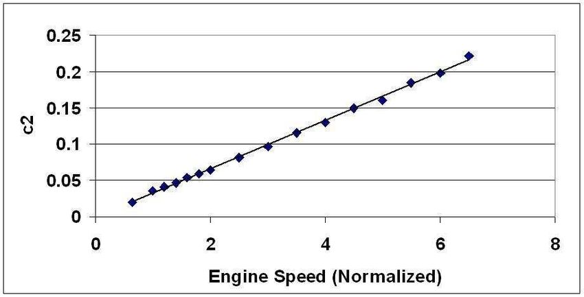
time path over a horizon. The driver supplies a “fuel rating,” vehicle travels slowly relative to the traffic when the average
κ , at the outset of the trip. This is a number from zero to speed is high, and relatively quickly when the average speed
100. Then the time spent to traverse the horizon is is low. To balance fuel use and trip time, it makes sense to
constrained to a value between the shortest time and least fuel slow down a bit at high speeds, when fuel consumption is
time according to the rating. high due to air drag, and make up for lost time by going a bit
κ faster at low speeds, where the air drag penalty for doing so is
τ (k) ≤ τ min (k) − (τ min (k) − τ max (k)) (11) much lower. (29)
100
4.1 Optimal Horizon Length
Once the cost function and all the constraints have been
established, a set of optimal torques can be established. At
Picking the horizon length is important for a problem of this
this point, the first optimal torque is applied, the horizon is
nature. A long horizon generally offers an advantage in
re-established and re-evaluated, and the whole process
predictive control, because more data can be taken into
repeats until the trip ends.
account. However, if this data is unreliable, it may not be
useful. Additionally, a long horizon means the solution takes
4. RESULTS
much longer to compute, which can be critical in a real-time
application such as this one.
To test this formulation, a trip was taken from Palo Alto, to
San Jose, California, while recording average traffic speed.
Due to these considerations, it is desired to use a horizon that
Using this data, simulations were run to determine how much
will be long enough to effectively improve fuel economy,
fuel could have been saved if different driving choices had
while being short enough to process in real-time and provide
been made. The vehicle has a horizon length of 2000 meters.
reliable data. Testing for an ideal horizon can be difficult,
This means the traffic ahead of the vehicle up to 2000 meters
because various traffic situations will have different optimal
at any time is assumed to be known.
horizon lengths. This optimal length will be dependent on the
traffic in front of the vehicle, and how quickly and to what
degree the traffic speed changes. In the presented results we
have chosen to use one trip as a benchmark, find the optimal
horizon, and then use this as the horizon for all trips. Clearly
the option is to change the horizon length in real-time as a
function of environment and traffic conditions.
To find a suitable trip to determine the optimal horizon
length, the EPA Highway fuel economy cycle was used as a
baseline. This cycle is designed to represent a range of traffic
conditions and will be what the vehicle is judged on in the
marketplace for fuel economy.
A simulation similar to the results in Section 4 was run to
determine the best horizon length. Again, the prescribed
speed was used as a baseline, while the vehicle was
constrained to travel no more than 20% faster or slower than
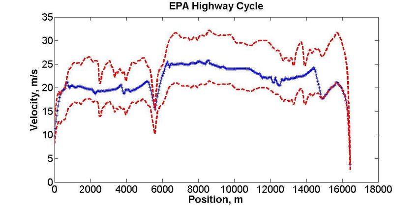
Fig. 6: A simulation run the baseline speed at all times. Horizon lengths of 1200,
1600, 2000, 3000, 4000, and 5000 meters were tested.
The above graph shows the results of the simulation. The x-
axis represents the distance along the trip while the y-axis
represents the vehicle speed. The solid line represents the
average traffic velocity, which serves as a baseline for
comparison. The dashed lines represent the velocity
constraints. The velocity must stay in between these lines at
all times. Finally, the line of asterisks recommends the path
that should be taken by the car in order to balance trip time
and fuel economy best. This path takes the same amount of
time to complete as the green path, but uses 5.4% less fuel. It
is likely that the controller chooses this path for a few
reasons. One is that if the vehicle is slowing down, but must
speed up again in the future, it is advantageous to not slow Fig. 7: EPA Highway Cycle Results
down all the way, to reduce the amount of acceleration
needed to keep up with traffic. This is seen between 8000 and The figure above shows the results of the 2000 meter horizon
12000 meters on the trip. Similarly, at around 4000 meters, simulation. In this case, 7.2% less fuel is used compared to
the vehicle sees a drop in speed and decides to slow down to the baseline case, while the trip takes 2.9% longer. The
preserve fuel. Another advantage of this path is that the results of each horizon length are shown in the table below.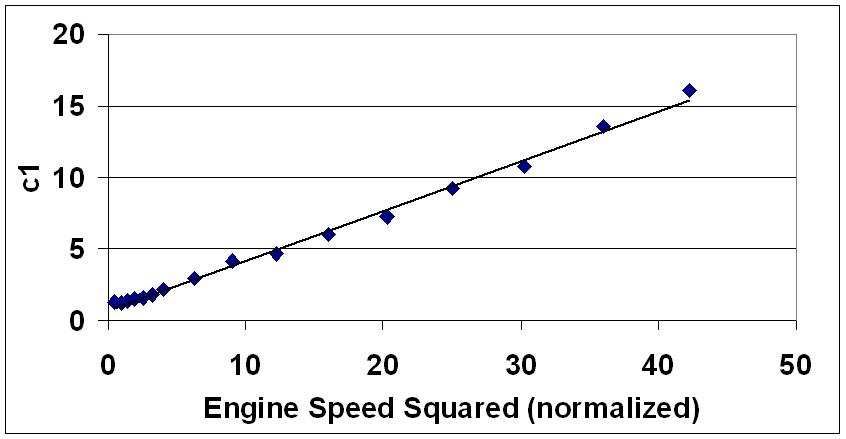
P. Falcone, F. Borrelli, J. Asgari, H. E. Tseng, and D. Hrovat,
Table 1: Fuel and Time savings vs. Horizon Length                       “Predictive active steering control for autonomous
                                                                        vehicle systems,” Accepted for publication in IEEE
    Horizon Length (m) Fuel Saved (%) Time Saved (%)
                    1200            5.2           -2.1                  Trans. on Control System Technology, 2006.
                    1600            6.4           -2.2
                    2000            7.2           -2.9              Phillip E. Gill, Walter Maurray, Michael Sanders, Margaret
                    3000            8.7           -4.6
                    4000            9.6           -5.8                   Wright, “User’s Guide for NPSOL 5.0: A FORTRAN
                    5000           10.3           -6.7                   Package for Nonlinear Programming”, Technical Report
                                                                         SOL 86-1, July 1998
Positive percentages indicate improvements (less fuel or less
time) while negative percentages indicate more fuel or time         E. Hellstrom, M. Ivarsson, J. Aslund, L, Nielsen, “Look
use. In this case, as the horizon length increases, the fuel            Ahead Control for Heavy Trucks to Minimize Trip Time
savings increase as well. However, the trip time increases as           and Fuel Consumption” Fifth IFAC Symposium on
the horizon length goes up. It should be kept in mind that the          Advances in Automotive Control, August 20-22, 2007,
fuel use is minimized subject to constraints, while the trip            Aptos, California.
time is constrained over the horizon to a certain value. This
means that increasing horizon length gives more information         N. Kohut, F. Borrelli, K. Hedrick (2008). “Utilization of
to the controller which it can use to minimize fuel use, but            Intelligent Transport Systems Information to Increase
since the torque and horizon are updated every step, there is           Fuel Economy through Engine Control.” 15th World
no guarantee the total time will improve. To decide which of            Congress on Intelligent Transport Systems, November
these situations is best, the percentage improvements for the           16-20, 2008, New York City, New York.
fuel and time were added to create a “performance index.”           Chris Manzie, Harry Watson, Saman Halgamuge, “Fuel
                                                                        Economy Improvements for Urban Driving: Hybrid vs.
                                                                        Intelligent Vehicles”, Transportation Research Part C,
                                                                        pp. 1-16, 2007
                                                                    California Freeway Performance Measurement System,
                                                                        http://pems.eecs.berkeley.edu
                                                                    D.Q. Mayne, J.B. Rawlings, C.V. Rao, P.O.M. Scokaert,
                                                                       “Constrained Model Predictive Control: Stability and
                                                                       Optimality”, Automatica 36, November 1999, p. 789-814
                                                                    V. M. Zavala, C. D. Laird, and L. T. Biegler. Fast solvers and
Fig. 8: Performance Index peaks at 2000 meters                          rigorous models: Can both be accomodated in nmpc?
                                                                        IFAC Workshop on Nonlinear Model Predictive Control
It is clear here that 2000 meters is the best choice, and this is       for Fast Systems, plenary talk, 2006.
the horizon used for all simulations.

                      5. CONCLUSION

This work displays promising simulations that show
reductions in fuel economy with little to no addition of
hardware to the vehicle. A model has been developed that
successfully reproduces vehicle behavior and can be used in a
real-time control scheme. Model Predictive Control is used to
minimize fuel use while maintaining realistic vehicle speeds
and trip times. This leads to a fuel savings of 5 to 7 % for a
trip time that changes 3% or less. The strategies presented
here are close to implementation and could show an almost
immediate affect on fuel economy for cars with access to
traffic data similar to that used in our work.

REFERENCES
P. Falcone, F. Borrelli, J. Asgari, H. E. Tseng, and D. Hrovat,
    “A Hierarchical Model Predictive Control Framework
    for Autonomous Ground Vehicles,” American Control
    Conference, June 11-13, 2008, Seattle, Washington.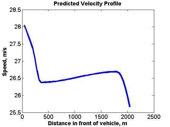
You can also read