Linking rain into ice microphysics across the melting layer in stratiform rain: a closure study
←
→
Page content transcription
If your browser does not render page correctly, please read the page content below

Atmos. Meas. Tech., 14, 511–529, 2021
https://doi.org/10.5194/amt-14-511-2021
© Author(s) 2021. This work is distributed under
the Creative Commons Attribution 4.0 License.

Linking rain into ice microphysics across the melting layer in
stratiform rain: a closure study
Kamil Mróz1 , Alessandro Battaglia2,3 , Stefan Kneifel4 , Leonie von Terzi4 , Markus Karrer4 , and Davide Ori4
1 National  Centre for Earth Observation, University of Leicester, Leicester, UK
2 Earth  Observation Science, Department of Physics and Astronomy, University of Leicester, Leicester, UK
3 Department of Environmental, Land and Infrastructure Engineering (DIATI), Politecnico of Turin, Turin, Italy
4 Institute for Geophysics and Meteorology, University of Cologne, Cologne, Germany

Correspondence: Kamil Mróz (kamil.mroz@le.ac.uk)

Received: 6 July 2020 – Discussion started: 22 July 2020
Revised: 19 November 2020 – Accepted: 11 December 2020 – Published: 25 January 2021

Abstract. This study investigates the link between rain and      through the melting zone is well preserved except the periods
ice microphysics across the melting layer in stratiform rain     of intense riming where the precipitation rates were higher
systems using measurements from vertically pointing multi-       in rain than in the ice above. This is potentially due to ad-
frequency Doppler radars. A novel methodology to exam-           ditional condensation within the melting zone in correspon-
ine the variability of the precipitation rate and the mass-      dence to high relative humidity and collision and coalescence
weighted melted diameter (Dm ) across the melting region is      with the cloud droplets whose occurrence is ubiquitous with
proposed and applied to a 6 h long case study, observed dur-     riming. It is shown that the mean mass-weighted diameter
ing the TRIPEx-pol field campaign at the Jülich Observatory      of ice is strongly related to the characteristic size of the un-
for Cloud Evolution Core Facility and covering a gamut of        derlying rain except the period of extreme aggregation where
ice microphysical processes. The methodology is based on         breakup of melting snowflakes significantly reduces Dm . The
an optimal estimation (OE) retrieval of particle size distri-    proposed methodology can be applied to long-term observa-
butions (PSDs) and dynamics (turbulence and vertical mo-         tions to advance our knowledge of the processes occurring
tions) from observed multi-frequency radar Doppler spectra       across the melting region; this can then be used to improve
applied both above and below the melting layer. First, the       assumptions underpinning spaceborne radar precipitation re-
retrieval is applied in the rain region; based on a one-to-      trievals.
one conversion of raindrops into snowflakes, the retrieved
drop size distributions (DSDs) are propagated upward to
provide the mass-flux-preserving PSDs of snow. These ice
PSDs are used to simulate radar reflectivities above the melt-   1   Introduction
ing layer for different snow models and they are evaluated
for a consistency with the actual radar measurements. Sec-       The accurate quantification of ice cloud macro-physical
ond, the OE snow retrieval where Doppler spectra are sim-        (height, thickness) and micro-physical properties (character-
ulated based on different snow models, which consistently        istic particle size and shape, mass content, and number con-
compute fall speeds and electromagnetic properties, is per-      centration) is paramount for understanding the current state
formed. The results corresponding to the best-matching mod-      of Earth’s hydrological cycle and energy budget and to im-
els are then used to estimate snow fluxes and Dm , which are     prove the representation of clouds for climate model pre-
directly compared to the corresponding rain quantities. For      dictions (Stephens, 2005; Tao et al., 2010). Macro-physical
the case study, the total accumulation of rain (2.30 mm) and     properties can be well captured by active remote sensing
the melted equivalent accumulation of snow (1.93 mm) show        instruments (Stephens et al., 2018); on the other hand, the
a 19 % difference. The analysis suggests that the mass flux      characterization of ice microphysics remains one of the most
                                                                 challenging problems (Heymsfield et al., 2018) because of

Published by Copernicus Publications on behalf of the European Geosciences Union.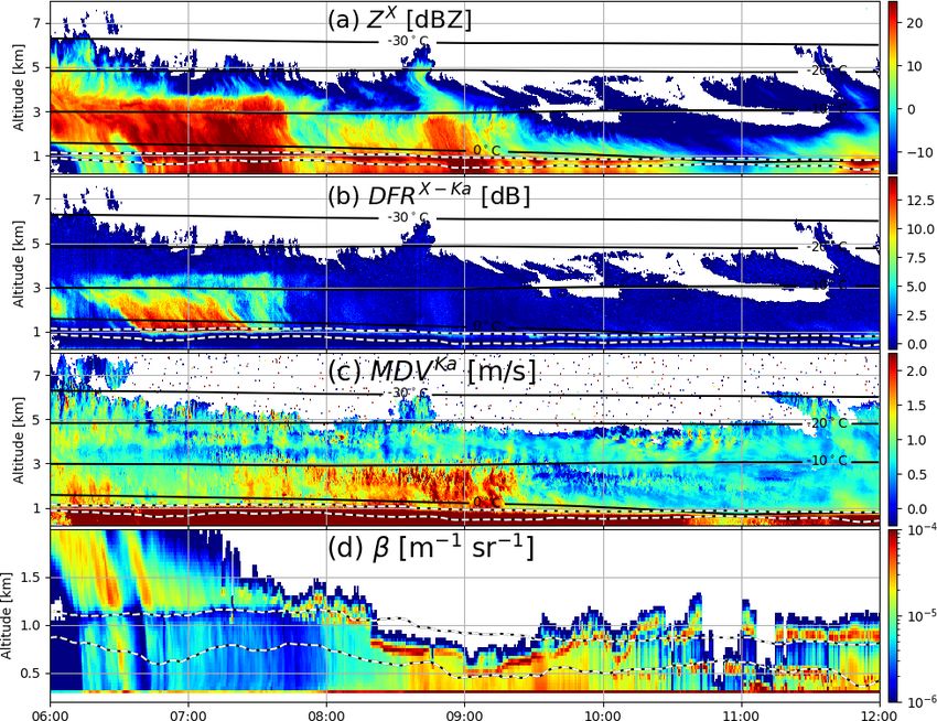
512                                                                                       K. Mróz et al.: Spectra closure study

the substantial number of assumptions about the particle size       surement (ARM) site have shown large signatures of differ-
distribution (PSD) and the particle “habit” type (such as den-      ential reflectivity ZDR from plate-like crystals (Oue et al.,
drites, columns, rosettes, aggregates or rimed particles) re-       2015a) whilst analysis of linear depolarization ratio (LDR)
quired in remote sensing techniques. While the characteriza-        in the spectral domain enabled the identification of columnar
tion of small ice crystals is particularly relevant for detailing   ice crystal growth originating in liquid-cloud layers through
the radiative effects of high ice clouds, understanding pro-        secondary ice production (Oue et al., 2015b).
cesses like aggregation, riming and deposition is essential for        Whilst several studies have looked at the microphysical
accurately modeling precipitation.                                  processes occurring within the melting layer (Drummond
   The study of stratiform precipitation encompasses the in-        et al., 1996) and at the link between microphysical processes
vestigation of such processes “within the context of relatively     in snow above the freezing level and within the melting
gentle upward air motion” (Houze, 1997). Stratiform precipi-        layer (Zawadzki et al., 2005; Li et al., 2020, and references
tation accounts for (> 85 %) 73 % of the area covered by rain       therein), less attention has been paid to the analysis of quan-
and (> 77 %) 40 % of the total rain amount across the (mid-         titative relationships between ice microphysics just above the
latitudes) tropics (Daniel Watters, personal communication,         freezing level and rain microphysics just below the melting
2020; Schumacher and Houze, 2003). Stratiform rain can be           layer. This investigation can contribute to a holistic under-
identified well in radar data displays by a bright band, i.e., a    standing of the chain of processes occurring in the cloud that
pronounced layer of enhanced reflectivity corresponding to          lead to precipitation at the ground, which is key for model
the melting layer (Fabry and Zawadzki, 1995).                       development but which may also help in better constraining
   In the past decade, several remote-sensing studies char-         full-column remote sensing retrievals, e.g. those applicable
acterized micro-physical processes occurring in the ice (e.g.       to spaceborne radars like GPM, CloudSat and EarthCARE
Kneifel et al., 2011, 2015; Kalesse et al., 2016; Leinonen and      (Battaglia et al., 2020a) but also for improving quantitative
Moisseev, 2015; Oue et al., 2015b; Stein et al., 2015; Ma-          precipitation estimation (QPE) from ground-based radar ob-
son et al., 2018; Tridon et al., 2019) and rain part of clouds      servations (Gatlin et al., 2018).
(e.g. Williams, 2016; Tridon et al., 2017b). The commonality           A common assumption used across the melting layer is
of all these studies resides in exploiting ground-based active      the conservation of water mass flux (e.g. Drummond et al.,
(radar and lidar) and passive (microwave radiometer) instru-        1996) which follows from assuming a stationary process
ments in a synergistic manner, with multi-frequency and/or          and neglecting evaporation and condensation effects. The
Doppler and/or polarimetric radars constituting the backbone        mass flux continuity assumption underpins several space-
of the observing system. Multi-frequency methods (Battaglia         borne radar stratiform precipitation retrieval algorithms (e.g.
et al., 2020a) rely on the fact that, when the wavelength of        Haynes et al., 2009; Mason et al., 2017); in other retrievals
the radars becomes comparable to the size of the particles          where this constraint is not adopted, large discontinuities be-
being probed (“non-Rayleigh” regime), the measured reflec-          tween mass fluxes above and just below the melting layer
tivity changes (typically decreases) relative to the Rayleigh       (Fig. 10 in Heymsfield et al., 2018) are reported. This incon-
regime, because the backscattered waves from different parts        sistency between rain and snow mass fluxes pinpoints at the
of the scatterer interfere (in a typically destructive way) with    presence of some underlying issues in the snow retrievals,
one another. Previous studies have demonstrated that dual-          which are more uncertain (Heymsfield et al., 2018; Tridon
and triple-frequency radar observations can provide addi-           et al., 2019).
tional information on bulk density and the characteristic size         In addition to water mass flux continuity, several studies
of the ice PSD (Kneifel et al., 2015; Battaglia et al., 2020b).     (Szyrmer and Zawadzki, 1999; Matrosov, 2008) further as-
Doppler (full spectral) information allows separation of par-       sume a one-to-one correspondence between the snowflake
ticles with different terminal velocities. While this informa-      falling across the zero isotherm and the raindrop into which it
tion is more valuable in rain than in ice, since the velocity       melts (i.e., aggregation and breakup are neglected). We will
of raindrops is unambiguously related to their mass and size        refer to this as to the “melting-only steady-state” (“MOSS”)
(which is not true of snow), Doppler spectra allow the de-          assumption. Under this condition, there is a unique corre-
tection of the presence of riming, which leads to an acceler-       spondence between the drop size distribution (DSD) of rain-
ation of the particle fall velocities above the typical 1 m s−1     drops and the PSD of snowflakes. If true this property could
observed for snow aggregate (Kneifel and Moisseev, 2020).           indeed be used to constrain the retrieval of hydrometeor ver-
The increasing terminal velocity of rimed particles causes          tical profiles in stratiform precipitation like done in Haynes
the spectra to be first skewed, and, at larger riming, to be-       et al. (2009) for the CloudSat spaceborne radar.
come bi-modal (Zawadzki et al., 2001; Kalesse et al., 2016;            The goal of this study is to propose a methodology ap-
Vogel and Fabry, 2018). Polarimetric radar observations are         plicable to multi-frequency Doppler polarimetric vertically
particularly sensitive to depositional growth in temperature        pointing radar measurements which enables the investigation
regions which favor growth of non-spherical particle shapes         of the relationship between the microphysics of snow and of
(e.g. needles, plates, dendrites). Observations obtained at the     the rain produced via melting. Some of the science questions
North Slope of Alaska (NSA) Atmospheric Radiation Mea-              (SQ) that will be addressed in this paper are as follows.

Atmos. Meas. Tech., 14, 511–529, 2021                                                 https://doi.org/10.5194/amt-14-511-2021

K. Mróz et al.: Spectra closure study                                                                                            513

SQ1. What is the relationship between mass fluxes above and           0.1◦ , which is expected to ensure a very high quality of the
     below the melting layer? How much does it deviate                multi-frequency measurements.
     from the commonly used constant mass flux assump-
     tion?                                                            2.2   The 24 November 2018 case study

SQ2. Can information about rain microphysics and DSD (e.g.            The focus of our analysis is on a short time period (06:00–
     about the mean characteristic size) be used to better con-       12:00 UTC) during a rain event on 24 November 2018. Se-
     strain the microphysical properties and PSD of the snow          lected radar measurements for this event are depicted in
     above?                                                           Fig. 1. The top and bottom of the melting layer have been
                                                                      derived with the linear depolarization ratio (LDR) from the
SQ3. Are there specific ice cloud regimes (e.g. dominated by          Ka-band radar following the method described in Devisetty
     aggregation or riming) where the MOSS or the flux-               et al. (2019). This approach is based on a very strong bright
     continuity assumptions are more likely violated?                 band signature in the LDR data in correspondence to the
                                                                      melting regardless of the rainfall intensity. In this study, the
    The paper is organized as follows: the dataset and the pro-       inflection points around the LDR peak are used as the top
 posed methodology are presented in Sects. 2 and 3, respec-           and the bottom of the melting zone. Over the presented time
 tively; Sect. 4 discusses the results for a case study in relation   period, the altitude of the 0 ◦ C isotherm was very stable and
 to the science questions; conclusions are drawn in Sect. 5.          decreased by only 300 m from 1.1 km at 06:00 UTC to 0.8 km
                                                                      at 12:00 UTC. Radar reflectivity data below the bright band
                                                                      indicate two intervals of intensified rainfall: the first period
 2     Dataset                                                        is from 06:45 to 07:45 UTC with the peak at 07:30 UTC and
                                                                      a shorter interval that occurs around 09:00 UTC. Although
 2.1    TRIPEx-pol field campaign
                                                                      for both periods similar X-band reflectivities are measured
 This study exploits the data collected during the “TRIple-           close to the ground (approximately 27 dBZ), the reflectivity
 frequency and Polarimetric radar Experiment for improv-              and the dual-frequency ratio (DFR) data suggest completely
 ing process observation of winter precipitation” (TRIPEx-            different ice microphysics aloft. The first period is character-
 pol). The campaign was conducted at the Jülich Observa-              ized by larger X-band echoes in the ice part coinciding with
 tory for Cloud Evolution Core Facility, Germany (JOYCE-              extremely large DFRX-Ka values reaching 16 dB, which is a
 CF 50◦ 540 3100 N, 6◦ 240 4900 E, 111 m above mean sea level;        signature of strong aggregation and presence of very large
 see Löhnert et al., 2015) from November 2018 until February          snowflakes (Kneifel et al., 2015). Almost no DFR is mea-
 2019. JOYCE-CF is a triple-frequency radar site (Dias Neto           sured after 07:45 UTC, which indicates relatively small ice
 et al., 2019) including permanent installations of X-, Ka- and       particles. Note that the DFR data in ice were corrected for at-
 W-band vertically pointing Doppler radars. The quality of            tenuation prior to the analysis. The attenuation due to the rain
 the remote measurements is continuously monitored with a             was derived from the Rayleigh part of the dual-frequency
 number of auxiliary sensors, including a Pluvio rain gauge,          spectral ratio (see e.g., Tridon et al., 2013) assuming negligi-
 Parsivel optical disdrometer (Löffler-Mang and Joss, 2000),          ble attenuation at the X-band. The extinction due to melting
 microwave radiometers and a Doppler wind lidar installed             particles was estimated from the rainfall rates retrieved below
 close to the radars. In order to maximize radar volume match-        the melting layer with the methodology of Matrosov (2008).
 ing, all three radars are installed on the same roof platform        This technique has been shown to be in agreement with
 within 10 m (see Table 1 for the technical specifications of         multi-frequency Doppler spectra estimates (Li and Moisseev,
 the radars). Due to differences in the integration time of the       2019). These two components were added together and were
 radars and differences in the antenna beam widths, the data          used as a path-integrated attenuation correction factor that is
 were averaged over 6 s in order to at least partially compen-        applied to the column. This methodology does not account
 sate for these factors. Because differences in the range res-        for any attenuation within snow but this should be minimal
 olution do not exceed 20 % and are difficult to correct for,         at the X- and Ka-bands, which seems to be confirmed by the
 the data at the W- and X-bands are simply interpolated at the        fact that the DFR at the cloud top (Fig. 1), where Rayleigh
 Ka-band range bin resolution.                                        targets are expected, is close to 0 dB.
    The absolute pointing accuracy of the scanning Ka-band               The mean Doppler velocity (MDV) is depicted in Fig. 1c.
 radar has been estimated to be better than ±0.1◦ in eleva-           Despite high temporal variability of the Doppler data (the
 tion and azimuth using a sun-tracking method. Following the          result of vertical air motion and turbulence), a difference in
 methodology of Kneifel et al. (2016), the mean Doppler ve-           dynamical properties of ice for the two periods is evident.
 locity of the X- and W-band radars has been compared to the          MDVs of approximately 1–1.5 m s−1 in the first period are in
 Ka-band system for several cases with different horizontal           agreement with simulations of large aggregates. Much larger
 wind velocities and directions. This analysis showed that the        velocities, especially after 08:00 UTC, suggest the presence
 relative misalignment of the three radars is in the range of         of rimed ice crystals (Kneifel and Moisseev, 2020).

 https://doi.org/10.5194/amt-14-511-2021                                                  Atmos. Meas. Tech., 14, 511–529, 2021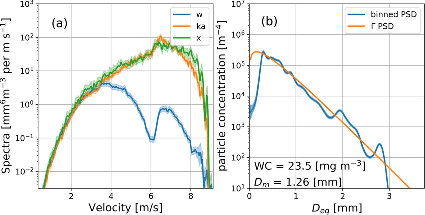
514                                                                                                  K. Mróz et al.: Spectra closure study

Table 1. Technical specifications and settings of the three vertically pointing radars operated during TRIPEx-pol at JOYCE-CF. Note that the
W-band radar is a FMCW system for which chirp repetition frequency, number of spectral average, Nyquist velocity and range resolution
change for different range intervals (see details in Dias Neto et al., 2019); values are provided here are for the lowest range gate region from
220 to 1480 m. Additionally, the radome of the W-band is equipped with a strong blower system which presents rain from accumulating.

                                 Specifications                               X-band     Ka-band       W-band
                                 Frequency (GHz)                                  9.4         35.5        94.0
                                 Pulse repetition frequency (kHz)                  10          5.0         6.6
                                 Number of spectral bins                         4048          512         512
                                 Number of spectral average                        10           20          13
                                 3 dB beam width (◦ )                             1.0          0.6          0.5
                                 Sensitivity at 1 km (dBZ), 2 s integration      −50          −70         −58
                                 Nyquist velocity (± m s−1 )                       80         10.5        10.2
                                 Range resolution (m)                              30           36          36
                                 Temporal sampling (s)                              2            2            3
                                 Lowest clutter-free range (m)                    300          400         300
                                 Radome                                            No           No         Yes

Figure 1. Time–height plots of radar variables measured at JOYCE on 24 November 2018: (a) X-band radar reflectivity factor (dBZ);
(b) dual-frequency ratio (DFR) of X- and Ka-bands (Z X − Z Ka ); (c) mean Doppler velocity (MDV, Ka-band); (d) lidar backscattering cross
section (note the difference in the range of the presented altitudes). The dashed lines indicate the top and the bottom of the melting level
derived from the Ka-band linear depolarization ratio (LDR). Black contour lines show isotherms derived from ECMWF analysis.

  Figure 1d shows the measured lidar backscattering cross                 the light signal (Delanoë and Hogan, 2010; Van Tricht et al.,
section from the ceilometer that is located less than 5 m                 2014). The presented measurements exclude their presence
away from the radars. Thanks to these measurements, periods               before 08:00 UTC for altitudes below 2 km. Afterwards, liq-
where the environmental conditions are favorable for riming               uid clouds are detected in the vicinity or within the melting
can by identified. Liquid clouds, which are essential for rim-            region. Unfortunately, due to strong attenuation no informa-
ing, appear as optically thick layers that strongly attenuate

Atmos. Meas. Tech., 14, 511–529, 2021                                                          https://doi.org/10.5194/amt-14-511-2021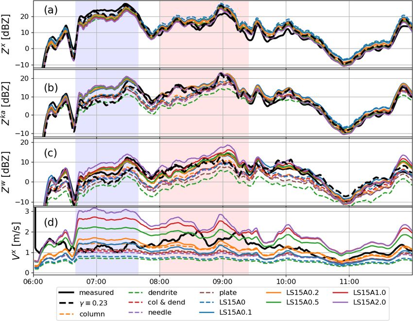
K. Mróz et al.: Spectra closure study                                                                                         515

tion about the presence of mixed-phase clouds aloft is avail-     theorem (Rodgers, 2000): it minimizes the cost function that
able.                                                             is composed of two equally weighted components. The first
                                                                  component computes the weighted distance to the triple-
                                                                  frequency spectra measurements, with the inverse variance of
3     Methodology                                                 the measurement error used as a weight. The other term cal-
                                                                  culates the deviation from the prior knowledge of the DSD.
This study aims at relating rain and ice microphysics imme-       For this retrieval, a widely adopted gamma-shaped DSD that
diately below and above the melting layer in stratiform pre-      fits the spectral measurements the best is used as the a pri-
cipitation. The overall logic of our approach is summarized       ori estimate (for more detail see Tridon and Battaglia, 2015).
in the schematic of Fig. 2. In a first approximation, retrieved   The backscattering cross sections of raindrops are computed
rain properties can be exploited to infer information about       with a T-matrix method using the Python code of Leinonen
the ice particles aloft via the MOSS assumption (follow black     (2014). The refractive index of water is computed at 10 ◦ C
arrows). Rainfall properties can be derived with less uncer-      using a model of Turner et al. (2016). Terminal velocities of
tainty than for ice because terminal velocities and backscat-     raindrops are interpolated from a dataset of Gunn and Kinzer
tering cross sections of raindrops are much more constrained      (1949) whereas the aspect ratio is calculated with a formula
than those of ice and snow particles. The predicted ice PSDs      of Brandes et al. (2005). The orientation of raindrops is as-
can then be used to simulate radar snow spectra but only once     sumed to follow a normal distribution of about 0◦ with a stan-
a “snow model” is selected; the comparison between simu-          dard deviation of 8◦ (Huang et al., 2008). Doppler spectra are
lated and measured snow spectra allows the establishment of       simulated according to the methodology described in Tridon
which snow models are more compatible with measurements           and Battaglia (2015) accounting for turbulence, vertical wind
and how realistic the MOSS assumption is. This bottom-up          and radar noise level.
approach is not novel and has already been applied in the past       The algorithm retrieves binned DSD along with two dy-
(e.g. Drummond et al., 1996; Battaglia et al., 2003).             namical parameters: turbulence and vertical wind.
   Here, thanks to the multi-frequency Doppler spectra ap-           An example of the measurements and the corresponding
proach, we can attempt a more elaborate “closure study”           retrieval is presented in Fig. 3. As expected, the spectral
where more accurate ice microphysical properties (and ver-        power for velocities below 4 m s−1 is nearly identical for the
tical wind) can be retrieved by matching spectra in ice at all    different frequencies, which is a result of Rayleigh (∝ D 6 )
frequencies via an optimal-estimation (OE) technique. For         scattering at all bands for drops smaller than approximately
the a priori ice PSD, we use the exponential PSD that best        1 mm. This Rayleigh part of the spectrum can be used to de-
fits the spectral measurements. From ice PSDs and vertical        termine differential path-integrated attenuation for different
wind, fluxes and PSD moments can be derived that can be           radar bands (Tridon et al., 2013). The spectrally derived dif-
directly compared to their counterparts in rain in a top-down     ferential attenuation has been accounted for, prior to the re-
approach, thus addressing the science questions (Sect. 1).        trieval. A significant reduction in the measured power at the
Such a procedure is featured in Fig. 2 with red-colored boxes     W-band compared to the other frequency measurements can
and arrows. We now describe in detail the key steps of the        be found for velocities exceeding 4 m s−1 . This fall velocity
whole approach.                                                   regime corresponds to particle sizes for which non-Rayleigh
                                                                  scattering effects increase and culminate at the first reso-
3.1    Rain DSD retrieval from multi-frequency radar              nant minimum, expected at 5.95 m s−1 according to Gunn
       Doppler spectra                                            and Kinzer (1949) data. The difference between the mea-
                                                                  sured and the anticipated position of the peak in the spectrum
Vertically pointing Doppler radars usually provide the full       corresponds to the vertical air velocity (Kollias et al., 2002).
Doppler spectrum, i.e., the spectral distribution of the re-         The blue line in Fig. 3b shows the retrieved DSD that
turn power over the range of the line-of-sight velocities. Be-    minimizes the cost function. This solution fits the measured
cause the raindrop terminal velocity is an increasing and         radar reflectivity with an accuracy of 0.25 dB at all frequency
well-constrained function of the raindrop size (Atlas et al.,     bands (not shown). As it can be seen, the widely used gamma
1973), these measurements can be used to resolve the drop         model (orange line) represents the bulk shape of the binned
size distribution (DSD), once the vertical wind and turbu-        DSD for drops up to 3 mm in size well. Nevertheless, some
lence are known (e.g., Williams et al., 2016; Tridon et al.,      subtle features of the Doppler spectra, such as an increase in
2017a; Giangrande et al., 2012).                                  the X- and Ka-band spectra around 6 m s−1 that corresponds
   Our DSD retrieval in the range bins below the melt-            to a local DSD maximum around 2 mm, cannot be modeled
ing zone closely follows the steps described in Tridon and        with the gamma function. It should be noted that although
Battaglia (2015). The only modification introduced here is        we assume a gamma-shaped PSD as a prior, no explicit func-
the extension of the observation vector from two to three fre-    tional shape is assumed for the retrieved DSD. This is an im-
quency bands in order to fully exploit the measurement ca-        portant advantage of the spectral retrieval as it allows the re-
pabilities of the radar site. The retrieval is based on Bayes’    trieval of complex DSDs, such as multi-modal distributions.

https://doi.org/10.5194/amt-14-511-2021                                               Atmos. Meas. Tech., 14, 511–529, 2021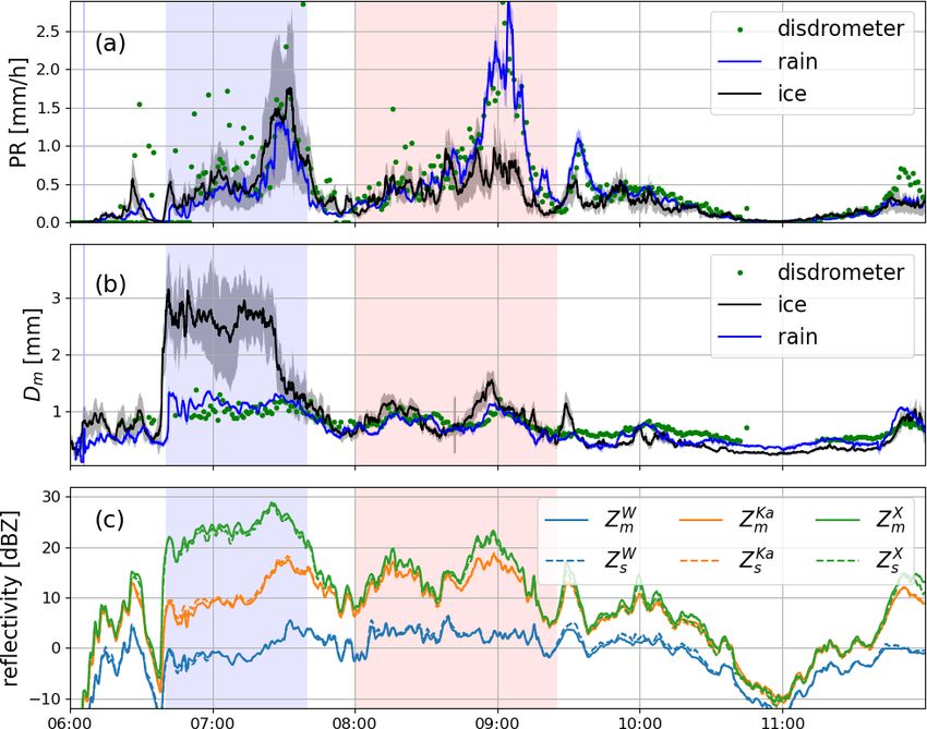
516                                                                                               K. Mróz et al.: Spectra closure study

Figure 2. Schematic illustrating the rationale of the spectra closure study: by linking microphysical properties of rain just below the melting
layer and of ice just above, the MOSS (black arrows) and the mass flux continuity (red arrows) assumptions can be evaluated.

                                                                          out. Due to the saturation problem of the GRAW humid-
                                                                          ity sensor the RH measurements are likely to be underes-
                                                                          timated, which is confirmed by lidar measurements where
                                                                          signatures of liquid clouds are present within the melting
                                                                          zone after 08:15 UTC (Fig. 1d), which indicates water va-
                                                                          por supersaturation conditions. Despite the potential incon-
                                                                          sistencies of our assumptions with the actual state of the at-
                                                                          mosphere, neglecting condensation and evaporation is used
                                                                          as a simplifying hypothesis that implies the flux of mass
                                                                          through the melting zone is conserved. Furthermore, follow-
                                                                          ing Szyrmer and Zawadzki (1999), Zawadzki et al. (2005),
Figure 3. (a) Doppler spectra measured in rain just below the melt-       and Matrosov (2008), no breakup and no interaction between
ing zone at 07:01:34 UTC. The green, orange and blue lines cor-           melting particles are assumed. Consequently, we might as-
respond to X-, Ka- and W-band data, respectively. The shaded ar-          sume that one ice particle is converted into one raindrop and
eas represent the measurement uncertainties. (b) The correspond-          the mass of each particle is preserved through the melting
ing binned DSD retrieval (blue) and the best fit gamma DSD (or-           layer (ms (Ds ) = mr (Dr )); thus the particle number flux is
ange). The x axis is the melted-equivalent diameter. The water con-       conserved at any size. Mathematically,
tent (WC) and mass-weighted mean diameter (Dm ) corresponding
to the binned DSD are shown as text in the corner.                        Ns (Ds ) [Vs (Ds ) + ws ] dDs = Nr (Dr ) [Vr (Dr ) + wr ] dDr , (1)

                                                                          where Ns and Nr denote the concentrations, and Vs and Vr
3.2   Deriving snow PSD from rain DSD via the                             are the still-air terminal velocities of snowflakes above the
      melting-only steady-state assumption                                freezing level (subscript s) and raindrops below the melting
                                                                          zone (subscript r), respectively. Vertical air motions ws and
In order to connect properties of ice with the properties of              wr in snow and rain are assumed to be negative when up-
rain, several assumptions are made. Firstly, processes across             wards. Vertical air motions in stratiform precipitation can be
the melting layer are assumed to be in steady state. Secondly,            assumed to be small compared to sedimentation velocities
effects of condensation or evaporation are neglected. The ra-             and hence they are neglected in the following. We will refer
diosonde launched at 09:00 UTC showed RH values exceed-                   to this set of assumptions as the “melting-only steady-state”
ing 90 % in the proximity to the freezing level, which ef-                hypothesis. It is convenient to formulate Eq. (1) in terms of
fectively excludes the possibility of evaporation. However,               the equivalent melted diameter Deq , which is a quantity pre-
the possibility of condensation on melting ice particles and              served through the melting process:
collision–coalescence with cloud droplets cannot be ruled

Atmos. Meas. Tech., 14, 511–529, 2021                                                         https://doi.org/10.5194/amt-14-511-2021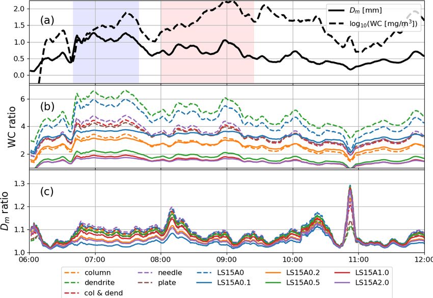
K. Mróz et al.: Spectra closure study                                                                                          517

                                                                   section as
                                                                                        λ4

Ns Deq Vs Deq dDeq = Nr Deq Vr Deq dDeq                                                                   dDeq
                                                                   Sλ,target (V ) =    5   2
                                                                                             N Deq σλ Deq        ,             (5)
                       Vr Deq
                                                                                     π |K|                  dV
⇒      Ns Deq = Nr Deq          .                          (2)
                         Vs Deq                                    where σλ gives the backscattering cross section of a target of
                                                                   a given size and |K|2 denotes its radar dielectric factor, and
Equation (2) expresses a link between the PSD of ice and the       V is its terminal velocity that is assumed to be dependent on
DSD of rain resulting from melting of snow. It shows how           the particle size. In this study a wide gamut of “snow models”
the V − D relationship for ice particles influences the shape      are considered to account for the large variability of scatter-
of the underlying distribution of rain. This relation should       ing and aerodynamical properties of ice crystals. Each snow
be understood as a first-order approximation that can be ap-       model entails a mass–size and an area–size relationship and
plied only when (1) the process is steady state, (2) collision,    provides size-dependent backscattering and extinction cross
coalescence and breakup are negligible, and (3) the relative       sections and fall speeds.
humidity is close to the saturation level.                            Broadly speaking two snow classes are analyzed in this
   To verify whether or where the MOSS assumption holds,           study. The first class consists of unrimed aggregates of dif-
the procedure shown in Fig. 2 as the black arrows is ap-           ferent ice habits, i.e., needles, plates, columns and dendrites.
plied. First, the triple-frequency measurements are extracted      These aggregates were created using the aggregation code
from the ranges just below the melting zone. Then, the             described in detail in Leinonen and Moisseev (2015). In to-
full Doppler spectra are used to retrieve a binned rain PSD        tal, approximately 30 500 aggregates were generated. The to-
(step A). By applying the MOSS assumption through the              tal number of monomers, as well as their size distribution
melting zone, the rain DSD is mapped into the PSD of ice           have been varied, in order to produce a large variety of shapes
(step B, Eq. (2)). The procedure is applied to 18 different        and densities. The monomers are distributed according to an
snow models, described in detail hereafter in Sect. 3.3. For       inverse exponential size distribution, with the characteristic
ease of display, only two models (needles and graupel) rep-        size ranging from 0.2 to 1 mm with a minimum and maxi-
resentative of two extremes are illustrated in the insets of       mum monomer size of 0.1 and 3 mm, respectively. The final
Fig. 2. The number concentration predicted for the ice parti-      aggregates consist of up to 1000 monomers and reach sizes of
cles just above the melting layer depends on the snow model        2 cm. The scattering properties were obtained with the self-
due to differences between their aerodynamical properties;         similar Rayleigh–Gans approximation (SSRGA; Hogan and
e.g. the aggregate models are characterized by higher parti-       Westbrook, 2014; Hogan et al., 2017). The SSRGA allows
cle concentration than rimed particles (compare the dashed–        the approximation of the scattering properties of an ensem-
dotted with the dashed line in Fig. 2, panel “PSD of ice”).        ble of self-similar, low-density particles (such as aggregates)
Doppler spectra corresponding to each snow model are de-           with an analytical expression and a set of corresponding fit-
rived with scattering and aerodynamical models (step C). The       ting parameters which characterize the structural properties
resulting simulated spectra at the three bands are compared        of the simulated snowflakes. For more detail on the SSRGA
with the actual measurements (step D). As a first closure at-      model used in this study see Ori et al. (2020a).
tempt, simulated radar reflectivities for ice (corrected for at-      The second considered class contains snow particles gen-
tenuation using the methodology described in Sect. 2.1) and        erated by Leinonen and Szyrmer (2015) and Leinonen et al.
Doppler velocities are compared with the measurements.             (2017) comprised of aggregates of dendrites with different
                                                                   degrees of riming. Three riming scenarios are included in
3.3   Snow models and Doppler spectrum simulator
                                                                   this dataset: particles, which grew by riming only (model C,
The Doppler spectrum measured by a vertically pointing             LS15C), aggregation and riming occurring simultaneously
radar transmitting at the wavelength λ is given by                 (model A, LS15A), or aggregation and riming occurring sub-
                                                                  sequently (model B, LS15B). The degree of riming is ex-
Sλ (V ) = Aλ × Sλ,w,target ∗Tair (V ),             (3)             pressed in terms of the equivalent liquid water path ranging
                                                                   from 0 kg m−2 for dry aggregates to 2 kg m−2 for graupel-
where Aλ is the two-way attenuation, Sλ,w,target is the reflec-    like particles. For instance, “LS15A1.0” denotes the model
tivity spectrum due to scattering from radar targets affected      of aggregates grown by simultaneous riming and aggrega-
by the vertical wind w, Tair is the air broadening kernel and ∗    tion, where particles passed through a layer of 1 kg m−2 of
denotes the convolution operator (for more detail see Doviak       cloud droplets.
and Zrnic, 1993). Note that the vertical wind only shifts the         The terminal velocities of individual particles in the two
spectrum, i.e.,                                                    snow classes are simulated for a standard atmosphere us-
Sλ,w,target (V ) = Sλ,target (V − w).                       (4)    ing the methodology of Böhm (1992). Then the expected
                                                                   velocity–size formula for each snow model is generated by a
The reflectivity spectrum, Sλ,target , can be expressed in terms   least-square difference fit of the generated data to the Atlas-
of the particle size distribution and the backscattering cross     like formula (Atlas et al., 1973) (suggested by Seifert et al.,

https://doi.org/10.5194/amt-14-511-2021                                                   Atmos. Meas. Tech., 14, 511–529, 2021
518 K. Mróz et al.: Spectra closure study
Table 2. Coefficients of the Atlas-like velocity–size relation (Eq. 6) the vertical velocity (step E). The uncertainties of these esti-
for different snow models. mates are set to 175 % for the turbulence and 0.16 m s−1 for
the vertical wind. These uncertainty values are derived from
Snow model α β γ the corresponding root-mean-square differences between the
(m s−1 ) (m s−1 ) (m−1 ) first guesses and the final estimates in rain over the analysis
Plate 1.41 1.43 1330.30 period. The retrieval is performed for all the selected models
Dendrite 0.89 0.90 1475.10 independently; the distance between the simulated and the
Column 1.58 1.60 1552.29 measured spectra, δmodel , is used as a measure of quality of
Needle 1.08 1.09 1781.26 the retrievals at each time step. The final estimate of the pos-
Col. & dend. 0.93 0.92 3628.93 terior PSD is derived as a weighted mean of all the solutions.
LS15A0.0 0.88 0.88 1626.17 The weights of each model, Wmodel , are computed as the soft-
LS15A0.1 2.16 2.16 660.76 max function of the distances to the spectral measurements,
LS15A0.2 2.09 2.09 936.83 i.e.,
LS15A0.5 2.43 2.43 1400.49 !−1
LS15A1.0 3.06 3.06 1199.37 2 X 2
−δmodel −δmodel
LS15A2.0 3.96 3.96 860.00 Wmodel = e e . (7)
LS15B0.1 1.25 1.25 1874.71 models
LS15B0.2 1.53 1.53 2144.21
LS15B0.5 2.29 2.29 1707.05 The snow retrievals that do not fit the measurements well do
LS15B1.0 3.25 3.25 1161.20 not contribute much to the final estimate due to the exponen-
LS15B2.0 4.59 4.59 715.88 tial decay, and the models that resemble the spectral measure-
LS15C 6.03 6.03 443.07 ments well contribute the most. The uncertainty estimate of
the final retrieval is derived from the weighted standard devi-
ation of the solutions. Uncertainties of individual retrievals
2014, as also applicable): are neglected in the final estimate because they are much
smaller than the variability corresponding to different snow
V Deq = α − β exp −γ Deq , (6) models. For the final solution, parameters like mass flux and
where α, β and γ are the optimal fitting parameters. The equivalent mass-weighted size can be computed and directly
shape of this fitting function is more realistic than the fre- compared with the same parameters in the rain (step F). This
quently used power-law fits since it can reproduce velocity allows us to achieve the “closure” and, for instance, to assess
saturation at larger sizes. Moreover, this parametrization is the validity of the flux continuity assumption.
characterized by considerably smaller root-mean-square er-
ror of the fit than the traditional power-law approach. A com-
4 Results
plete list of the fitting parameters corresponding to the differ-
ent snow models is given in Table 2. 4.1 DSD retrieval
3.4 Optimal estimation retrieval of ice PSD based on The goal of this study is to link the properties of rain with the
multi-frequency Doppler spectra characteristics of the overlying ice in stratiform precipitation.
As the rain DSD is the basis for this closure analysis, we first
While the bottom-up approach (comparing measured and
compare the spectra-retrieved DSD with the Parsivel2 mea-
simulated ice Doppler spectra based on rain DSD) only pro-
surements at the ground (Fig. 4). Despite the vertical dis-
vides a qualitative evaluation of the MOSS assumption, we
tance of approximately 700–800 m between the disdrometer
aim to directly derive the ice PSD from the measured multi-
and the radar-retrieved DSD just below the melting zone, the
frequency Doppler spectra just above the freezing level. The
two methodologies provide comparable results. The compar-
principal of this OE retrieval is very similar to the OE re-
ison reveals several advantages of the radar-derived DSDs.
trieval used for rain. Of course, the more complex scattering
First, it is able to retrieve smaller drop sizes (Deq < 0.5 mm)
and terminal velocity behavior of snow must be accounted
that are not detected by the disdrometer (Thurai et al., 2019;
for and will also likely increase the retrieval uncertainties.
Thurai and Bringi, 2018; Raupach and Berne, 2015). Sec-
In rain, we used the gamma model DSD that best fits the
ond, it has much higher temporal resolution (6 versus 60 s).
spectra (Tridon and Battaglia, 2015); in ice, the exponential
Third, it provides more reliable estimate of the number of
PSD that best fits the spectral ratios and the radar reflectivity
large drops that are very infrequent and may not be captured
at the X-band is used as a prior estimate. An uncertainty of
by the limited sampling volume of the disdrometer. Note that
a factor of 2 is assumed for the prior binned PSD concen-
the spectral method also has its limitations; e.g. the retrieval
tration. A prior for turbulence is derived using the method
for Deq < 0.2 mm must be interpreted with caution due to
proposed by Borque et al. (2016). The velocity of the slow-
increasing uncertainties (see Tridon et al., 2017a).
est detectable radar targets in ice is used as the prior for
Atmos. Meas. Tech., 14, 511–529, 2021 https://doi.org/10.5194/amt-14-511-2021K. Mróz et al.: Spectra closure study 519
coherent peak, but only up to 1.75 km in altitude. The spec-
tra from the riming period (Fig. 5b) are characterized by a
much thicker melting layer (approximately 400 m) and by
bimodal distributions both in rain and in ice. The secondary
ice mode appears approximately 1–1.5 km above the melting
level, which corresponds to temperatures ranging between
−4 and −6.5 ◦ C according to the radiosonde launched at
09:00 UTC. There is high vertical variability in the position
of the main peak, which indicates more dynamical condi-
tions. The secondary mode increases its intensity while ap-
proaching the melting level but remains clearly separated
Figure 4. (a) DSD measurements at the ground with a Parsivel dis- from the main peak (see Fig. 5b). In the melting zone this
drometer. (b) DSD retrieved with multi-frequency Doppler spec- separation disappears, and the fall speed of the secondary
tra below the melting zone at ca. 700–800 m. The period shaded in mode increases so that the secondary peak stretches out in
blue corresponds to the region of large DFRX-Ka values above the the velocity domain and merges with the primary mode. This
melting layer that indicates aggregation. The period of enhanced behavior excludes the scenario of super-cooled drizzle above
Doppler velocities indicating riming is marked in red. the freezing level as it was discussed before. The LDR mea-
surements at the Ka-band (Fig. 5d) are in agreement with this
theory. The slowly falling mode corresponds to LDR reach-
Throughout the rest of the paper, the period of large ing −15 dB; such values are much larger than those expected
DFRX-Ka values (aggregation) is marked by the light blue for nearly spherical drizzle droplets. This spectral feature is
color, whereas the domain of enhanced Doppler velocity similar to the enhanced LDR signatures found in Oue et al.
(riming) is shaded in red. The DSDs during the two peri- (2015b) and Giangrande et al. (2016). They related the high-
ods are quite distinct: the aggregation-dominated period (al- LDR region to columnar ice crystals grown in liquid-cloud
most 1 h) is associated with a larger number of big drops and layers through secondary ice production. Interestingly, the
almost exponential DSDs. During the following riming pe- high-LDR signature of the small ice mode can also be de-
riod, a much larger concentration of small droplets and multi- tected during the melting of these particles, which might im-
modalities of the DSD are found. There are two potential ply that the columnar crystals are of considerable size as they
sources of this high concentration of small droplets: super- seem to maintain their asymmetric shape for quite some time
cooled drizzle that forms aloft by coalescence of supercooled until they are completely melted into drops (Fig. 5d). During
cloud droplets or secondary ice crystals, e.g. generated by aggregation, the opposite is true, i.e., the Ka-band LDR of
the Hallett–Mossop process (Mossop, 1976). In the first sce- large snowflakes is clearly larger than that of small ice crys-
nario, the slowly falling mode does not significantly change tals. This increase in LDR for large aggregates is principally
its intensity and position in the Doppler spectrum while pass- consistent with scattering simulations of realistic snowflakes
ing through the melting zone (Zawadzki et al., 2001) be- in Tyynelä et al. (2011, their Fig. 7) where LDR values are
cause there is no phase change of the particles. In the sec- predicted to increase for maximum sizes exceeding 5 mm.
ond scenario, the melting process changes the velocities and Note that the secondary mode in rain (Fig. 5b) appears
backscattering properties of the hydrometeors, thus resulting to be disconnected from the secondary mode in ice during
in a shift and a change in amplitude of the spectral power riming. At an altitude of approximately 800 m there is a
of the mode. The following analysis of the evolution of the clear gap between them, which is shown by the black box
Doppler spectra from the ice to the rain part is therefore ex- in Fig. 5b. This separation is present over several minutes,
pected to better explain the source of the small droplet mode. which suggests that the small rain droplets do not originate
from the melting of ice crystals; thus the assumption of one-
4.2 Doppler spectral features during the investigated to-one correspondence between ice particles and raindrops
time periods may not hold for this profile. Lidar measurements (Fig. 1d)
indicate the presence of a small droplets within the melting
Differences between riming and aggregation regimes are re- zone; therefore the secondary mode in rain is likely to be
flected in the Doppler spectra that are shown in Fig. 5. Dur- drizzle generated by this liquid layer or melting ice crystals
ing aggregation, the spectra in the ice phase are unimodal (too little to be detected by the radar) that underwent rapid
and the position of the peak is relatively constant at different growth through collision–coalescence processes while pass-
heights, which indicates weak vertical air motion (Fig. 5a). ing through the cloud.
The transition from ice to rain, corresponding to a strong
broadening of the spectra, happens very rapidly within less
than 200 m. The “aggregates” have a consistent spectral peak
to 4 km, while the “rimed” particles also show a vertically
https://doi.org/10.5194/amt-14-511-2021 Atmos. Meas. Tech., 14, 511–529, 2021520 K. Mróz et al.: Spectra closure study
creased compared to the small ones. This causes a reduction
of the mean mass-weighted diameter (Dm ) during melting;
i.e., the expected characteristic size of the DSD below the
melting zone is up to 30 % smaller than the corresponding
size in the ice aloft (Fig. 6c), and this change is purely as-
cribed to aerodynamic effects combined with the mass flux
conservation constraint. Note that for the majority of the par-
ticle models, the associated difference in Dm usually does
not exceed 10 %; for rimed particles this change is even less
pronounced and the characteristic melted-equivalent size is
practically preserved.
4.3.1 Discussion of the validity of the melting-only
steady-state assumption
According to the “reflectivity flux” method proposed by
Drummond et al. (1996) and Zawadzki et al. (2005), the ratio
of the reflectivity fluxes in snow and rain,
Zs VD,s
γ≡ , (8)
Zr VD,r
is equal to µ ≡ (ρw /ρi )2 |Ki |2 /|Kw |2 = 0.23, where the
Figure 5. W-band Doppler spectra (a, b) and Ka-band spectral
LDR (c, d). Panels (a) and (c) correspond to the measurements at mean Doppler velocity is denoted by VD , and the subscripts
07:01 UTC dominated by aggregation; panels (b) and (d) were sam- s and r indicate sampling in snow and rain, respectively,
pled at 08:58 UTC, when mean Doppler velocities indicate the pres- whereas the subscript i indicates ice. The relation is only
ence of rimed particles. Only the data where SNR> 3 dB are shown. valid for Rayleigh targets (which should hold for our X-band
The black box in panel (b) marks the secondary modes in ice and data) and under the MOSS assumption. Although the factor
rain. Positive Doppler velocities indicate motions towards the radar. µ was computed assuming constant ice density, the deriva-
tion is based on the formula of Debye (|Ks |/ρs = const),
which implies the reflectivity of ice particles depends only
4.3 Inferring ice PSD based on rain DSD via the on their mass not density. Therefore, the value of µ is in-
melting-only steady-state assumption dependent of the snow morphology. Values between 0.15
and 0.30 are still compatible with the MOSS assumption
In a first step, we derive the DSD of ice from the PSD of when plausible vertical air motions (i.e., wr = ±1 m s−1 and
rain via the MOSS assumption (Eq. 2). Figure 6a shows ws = ±0.5 m s−1 ) are allowed (Drummond et al., 1996). If
the DSD mass-weighted mean diameter (Dm ) and the wa- we introduce a normalized parameter in logarithmic units,
ter content (WC), as it is retrieved from the Doppler spec- γ
tra in the rain below the melting region. The aggregation γn [dB] = 10log10 , (9)
0.23
period is characterized by smaller water content but larger
characteristic size of raindrops compared to the riming pe- values of γn higher (lower) than 0 dB are indicative of
riod. With the MOSS assumption, the ice WC and the melted breakup (collision–coalescence) or of a nonstationary pro-
Dm of snow depend on the V − D relationship of ice and on cess. Note that this method is based purely on the radar mea-
the rain DSD. Because the velocities of raindrops are larger surements. Thus it is not dependent on any snow or rain
than those of the same-mass snowflakes of any density, it model. The methodology has been recently applied to X-
follows that Ns (Deq ) > Nr (Deq ). Consequently, the assump- band profiler data by Gatlin et al. (2018), where it was found
tions made in Sect. 3.2 imply that the ice WCs at the freez- that thicker melting layers generally correspond to negative
ing level are always larger than the rain WCs just below the γn , i.e., are indicative of dominant coalescence and/or aggre-
melting zone (Fig. 6b). In the most extreme scenario, i.e., gation while transitioning from ice to liquid. Moreover, by
in the case of slow dendrite aggregates, ice WC can be 7 combining Eq. (8) for γ ≡ 0.23 with Eq. (9), the ice reflec-
times larger than rain WC. For rimed snowflakes, this differ- tivity that would correspond to the MOSS assumption can be
ence is much smaller, but still a factor of 2 is expected for derived:
graupel-like particles. Because the ratio Vr (Deq )/Vs (Deq ) is Zγn ≡0 = Zm − γn , (10)
not constant but rather monotonically increases with size, the
ice PSD is not simply a scaled version of the underlying DSD where Zm is the reflectivity measured above the freezing
of rain; i.e., the number concentration of large particles is in- level.
Atmos. Meas. Tech., 14, 511–529, 2021 https://doi.org/10.5194/amt-14-511-2021K. Mróz et al.: Spectra closure study 521
Figure 6. (a) Derived Dm and WC (in log units) for the rain DSD just below the melting zone. (b) Relative change of the WC when passing
ice /D rain . Different colors correspond to different ice
from rain to ice, i.e., WCice / WCrain . (c) The same as panel (b) but for Dm , i.e., Dm m
models as indicated in the legend. Dashed lines correspond to unrimed aggregates, and solid lines denote rimed particles. Blue and red
shading indicates aggregation- and riming-dominated periods, respectively.
Figure 7. The normalized ratio between the reflectivity fluxes in ice and rain in the vicinity of the melting level as defined by Eq. (9).The
grey shading highlights the uncertainty introduced by the variability in the vertical wind.
In order to match the data below and above the melting lates between −6 and 4 dB. This non-uniform behavior can
layer more precisely, for each 15 min time window the op- be, at least partially, caused by a more turbulent environment,
timal time lag that maximizes the correlation between the which might favor more non-stationary conditions. Also, the
X-band reflectivity in ice and rain is derived. All the results presence of fall streaks (e.g., around 09:00 UTC) can be
that follow use this optimal matching in time. Most of the seen as an indication for more heterogeneous conditions.
time, γn is within the uncertainty limits introduced by ver- Moreover, riming particles have a broader range of terminal
tical air motion (see Fig. 7). The root-mean-square differ- fall velocities (compared to aggregates of the same mass),
ence over the case study between the ice reflectivity predicted which favors collision–coalescence processes and thus vio-
with the MOSS hypothesis and the measurements is equal to lates the underlying MOSS assumption. Within the uncer-
2.7 dB. The most consistent deviation from the uncertainty tainty introduced by the assumed vertical wind variability,
limits is reported during the period when large snow aggre- our analysis confirms that the period before 08:00 UTC is
gates are expected above the 0 ◦ C level. Large positive γn mainly characterized by breakup whereas the period after
values consistently suggest breakup as the main process oc- 08:00 UTC is dominated by collision–coalescence within the
curring within the melting zone (Fig. 7). The behavior of γn bright band. This corroborates the previous hypothesis of
is more variable during the period of riming, where it oscil-
https://doi.org/10.5194/amt-14-511-2021 Atmos. Meas. Tech., 14, 511–529, 2021522 K. Mróz et al.: Spectra closure study
preponderance of aggregation before 08:00 UTC and of rim- The ranges of simulated Ka- and W-band reflectivities is
ing after 08:00 UTC within the snow layer. much wider than that at the X-band, with differences be-
One of the difficulties of interpreting profile-type measure- tween heavily rimed particles and unrimed aggregates reach-
ments is that they do not provide a full 3D picture of the at- ing 10 and 14 dB at the Ka- and W-band, respectively. This is
mosphere, but just a 2D slice. Therefore, the presented con- related to the fact that backscattering cross sections in non-
clusions are based on the assumption that the observed sys- Rayleigh scattering conditions become increasingly sensitive
tem is locally homogeneous, i.e., despite horizontal winds to the snow particle type and density rather than simply being
the measurements taken below the melting layer correspond proportional to the square of the mass. Because the variabil-
to the evolution of the ice PSD measured aloft. Considering ity of simulated Ka- and W-band reflectivities for different
the horizontal wind speed within the bright band (approx. models is much larger than the range of γn values, the triple-
1.8 m s−1 during the “aggregation” period according to the frequency reflectivity data are more informative about the
ECMWF model) and the time needed for the particles to melt particle models that are more suitable during specific time
(approx. 3 min based on the MDV data), the precipitating periods. For a qualitative comparison, γn is used as a cor-
system must be uniform over 325 m to meet this criterion. rection factor to the number concentration that makes triple-
Because the beam width of the X-band radar at the altitude frequency measurements consistent with the MOSS simula-
of the melting zone is only 15 m, it is possible that the higher tions. This is done by reducing the measured reflectivities
ice-phase reflectivity flux relative to rain can be a result of a by γn derived for the X-band (ZγXn ≡0 = Z X − γn ; ZγKa n ≡0
=
horizontal gradient of the reflectivity that, for example, corre- Z Ka − γn ; ZγWn ≡0 = Z W − γn ). The result of this correction is
sponds to the storm intensification along the wind direction. shown as the dashed black line in Fig. 8a–c. With this cor-
Note that, for most of the aggregation period the precipita- rection applied to the triple-frequency reflectivity data, it be-
tion rate increases over time (see Fig. 9a), which supports comes clear that for the period before (after) 07:45 UTC, only
this alternative interpretation. models of unrimed aggregates (rimed particles) plotted with
dashed (continuous) colored lines are consistent with the
4.3.2 Towards reconciling radar moments at the top of multi-frequency observations. Similar conclusions are drawn
the melting layer by selecting an adequate snow when considering the simulated and observed Doppler veloc-
model ities (Fig. 8d).
The γn adjustment applied to all frequencies is a very
Encouraged by the results on the matching of the reflectiv-
crude approximation but it provides a significant improve-
ity fluxes in rain and ice, in the following section we test
ment in terms of compatibility between triple-frequency-
whether the MOSS assumption combined with the informa-
measured Doppler spectra moments. However it implies an
tion on the DSD in rain can help in constraining microphys-
“extensive” adjustment of the snow PSD; for instance a
ical properties of ice in the vicinity of the melting level. For
±3 dB correction corresponds to doubling or halving the
this purpose, the reflectivities at the three different frequen-
mass flux through the melting layer. Changes in the shape of
cies are simulated for all the different snow models for the
the PSD could in principle lead to better fitting of the mea-
PSDs predicted with the MOSS assumption (Eq. 2). Regard-
surements and more continuous change in the mass flux. This
less of the ice morphology the X-band reflectivity simula-
is what is investigated next with the more exhaustive closure
tions cluster close together with a standard deviation between
study.
them ranging from 1 to 1.5 dB only (Fig. 8a). The envelope
of simulations follows the X-band reflectivity predicted by
4.4 Closure study: connecting PSD and mass flux
assuming γn = 0 dB (denoted later as ZγXn ≡0 ), which is plot-
retrieved above and below the melting layer
ted as a dashed black line in Fig. 8. The largest difference
in the simulated reflectivities occurs between the models of Instead of only a qualitative comparison of the MOSS as-
graupel (LS15C) and aggregates of dendrites; this discrep- sumption (step D in the schematic Fig. 2), we are now able to
ancy reflects differences in the ice water content for different directly analyze the differences in mass flux and PSD above
snow models (see Fig. 6b) but is always smaller than 5 dB. and below the melting layer by using the associated retrieval
The inter-model variability of the reflectivity simulations is results for rain and ice. In this way, we can quantify the dif-
comparable to the variability of the γn , which suggests that ferences according to the dominating processes, which is ex-
X-band radar data alone can provide very limited guidance pected to also be relevant for future modeling studies.
on the density of snow above the melting zone, even when The PSD multi-spectral retrieval described in Sect. 3.4
detailed information of the rain, which originated from it, (step E in Fig. 2) is applied to the whole period, and the re-
is available. The X-band simulations mirror the finding of sults are presented in Fig. 9. The mass flux and Dm above
Sect. 4.3.1, i.e., during the entire period of strong aggrega- the melting level (continuous lines in Figs. 9a–b) are derived
tion, the simulations underestimate the measurements by ap- as an ensemble mean of the multi-frequency spectral OE ice
proximately 5 dB, which is a signature of the MOSS assump- retrievals where each solution is weighted by its distance to
tion being invalid at that time period. the observed spectra as is shown in Fig. 10. The most prob-
Atmos. Meas. Tech., 14, 511–529, 2021 https://doi.org/10.5194/amt-14-511-2021You can also read


