MARSIS: Mars Advanced Radar for Subsurface and Ionosphere Sounding
←
→
Page content transcription
If your browser does not render page correctly, please read the page content below
MARSIS: Mars Advanced Radar for Subsurface
and Ionosphere Sounding

G. Picardi1, D. Biccari1, R. Seu1, J. Plaut2, W.T.K. Johnson2, R.L. Jordan2, A. Safaeinili2, D.A. Gurnett3,
R. Huff 3, R. Orosei4, O. Bombaci5, D. Calabrese5 & E. Zampolini5
1
    Infocom Department, ‘La Sapienza’ University of Rome, Via Eudossiana 18, I-00184 Rome, Italy
     Email: aclr@aerov.jussieu.fr
2
  Jet Propulsion Laboratory, 4800 Oak Grove Drive, Pasadena, CA 91109, USA
3
  Department of Physics and Astronomy, University of Iowa, Iowa City, IW 52242-1447, USA
4
  CNR/IAS, Planetology Department, Via del Fosso di Cavaliere, I-00133 Rome, Italy
5
  Alenia Spazio S.p.A., Via Saccomuro 24, I-00131 Rome, Italy

This paper describes the science background, design principles and the expected
performance of the Mars Advanced Radar for Subsurface and Ionosphere
Sounding (MARSIS), developed by a team of Italian and US researchers and
industrial partners to fly on the ESA Mars Express orbiter. The unique
capability of sounding the martian environment with coherent trains of long-
wavelength wide-band pulses, together with extensive onboard processing, will
allow the collection of a large amount of significant data about the subsurface,
surface and ionosphere. Analysis of these data will allow the detection and 3-D
mapping of subsurface structures down to several kilometres below the surface,
the estimation of large-scale topography, roughness and reflectivity of the
surface at wavelengths never used before, and the production of global and high-
resolution profiles of the ionospheric electron density (day and night). Finally,
the MARSIS frequency-agile design allow the sounding parameters to be tuned
in response to changes in solar illumination conditions, the latitude and other
factors, allowing global coverage to be achieved within the Mars Express
baseline orbit and mission duration.

The set of scientific objectives for MARSIS was defined in the context of the                1. Introduction
objectives of the Mars Express mission and within the more general frame of the open
issues in Mars studies. The primary objective is to map the distribution of liquid and
solid water in the upper portions of the crust of Mars (Carr, 1996). Detection of such
water reservoirs will address key issues in the hydrologic, geologic, climatic and
possible biologic evolution of Mars, including the current and past global inventory
of water, mechanisms of transport and storage of water, the role of liquid water and
ice in shaping the landscape of Mars, the stability of liquid water and ice at the surface
as an indication of climatic conditions, and the implications of the hydrologic history
for the evolution of possible martian ecosystems.
   Three secondary objectives are also defined for MARSIS: subsurface geologic
probing, surface characterisation and ionosphere sounding. The first is to probe the
subsurface of Mars, to characterise and map geologic units and structures in the third
dimension. The second is to acquire information about the surface: to characterise the
surface roughness at scales of tens of metres to kilometres, to measure the radar
reflection coefficient of the upper surface layer, and to generate a topographic map of
the surface at approximately 10 km lateral resolution. The final secondary objective
is to use MARSIS as an ionosphere sounder to characterise the interactions of the

                                                                                                               1
SP-1240

                             solar wind with the ionosphere and upper atmosphere of Mars. Radar studies of the
                             ionosphere will allow global measurements of the ionosphere electron density and
                             investigation of the influence of the Sun and the solar wind on the ionosphere.

    2. Composition Models    In this section, models of the composition of the upper layers of Mars are described,
       of the Upper Layers   based on the recent literature and classical Mars studies.
                                 The state and the distribution of H2O in the martian megaregolith are a function of
                             crustal thermal conductivity, geothermal heat flow, ground-ice melting temperature
                             and the mean temperature at the surface (this last is the only quantity varying
                             systematically with latitude). These factors determine the thickness of the cryosphere,
                             which is the layer where the temperature remains continuously below the freezing
                             point of H2O. Although the mean annual surface temperatures vary from about 220K
                             at the equator to about 155K at the poles, the annual and secular surface temperature
                             variations determine periodic freezing and melting of any H2O present down to a
                             depth of about 100 m. The cryosphere extends below this ‘active layer’ to the depth
                             where the heat flux from the interior of the planet raises the temperature above the
                             melting point of ground-water ice. Below the cryosphere, H2O in the pore space can
                             only be in liquid form.
                                 Estimates of the depth of the melting isotherm range from 0 km to 11.0 km at the
                             equator, and from 1.2 km to 24 km at the poles, according to different values of the
                             parameters found in the literature. Liquid water may persist only below such depths;
                             moreover, liquid water would diffuse towards the bottom of the regolith layer and
                             thus could lay further below, although local conditions may still offset the above
                             considerations. A nominal depth in the range 0-5000 m is assumed.
                                 Estimates of the desiccation of the martian megaregolith, via ice sublimation in the
                             cryosphere, yield values of the depth at which ice is still present ranging from zero to
                             several hundred metres. A nominal depth in the range 0-1000 m is assumed.
                                 The interfaces most likely to be detected by MARSIS, being closer to the surface,
                             are the contact between the desiccated regolith and the permafrost, and the interface
                             between a subterranean reservoir of liquid water and the cryosphere. These are the
                             basic scenarios for the detection and identification of water-related interfaces in the
                             martian subsurface.
                                 The structure of the martian crust is the result of many different processes, given the
                             complex geological history of the planet. However, it appears that the most significant
                             on a global scale are impact processes, which have played a major role in the structural
                             evolution of the crust by producing and dispersing large quantities of ejecta, and by
                             fracturing the surrounding and underlying basement. It is estimated that, over the course
                             of martian geologic history, the volume of ejecta produced by impacts was sufficient to
                             have created a global blanket of debris up to 2 km thick. It is likely that this ejecta layer
                             is discontinuously interbedded with volcanic flows, weathering products and
                             sedimentary deposits, all overlying a heavily fractured basement.
                                 A 50% surface porosity of the regolith is consistent with estimates of the bulk
                             porosity of martian soil as analysed by the Viking Landers. A value this high requires
                             that the regolith has undergone a significant degree of weathering. A lower bound for
                             the surface porosity can be taken at 20%, derived from the measured porosity of lunar
                             breccias. An equation of the decline of porosity with depth owing to the lithostatic
                             pressure can be obtained by adapting a similar equation devised for the Moon, based
                             on seismic data unavailable for Mars. The equation is of the form:
                                                                                      z

                                                                  £1z2  £102 e K                                     (1)

                                where Φ(z) is the porosity at depth z, and K is a decay constant that, for Mars, can
                             be computed by scaling the measured lunar decay constant for the ratio between the
                             lunar and martian surface gravitational acceleration, under the assumption of
                             comparable crust densities. The resulting value for Mars is K = 2.8 km.

2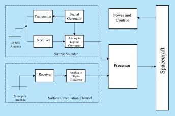
scientific instruments

Table 1. Dielectric properties of the subsurface material.

                        Crust Material                  Pore-Filling Material
               Andesite             Basalt         Water Ice          Liquid Water

εr                    3.5             7.1             3.15                 88
tan δ             0.005              0.014          0.00022              0.0001

Table 2. Value ranges of the surface geometric parameters.

               Large-Scale Model                         Small-Scale Model
        rms slope           correlation length     rms slope           rms height

        0.01-0.1 rad           200-3000 m          0.1-0.6 rad           0.1-1 m
        (0.57-5.7°)                                (5.7-34.3°)

   It appears almost certain from morphologic and chemical evidence, as well as from
SNC meteorites, that the martian surface is primarily basaltic. However, it could have
a thin veneer of younger volcanics overlying a primitive crust. Whether this primitive
crust is basaltic, anorthositic like the Moon, granodioritic like the Earth’s continents
or some other kind of composition, is unknown. The NASA Pathfinder APXS
analyses of rocks and soils confirm the basaltic nature of Mars’ surface. Chemical
classifications of lavas show that the Barnacle Bill and Yogi rocks are distinct from
basaltic martian meteorites. These rocks plot in or near the field of andesites, a type
of lava common at continental margins on Earth. Although a multitude of different
chemical compositions is present at the surface of Mars, it is necessary to select a few
representative materials as most meaningful for electromagnetic studies. Given the
above considerations about the nature of the martian crust, andesite and basalt were
chosen because their dielectric constants are end-members of the range within which
the martian surface materials may vary.
   The dielectric properties of the crust end-member materials, together with those of
the water and ice filling the pores, are listed in Table 1.
   To summarise, the reference models representing the two most likely detection
scenarios for a Mars orbital sounder at km depths are (Fig. 1):

Ice/water interface detection. According to the model, the porosity of the martian
   megaregolith is maximum at the surface and its decay with increasing depth is
   given by the exponential law in Eq. (1). The pores are filled with ice from the
   surface down to a depth below which liquid water is stable and becomes the pore-
   filling material. The change causes a discontinuity of the overall dielectric
   constant, which can be detected by the radar sounder. The ice/water interface is
   believed to be at a depth of between 0 m and 5000 m.
Dry/ice interface detection. This model is based on the same assumptions as the
   ice/water model with respect to the megaregolith properties. However, the pore-
   filling material here is considered to be gas or some other vacuum-equivalent
   material up to a certain depth below which ice fills the pores. Hence the interface
   to be detected is between dry regolith and ice-filled regolith, expected to be at a
   depth of between 0 m and 1000 m.

 These models will be used to estimate the penetration performance under typical
MARSIS operating conditions.

                                                                                                               3
SP-1240
Fig. 1. Martian crust stratification models.
Simple 2-layer structures are proposed. The
discontinuity is created by a change in the
pore-filling material. a: ice/water interface
detection; b: dry/ice interface detection.
3. Surface Characterisation Images of the surface from the Viking Landers and Mars Pathfinder depict a gently
undulating surface strewn with rocks ranging in size from a few centimetres to
metres. Although these images cover only a minute portion of the planet, Mars’
thermal and radar properties have prompted extensive modelling of a rock
population scattered over the entire surface. The surface geometric structure is thus
characterised in terms of a large-scale morphology on which a small-scale geometric
structure, of rocks, is superimposed. It is assumed that the surface can be described
as a random distribution of heights, characterised by a variance σh, a correlation
length L and a local surface rms slope ms. By assuming that the height distribution
is Gaussian, then ms = √2 σh / L, so that the distribution is completely determined
once the values of two of these parameters are known. The terms large-scale and
small-scale refer to different approximations in the modelling of the radar
backscattering coefficient; the divide between large-scale and small-scale is
essentially the radar wavelength.
Topographic data can be used to derive the large-scale geometry of the surface. The
global topographic maps of Mars currently available were compiled from several
types of measurements with different resolutions and sources of uncertainties. These
data do not provide a complete, global picture of Mars’ topography, but allow the
inference that elevation changes, although relevant in magnitude, do not involve
average slopes greater than 5° (0.1 rad), and often much less. Also, the correlation
lengths for the topography appear to be rather large, perhaps of the order of tens of
kilometres.
To characterise the surface geometry at scales smaller than the radar resolutions, it
is necessary to use proper data sets: measured values for Mars are in the range 0.7-
13°, averaging 2°, with a remarkable diversity from place to place over the surface.
Such values refer to scales that, according to model interpretations, range from a few
tens to a few hundred metres.
To summarise, plausible ranges for the parameters describing the surface geometry
are listed in Table 2.
Recent attempts to describe the structure of planetary surfaces by means of fractals
have also been taken into account. Tests on MGS/MOLA data have shown that the
Hurst exponent (H) with very high probability lies in the range 0.7-1 and the rms
slope (s(∆x)) extrapolated with a lag ∆x = 166 m is lower than 0.05.
4. Characterisation The study of the martian ionosphere is important not only as a topic in its own right,
of the Ionosphere but also because the ionosphere has a strong influence on the subsurface and surface
soundings. Electromagnetic radiation cannot propagate through an ionised gas at
frequencies below the electron plasma frequency, given by fp = 8980 √Ne Hz, where
4scientific instruments
Fig. 2. a (above): typical plasma frequency
vertical profile; b (left): plasma frequency
behaviour with solar zenith angle.
Ne is the electron number density in cm–3. A typical profile of the electron plasma
frequency in the dayside martian ionosphere is shown in Fig. 2a, based on plasma
density measurements from the Viking Landers (Hanson, 1977). Usually the electron
plasma frequency on the dayside of Mars has a single, well-defined maximum, at an
altitude of 125-150 km. Radio waves incident vertically on the ionosphere are
reflected at the point where the wave frequency is equal to the electron plasma
frequency. Transmission through the ionosphere is possible only at frequencies above
the maximum electron plasma frequency in the ionosphere, fp (max). Figure 2b shows
a plot of fp (max) versus solar zenith angle. The solid dots give the plasma frequency
obtained from radio occultation measurements (Zhang et al., 1990a; 1990b), and the
solid lines give extrapolations using the Chapman theory of planetary ionospheres.
Subsurface soundings are possible only at frequencies greater than fp (max). Since
they require frequencies as low as possible, the global distribution of the ionospheric
electron density (hence plasma frequency) becomes an important factor in selecting
the operating frequency of the sounder and the optimal orbital strategy for data
collection. The lowest frequency that can penetrate the martian ionosphere varies
from about 4 MHz on the dayside to somewhat below 1 MHz on the nightside.
Clearly, the best region for carrying out subsurface soundings is on the nightside, at
solar zenith angles greater than 90°. Unfortunately, very little is known about the
ionosphere on the nightside. A typical nightside maximum plasma frequency appears
to be about 800 kHz. From our knowledge of the ionosphere of Venus, for which
better nightside electron density measurements are available, it is likely that there are
isolated regions on the nightside of Mars where the plasma frequency extends well
below 800 kHz.
Even when the sounding frequency is above fp (max), the ionosphere still has an
effect on the radar signal. As is well known (Stix, 1964), the index of refraction for
an electromagnetic wave propagating through an unmagnetised plasma is given by
n = [1-(fp /f )2]1/2. Even at frequencies several times the plasma frequency, the index of
refraction has a noticeable deviation from the free-space value of n = 1. This
deviation causes a frequency-dependent time delay, called dispersion, that distorts the
shape of the radar pulse. It is easily demonstrated that the phase shift induced by the
ionosphere over the ∆f = 1 MHz bandwidth of the radar chirp signal is substantial,
approximately 200 rad for a centre frequency at f = 2 fp(max), and 5 rad at
5SP-1240
f = 10 fp(max). Since the sounder must almost certainly operate at frequencies below
10 fp(max), it follows that we must be prepared to remove the dispersive effects of the
ionosphere, otherwise the signal-to-noise ratio and range resolution of the radar signal
would be severely degraded in the chirp compression process.
5. MARSIS Orbital The baseline orbit for Mars Express has a periapsis distance of 250 km, apoapsis
Requirements distance of 10 142 km, inclination 86.35° and period of 6.75 h. Figure 3 shows the
tangential and radial components of the satellite’s orbital velocity as a function of
altitude above the equatorial radius. MARSIS is designed to perform subsurface
sounding during each orbit when the altitude is lower than about 800 km; for the
baseline orbit that means a period of about 26 min. This allows mapping of about
100° on the surface on each orbit, allowing extensive coverage at all latitudes within
the nominal mission duration. To achieve this global coverage, MARSIS is designed
to support both dayside and nightside operations, although performances are
maximised during the night (solar zenith angle > 80°), when the ionosphere plasma
frequency drops off significantly and the lower frequency bands, which have greater
penetration capability, can be used. Ionospheric soundings will be also carried out by
MARSIS on certain passes when the orbiter is at an altitude up to 1200 km, both
during day and night time.
6. Measurement Concept 6.1 Subsurface and surface sounding
and Experiment The sounder’s principle of operation is explained in Fig. 4. The electromagnetic wave
transmitted by the antenna impinges on the surface, producing a first reflection that
Description propagates back to the radar, generating a strong return signal received at time
t0 = 2H/c, H being the spacecraft height and c the speed of light in vacuum. However,
thanks to the long wavelengths employed, a significant fraction of the energy
impinging on the surface is transmitted into the crust and propagates down with a
decreased velocity v = c/n (n is the refractive index of ice related to the real dielectric
constant εr by n = √εr) and an attenuation proportional to the penetration depth (z), to
the wavelength (λ) and to the material loss tangent (tan δ, defined as the ratio of the
imaginary part to the real part of the complex dielectric constant, tan δ = εi/εr). Should
subsurface dielectric discontinuities be present at depth z0 below the surface, additional
reflections would occur and the echoes would propagate back through the first layer
medium and then to the radar, generating further echo signals, much weaker than the
front surface signal, with time delay t0 + 2z0 /v. As a consequence, time-domain
analysis of the strong surface return, eventually after multi-look non-coherent
integration, allows estimation of surface roughness, reflectivity and mean distance, just
as in classical pulse-limited surface radar altimeters. Moreover, the weaker signals
after the first strong surface return will enable the detection of subsurface interfaces,
while their time delays will allow measurement of the depths of those interfaces.
Detection performance will be limited by two main factors: the strength of the
Fig. 3. Radial and tangential spacecraft velocity. surface clutter echoes and the noise floor entering the receiver. The surface clutter
echoes originate by reflections from those surface areas (marked C in Fig. 4) that have
2-way propagation path delays identical to that of the useful subsurface signal (point
B in Fig. 4). While this is not a problem for perfectly flat surfaces (the angular
backscattering law imposes a very high attenuation on such lateral reflections), most
natural surfaces are not at all flat and surface clutter echoes can be very strong in
practical situations. As a direct consequence, when the competing subsurface echoes
are highly attenuated by the propagation into the crust, the surface clutter echoes may
mask the useful signal and limit the detection. Furthermore, even when the surface
clutter power is lower than the competing subsurface echo, the detection performance
can be limited by the noise floor of the receiver. Such noise can be very high at the
low frequencies commonly used for radar sounding owing to the contribution of the
cosmic noise temperature entering the receiver, which is many order of magnitudes
6scientific instruments
Fig. 4. MARSIS observation geometry and
principle of operation.
higher than receiver internal noise for typical noise figures of 3-4 dB and frequencies
of 1-10 MHz (Picardi et al., 1998a; 1999a).
In the standard subsurface sounding mode, MARSIS can transmit and receive any
of the following bands: 1.3-2.3 MHz (centred at 1.8 MHz), 2.5-3.5 MHz (centred at
3 MHz), 3.5-4.5 MHz (centred at 4 MHz) and 4.5-5.5 MHz (centred at 5 MHz). The
instantaneous bandwidth is 1 MHz for all the bands, and the transmitted waveform is
a pseudo-linear frequency modulated pulse (chirp). Since, on the dayside of Mars, the
ionosphere will not allow the use of frequencies below ~3 MHz, only the two higher
bands (4 MHz and 5 MHz) can be used for surface/subsurface sounding during the
day. However, the best penetration is during nightside observations, when the longest
wavelengths can also be used.
Transmitted pulses are radiated through a 40 m tip-to-tip dipole mounted normally
to the orbiter’s direction of motion, fed by a matching network that flattens the antenna
frequency response over the full 1.3-5.5 MHz range. The reflected echoes are received
both from the primary dipole antenna and from a secondary receiving antenna. This
short monopole is mounted vertically, aligned with the nadir axis, and features a null
in the nadir direction and thus records off-nadir surface echoes alone (Picardi et al.,
1999b). Received echoes on both channels are converted to a small offset frequency
and digitised for onboard processing and later downlink. The receiving window
accommodates echoes from a maximum depth of 5-8 km, depending on the crust
dielectric constant. Since the data rate of the digitised samples is on the order of a few
Mbit/s, substantial data reduction is performed onboard to comply with the orbiter’s
data rate and volume constraints. Data reduction is performed by the onboard
processor, which features adaptive range compression, azimuth compression and
multi-look non-coherent integration, depending on the operating modes. The range
compression allows a range resolution equivalent to 150 m in vacuum and waveform
sidelobes controlled to provide a system dynamic range in excess of 50 dB. Azimuth
compression is performed by coherent unfocused Doppler processing, to reduce along-
track surface clutter and noise power; the along-track resolution after azimuth
compression is sharpened to 5-9 km, depending on the altitude. Cross-track surface
clutter reduction by dipole/monopole signal combination is performed during ground
processing. Non-coherent averaging with multiple Doppler filters (looks) can also be
performed before downlink to reduce statistical fluctuations of the final profiles.
Finally, echo profiles collected at different frequencies can be processed to enhance the
discrimination of subsurface reflections, which are strongly dependent on the
frequency, from the surface reflections, which are mostly frequency-independent.
During ground processing, downlinked data will be analysed for time delay to
subsurface reflector(s), intensity of subsurface reflection(s), and a measure of
‘confidence’ that a subsurface interface was detected. These parameters will be
incorporated into a global map database, to allow interpretation of local and regional
behaviour. Detailed analysis will be conducted for regions of interest. This will include
modelling of the electrical properties of the layers and interfaces. The modelling will
7SP-1240
result in estimates of thickness of layers, depth to interfaces, dielectric properties of the
materials, and an interpretation of the properties of the materials, including
composition. It is expected that the abrupt dielectric contrasts that should exist at a
martian water table would allow an unambiguous identification of liquid water. If
small (tens of km in lateral extent) aquifers are present, the resolution and processing
scheme of MARSIS should allow their detection, unlike other systems that may require
extensive, uniform layer and interface conditions. Boundaries involving the presence
and absence of ground-ice will be more difficult to distinguish, but regional trends
(with latitude and elevation) should allow discrimination of ground-ice boundaries.
The first surface reflection echoes of MARSIS operating as a sounder will be
processed to give estimates of the average height, roughness and reflection coefficient
of the surface layer, according to the classical altimetric approach. By measuring the
time delay of the echo, it will be possible to estimate the average distance of the radar
from a reference flat surface level, while the duration of the waveform leading edge
will be proportional to the large-scale surface roughness averaged over the pulse-
limited spatial resolution cell. Finally, the peak value of the average echo waveform
will be used to estimate the backscattering coefficient and, in conjunction with the
roughness value, to estimate the Fresnel reflection coefficient of the surface. A further
improvement of the altimeter mode performance, in terms of resolution and accuracy,
can be achieved by processing the return echoes collected over the same region during
different orbits. During ground processing, surface reflection profiles will be analysed
for surface reflectivity at each frequency, echo dispersion at the surface (an indication
of surface roughness) and surface elevation. These parameters will be further
incorporated into the global map database, to allow interpretation of local and
regional behaviour, and for comparisons with other data sets.
6.2 Ionospheric sounding
MARSIS ionospheric measurements employ both passive and active techniques. The
passive technique uses the thermal emission line at the local electron plasma
frequency to make highly accurate measurements of the local electron density. The
active technique uses radar signals (soundings) to measure the vertical range to the
ionospheric reflection point as a function of frequency. For active soundings, a simple
ionospheric mode of operation is used in which sinusoidal pulses with a nominal
duration of 91.4 ms are transmitted in 160 frequency steps from 0.1 MHz to 5.4 MHz.
The time required to step through a complete frequency sweep is 1.23 s. Using these
measurements, the vertical profile of the plasma electron frequency (hence, electron
density) can be determined, as in Fig. 2a. There are two modes of operation:
continuous and interleaved. The continuous mode of operation provides a contiguous
series of ionospheric sounding sweeps, thereby providing the highest possible
horizontal resolution. Since such a contiguous series of sweeps leaves no time for
subsurface soundings, this mode is used relatively infrequently. The more common
mode interleaves the subsurface soundings with the ionospheric soundings in a
regular pattern. These will be particularly useful if ionospheric electron density
information is needed to interpret or optimise the subsurface soundings.
7. Instrument Description A functional block diagram of MARSIS is shown in Fig. 5; the principal character-
istics are given in Table 3. There are three main subsystems:
— the Antenna Subsystem (AS), including the primary dipole antenna for trans-
mission and reception of the sounder pulses, and the secondary monopole
antenna for surface-clutter echo reception only;
— the Radio Frequency Subsystem (RFS), including both the transmit channel and
the two receive channels for the dipole and monopole antennas, respectively;
— the Digital Electronics Subsystem (DES), including the signal generator, timing
and control unit and the processing unit.
8scientific instruments
Table 3. Principal parameters for the
MARSIS subsurface sounding mode.
Centre frequencies
Band 1 1.8 MHz
Band 2 3.0 MHz
Band 3 4.0 MHz
Band 4 5.0 MHz
Bandwidth 1.0 MHz
Irradiated power
Band 1 1.5 W
Band 2 5.0 W
Band 3 5.0 W
Band 4 5.0 W
Transmit pulse width 250 µs
(30 µs in mode SS5)
PRF 130/s
Minimum altitude 250 km
Fig. 5. MARSIS functional block diagram. Max. altitude subsurface 800 km
sounding
Max. altitude ionosphere 1200 km
sounding
Receive window size per 350 µs
channel (baseline)
In nominal surface/subsurface sounding operations, MARSIS transmits in rapid Analog to digital conversion rate 2.8 MHz
sequence up to four quasi-simultaneous pulses at one or two different frequencies, Analog to digital conversion 8 Bit
selected from the four available bands, and receives the corresponding echoes on both No. processed channels 4 (max)
the dipole and monopole antennas. The whole transmit/receive cycle is repeated at a Max. no. simultaneous 2
rate fixed by the system Pulse Repetition Frequency (PRF). The selection of the PRF frequencies
is an important issue in the definition of the MARSIS timing scheme, since the Radiation gain 2.1 dB
antenna pattern is practically isotropic in the along-track direction. With this system, Dipole antenna element length 20 m
spectral aliasing of surface clutter echoes could occur if the Doppler bandwidth is Monopole antenna length 7m
under-sampled. Considering that a folding localised into far-range cells can be Data rate output (min/max) 18/75 kbit/s
accepted at the highest frequency bands (because penetration to the corresponding Data volume daily (max) 285 Mbit
Mass 17 kg
depths is unlikely) a fixed PRF of 130 Hz was selected as the baseline for surface/
Power (max. incl. margins) 64.5 W
subsurface sounding. In fact, the risk of folding in useful range cells seems to be very
small, while the implementation burden is significantly reduced. With such a PRF, the
basic transmit/receive repetition interval is 7.69 ms. Within this time frame, the
MARSIS transmitter radiates through the main dipole antenna up to four chirps of
nominal duration 250 µs, waiting for about 100 µs between any two consecutive
chirps. Two different frequency bands can be assigned to the four pulses, selectable
from the four operating bands. After transmission is completed, MARSIS turns to the
receive mode and records the signals received from both dipole and monopole
channels for each transmitted pulse. The duration of the receiving window 350 µs,
accommodating an echo dispersion of about 100 µs, which corresponds to about 5-
8 km of penetration, depending on the propagation velocity in the crust. Upon
reception, echoes are down-converted and digitised to a format suitable for the
onboard processor. Four processing channels allow the processing of two frequency
bands received from the dipole and monopole at each PRF. The digitised echo stream
is processed by the digital electronics subsystem in order to reduce the data rate and
data volume, and allow global mapping of the observed scene within the allocated
amount of orbiter mass memory.
Starting from the desired along-track sampling rate of the surface, the basic
azimuth repetition interval is identified and all the pulses received within such an
interval (frame) are processed to yield a single echo profile referring to one azimuth
location. Range compression is performed on each pulse by classical matched
filtering, although adaptive techniques are used to update the matched filter reference
9SP-1240
function at each frame in order to correct for the time-variant phase distortions
introduced by the ionosphere propagation (Picardi et al., 1998a; 1999a; Picardi &
Sorge, 1999). The information needed for this adaptive filtering is estimated by a
dedicated processing of the initial pulses of each frame, and is then used for all the
remaining pulses of the same frame, thus assuming the fluctuation rate of the
distortion is slower than the frame duration. Alternative techniques for such adaptive
filtering are based either on using the front surface reflection for direct extraction of
the propagation medium’s impulse response (Safaeinili & Jordan, 2000), on the
estimation of some parametric model of the propagation medium using a contrast
maximisation technique (Picardi & Sorge, 1999; Biccari et al., 2001c).
By correctly sampling the surface and subsurface Doppler spectra, coherent
integration of the range-compressed echoes within each frame is possible, enhancing
the spatial resolution in the along-track direction and linearly reducing the cosmic
noise level (Picardi et al., 1998a: 1999a). For simplicity, unfocused Doppler
processing has been implemented, entailing an azimuth resolution of 5000 m at
altitudes below 300 km, increasing to 9000 m at higher altitudes. Coherent integration
is performed using a fixed number of phase-correction functions, thus synthesising a
bank of parallel Doppler filters around the zero Doppler point (or the Doppler
centroid). However, since the small amount of computational and memory resources
available in the processor limits the number of Doppler filters that can be synthesised
to about five, the position and usage of these filters are optimised taking into account
the behaviour of the observed surface. Specifically, if specular scattering from a flat
surface is dominant, the greatest portion of the echo power falls into the single
Doppler filter that contains the point of specular reflection (the central Doppler filter
for a non-tilted surface), leaving mostly noise to the lateral Doppler filters. Under
such conditions, it is clear that the best choice is to use that single Doppler filter,
eventually located by a Doppler-tracking algorithm, and discard the others. For the
contrary case of a rough layer, non-coherent scattering is dominant and the signal
power is distributed over several Doppler filters, so it is worth averaging echoes from
the same zone processed by different Doppler filters to improve the signal-to-noise
(S/N) ratio and reduce statistical fluctuations (speckle).
A primary indication of MARSIS’ capability for subsurface sounding is given by the
S/N at the processor’s output (Picardi et al., 1999a). Under normal MARSIS operating
conditions, the contribution of the receiver internal noise to the system noise tempera-
ture can be neglected, compared to the contribution of the external cosmic noise. This
assumption is easily verified at low frequencies, where the cosmic noise temperature
is millions of K, which corresponds to receiver noise figures higher than 40 dB.
The maximum dynamic range of the sounder can be computed by evaluating the
S/N in the case of a rough surface, where the surface echo can be evaluated according
to the geometric optics approximation, and in the case of a perfectly specular surface
return, where the geometric optics approximation cannot be applied and we get a
higher echo from the surface.
Evaluating the radar equation in the two cases shows that, during nominal
sounding operations, an S/N always better than 14 dB is available on the front surface
echo. This allows precise positioning of the receiving window using a tracking
algorithm, and allows precise estimation of surface parameters with the surface
altimetry mode, provided that sufficient averaging is performed to reduce statistical
fluctuations of the signal (speckle noise).
8. Model Performance To assess the interface-detection performance of the radar sounder, the backscattering
cross-sections of concurrent echoes from the surface and subsurface layers (Fig. 4) as
operating conditions change need to be evaluated. These can be expressed as
σs = Γs fs (σh,s, Ls, λ) and σss = Γss fss (σh,ss, Lss, λ), with Γs and Γss being the Fresnel
reflectivity terms, which deal with the surface and subsurface dielectric properties,
and fs and fss the geometric scattering terms, which deal with the geometric structure
10scientific instruments
of the surface and subsurface; Ls and Lss are the correlation lengths; λ is the
wavelength. In the following sections, the Fresnel terms and the geometric scattering
terms are evaluated using the simplified reference crust models introduced in
Sections 2 and 3.
8.1 Modelling of Fresnel reflectivity terms
According to electromagnetic theory, the Fresnel reflectivity for nadir incidence on a
surface can be expressed as:
1 2er1 102
2
s ` ` R201 (2)
1 2er1 102
with εr1(0) the real dielectric constant of the crust evaluated at the surface (z = 0).
The Fresnel reflectivity for the subsurface layer at depth z can be expressed as:
ss,z R212,z 11 R201 2 2 10 0.10 a 1z2 dz
Z
(3)
2
with R12,z the reflection coefficient of an interface located at depth z:
2er1 1z2 2er2 1z2
2
` `
2
R (4)
2er1 1z2 2er2 1z2
12,z
and α(ζ) the 2-way unit depth attenuation due to dielectric dissipation in the crust,
expressed in dB/m:
α(ζ) = 1.8 x 10⁻⁷ f0 √ε tan δ (5)
The evaluation of the Fresnel reflectivity terms requires knowledge of the complex
dielectric constants of the crust as a function of depth. This can be modelled starting
from the dielectric constants of the basic elements contained in the martian crust
(Table 1) and using the exponential law (Eq. 1) for the porosity decay against the
depth into well-known Host-Inclusion mixing formulae (Picardi et al., 1999a). Since
porosity depends on depth, then so do the effective dielectric constants of the
mixtures. The Maxwell-Garnett model for spherical inclusions was adopted for this
analysis. As a result, the real dielectric constant at the surface (a water-filled regolith
is not considered to be possible at the surface) ranges between 4 and 6 for a basalt-
like regolith, and between 2 and 4 for andesite-like regolith; the lower values
correspond to higher surface porosity and dry regolith. As the depth increases, the first
layer’s dielectric constant increases because of the lower porosity and approaches the
dielectric constant of the pure host material (basalt or andesite in our models). If an
interface among ice-filled and water-filled regolith or dry-regolith and ice-filled
regolith occurs at a certain depth, there will be an abrupt change in the real part of the
dielectric constant. The dielectric contrast will be higher for ice/water interfaces, for
higher surface porosity and, of course, for greater depths. This dielectric contrast is
the origin for the subsurface reflection process, and the subsurface reflection
coefficient will be proportional to its intensity through Eq. 4. Moreover, the
absorption in the crust can be modelled using Eq. 5 and the obtained loss tangent
profiles and the total subsurface reflectivity can be computed by performing
integration over the depth according to Eq. 3. Figure 6 shows the resulting reflectivity
of the surface and subsurface echoes for both ice/water and dry/ice interface
scenarios, assuming the different materials and surface porosity values listed in
Table 1. It is clear from the figures that the surface reflectivity ranges between –7 dB
11SP-1240
and –15 dB, depending on the surface composition and porosity, and has a typical
value of –10 dB for most scenarios.
8.2 Backscattering model
As mentioned in Section 3, backscattering from the martian surface can be modelled
by considering two main terms: the large-scale scattering contribution results from
gentle geometrical undulations of the surface on a scale of many hundreds to
thousands of metres, whereas the small-scale scattering contribution arises from the
rapid, slight variations of surface height over a horizontal scale of some tenths of
metres. Both surface scales are modelled as Gaussian random processes with a
circular symmetric correlation function, and are described by the rms height σh and
correlation length L. A third non-independent parameter is introduced, called rms
slope, which for a Gaussian correlation function is given by ms = √2σh/L and
represents the average geometric slope of the surface.
Simple approximate methods can be applied for surfaces that present a unique
roughness scale, with either a large correlation length (gently undulating surface) or
a very small rms height (slightly rough surface) compared to the incident wavelength.
Specifically, the Kirchhoff method can be applied for gently undulating surfaces,
which respect the tangent plane conditions, and the Small Perturbation Method can be
applied to slightly rough surfaces. The classical studies on the validity conditions of
these two models have recently been updated, and regions of validity currently
defined show that the Kirchhoff approximation can be used to evaluate the large-scale
backscattering contribution, whereas the Small Perturbation Method can be used for
the small-scale contribution. The approach here for modelling the total surface back-
scattering is to consider the two roughness scales independently and to sum the
respective backscattering cross-sections obtained with the Kirchhoff and Small
Perturbation Method approximations.
For the Kirchhoff term, an analytic model of the backscattering cross-section was
obtained by extending the electric field method followed by Fung & Eom (1983) to
the case of a generic Kirchhoff surface and pulsed radar. The expression found allows
prediction of the backscattering cross-section without restriction to the geometrical
optics approximation (pure diffuse scattering), but properly taking into account both
the coherent (specular) and non-coherent (diffuse) component of the scattering
process. Under the simplifying assumptions of a Gaussian surface correlation
function and Gaussian (compressed) pulse shape, the expression of the Kirchhoff
backscattering cross-section is:
PK (τ) = ΓπH 2 (Pc + Pnc1 – Pnc2) (6)
where H is the altitude, Pc (τ) is the coherent (specular) scattering component,
while Pnc (τ) = Pnc1 (τ) – Pnc2 (τ) is the non-coherent (diffuse) scattering component.
The maximum power is received when full coherent reflection occurs, i.e. when
the surface is perfectly flat. In such a condition, it is easy to verify that Pnc1 = Pnc2 and
the non-coherent term Pnc reduces to zero, while the coherent term Pc approaches the
shape of the transmitted pulse, which is maximum in the origin; the maximum cross-
section of the large-scale contribution of the surface is then σK,max = ΓπH 2, which is
a value consistent with that predicted by the image theorem for the reflection
coefficient of perfectly flat surfaces. As the surface becomes rougher, the coherent
component goes towards zero and non-coherent scattering becomes dominant
(geometrical optics model). By considering the fractal surface model (Section 3), the
geometric optics model (H = 1 in the fractal model) can be considered as the end
model. Moreover, the Hagfors model (H = 1/2 in the fractal model) will be the other
end-model: the geometric optics model is considered as the worst case (Biccari et al.,
2001a).
Turning to the small-scale contribution, the Small Perturbation Method
approximation allows the backscattering coefficient to be expressed as:
12scientific instruments
σ 0pp(θ) = 8k4 σ 2h2 |αpp(θ)|2 cos4q W(KB) (7) Fig. 6. Surface and subsurface Fresnel
reflectivity with medium surface porosity
(35%) and (a) ice/water interface, (b) dry/ice
where k = 2π/λ is the wave number, θ is the incidence angle, app(θ) is the Fresnel
interface.
Reflection Coefficient for the pp polarisation, W(K) is the surface roughness small-
scale spectrum and KB is the Bragg Frequency, given by KB = 2k sinθ.
Summarising, the surface backscattered power, σT(τ), can be obtained by summing
the large-scale and small-scale contributions:
σT(τ) = σK(τ) + σSP(τ) (8)
where σSP(τ) is the Small Perturbation term. Figure 7 shows the surface cross-
section given by Eq. 8, assuming the worst-case small-scale contribution and a large-
scale correlation length of about 2000 m, as a function of the depth of the competing
subsurface return (assuming a reference average εr = 4). The plots are normalised so
that the 0 dB axis indicates the maximum possible cross-section, which is given again
by σK,max = ΓπH 2. As seen in the figure, the scattering cross-section is maximum at
nadir and rapidly falls as the ‘equivalent depth’ increases, up to a level at which it
becomes practically a constant. This behaviour can be easily understood by
considering the superposition of the two scale contributions. In fact, according to
classical random scattering theory, the large-scale Kirchhoff component dominates
the backscattering around the nadir and determines the cross-section fall-off rate
(owing to the small value of ms), while the small-perturbation component dominates
at high off-nadir locations and is responsible for the flat behaviour of the cross-section
when the Kirchhoff contribution has vanished.
8.3 Surface clutter reduction techniques
As apparent from Fig. 7, when sounding over rough areas of the martian crust (rms
slope > 2-3°) the detection depth will be severely limited by the surface clutter, rather
than by the cosmic noise. In order to improve the sounding performance in these
regions, different methods of reducing the surface clutter contributions were included
in MARSIS: Doppler filtering of surface clutter; dual-antenna clutter cancellation;
and dual-frequency clutter cancellation. Detailed descriptions and performance
assessment of the three methods can be found in Picardi et al. (1999a). Below is a
short review of the techniques and their cancellation performances.
Doppler filtering of the surface clutter is a direct consequence of the azimuthal
synthetic aperture processing performed by the MARSIS onboard processor to
13SP-1240
Fig. 7. Surface scattered power according to sharpen the along-track resolution and enhance noise suppression. In fact, if the
the two-scale model. A Gaussian spectrum at Doppler spectrum at each specific range location is sampled using a proper PRF, the
large-scale and a 1.5-power law spectrum at surface clutter contribution from along-track off-nadir angles is mapped to the high
small-scale are assumed. Large-scale
correlation length is 2000 m, small-scale rms end of the Doppler spectrum, while subsurface echoes from nadir are mapped to the
height is 1 m. H = 250 m (-) and 800 km (-.-.). lowest portion of the Doppler spectrum.
a: 1.8 MHz; b: 2.8 MHz; c: 3.8 MHz; The amount of clutter reduction from this technique can be evaluated by simple
d: 4.8 MHz. geometric considerations, taking into account the reduction of the scattering areas for
the nadir subsurface return and the off-nadir surface return, after Doppler filtering. An
improvement factor (IF) can be defined as the ratio of signal-to-clutter ratios before
and after the cancellation technique. The Doppler filtering IF can be expressed
approximately by:
a1 b
z ¢
IF 1 (9)
B¢ B z
where z is the depth of the subsurface return and ∆ is the radar range resolution,
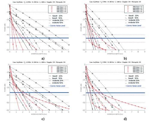
and the condition z > ∆ is assumed to be verified. As clearly seen in Fig. 8a, an IF of
about 12 dB can be obtained by this technique at large depths.
14scientific instruments
Fig. 8. Improvement Factor (IF) of the surface
clutter cancellation techniques. a: Doppler
filtering; b: dual-antenna cancellation (1° roll
angle and 10% antenna pattern knowledge
accuracy); c: dual-frequency cancellation as a
function of number of averaged looks.
Since surface clutter echoes from off-nadir in the cross-track direction are not
affected by any Doppler modulation and cannot be eliminated by the previous
technique, additional clutter suppression techniques were studied for MARSIS, based
on a dual-antenna or dual-frequency processing concept.
The dual-antenna cancellation technique (Picardi et al., 1998a; 1999a) uses a
primary antenna to transmit and receive the composite subsurface/surface signal, with
a pattern maximum in the nadir direction (for MARSIS, a dipole mounted parallel to
the surface and normal to the motion direction) and a secondary antenna to receive
surface clutter only, with a pattern null in the nadir direction (for MARSIS, a short
monopole oriented vertically under the spacecraft). The cancellation scheme is a
coherent subtraction after correction for the antenna gain imbalance between the two
channels:
G1 1u2
Vtot V1 V2
B G2 1u2
(10)
with V1 and V2 the complex signals at the dipole and monopole channels, and G1(θ)
and G2(θ) the antenna gain patterns for the dipole and monopole, respectively. It is
simple to show (Picardi et al., 1999a) that the surface clutter echoes are completely
removed by the subtraction, leading to infinite IF, if we assume that:
— returns from the two antennas are totally correlated;
— surface and subsurface return contributions to V1 and V2 are totally uncorrelated;
— the antenna patterns G1(θ) and G2(θ) are perfectly known;
— the monopole pattern null points exactly towards the nadir direction in both
along-track and cross-track directions;
— the primary and secondary antenna channels have the same phase/amplitude
transfer function (perfectly amplitude-balanced and phase-matched channels).
15SP-1240
Fig. 9. Ice/Water interface detection charts. In practice, the dual-antenna cancellation IF is limited by imperfect knowledge of
Subsurface attenuation (including absorption the antenna pattern, unknown antenna pointing errors (roll and pitch angles) and
and scattering loss) appears in black; surface amplitude/phase mismatching between the two channels. In Picardi et al. (1999a),
clutter after coherent cancellation in red; noise
floor in blue. Altitudes are H = 250 km and these effects were considered and it was concluded that the main limitation to the IF
800 km; frequencies are 1.8 MHz and 5 MHz. comes from the antenna pattern knowledge and the cross-track pointing error of the
Surface correlation length is 1000 m. monopole (roll angle).
Typical IF behaviour as a function of the antenna gain variance σg2 and the space-
craft roll angle α is shown in Fig. 8b. Values of 10% accuracy in the knowledge of the
antenna patterns and ±1° roll angle result in a maximum IF of about 20 dB. Note that
this clutter cancellation technique could also be performed on the square-law detected
signals on the two dipole and monopole channels, but with reduced performance.
Another technique for clutter suppression, based on non-coherent processing of
echoes acquired simultaneously at different frequencies, has been proposed (Picardi
et al., 1999a), in order to provide surface clutter cancellation if the dual-antenna
technique proves insufficient (for example, owing to problems in positioning the
monopole null) or cannot be applied because monopole channel data are not available
on the ground. The dual-frequency technique uses the fact that the surface clutter
16scientific instruments
power at two frequencies remains almost constant (or the changes can be easily Fig. 10. Dry/Ice interface detection charts.
predicted by modelling), while the subsurface power is a strong function of frequency. Subsurface attenuation (including absorption
and scattering loss) appears in black; surface
As consequence, if the detected signals at both frequencies are subtracted, the surface
clutter after coherent cancellation in red; noise
contribution is significantly reduced while the subsurface contribution remains floor in blue. Altitudes are H = 250 km and
unchanged. The main limitation of this technique arises from the speckle which 800 km; frequencies are 1.8 MHz and 5 MHz.
decorrelates at the two frequencies, and represents a clutter residual after cancellation. Surface correlation length is 1000 m.
If the mean powers of surface clutter at the two frequencies are assumed to be equal,
IF can be shown to be linearly related to the number of averaged looks before
subtraction of the signal (Picardi et al., 1999a). As clearly seen in Fig. 8c, an IF of
about 5 dB can be obtained using five averaged looks.
8.4 Subsurface return signal-to-noise performance
Figures 9-10 summarise the predicted performance of the radar sounder in detecting
the ice/water and dry/ice subsurface interfaces, according to the simple models
described above and using the nominal MARSIS design parameters discussed in
Section 6.1. Figure 9 refers to ice/water interface detection, and Fig. 10 to dry/ice.
The four graphs in each figure present the detection at the two boundary frequency
17SP-1240
bands (1.8 MHz and 5 MHz) from two altitudes (250 km and 800 km), which
represent the minimum and maximum heights of Mars Express during the portion of
the orbit when MARSIS is active. Each detection chart contains the following
normalised power levels as a function of the interface depth:
— subsurface return power, including effects of absorption and scattering. Absorption
is taken into account as in Section 8.1, assuming the two end-member host
materials (basalt and andesite) and porosities (20-50%). The backscattering is
computed assuming a subsurface correlation length equal to 2000 m and two
extreme values of the subsurface layer rms slope (1° and 5°);
— surface clutter power after coherent clutter cancellation, including Doppler
filtering and dual-antenna cancellation (dual-frequency cancellation is not
considered because we want to evaluate single-look performance). Two values of
rms slope are used, between 1° and 5°, while the surface correlation length is also
assumed to be 2000 m;
— noise floor level, computed to match the S/N values reported in Section 8.2, plus
a little increment from the receiver internal noise amplification after the dual-
antenna cancellation.
Based on a 0 dB detection threshold criterion, it is easily seen from the figure that,
thanks to the surface clutter cancellation techniques and to the strong noise
suppression, penetration depths to several kilometres can be achieved under the most
likely scenarios for the martian crust.
9. Ionospheric Sounding Since the ionosphere is a very good specular reflector, the S/N for active ionospheric
Performance sounding is expected to be good. The main difficulty is that, at frequencies below the
half-wavelength resonance of the antenna (~3 MHz), the radiated power decreases
rapidly with decreasing frequency (approximately as frequency to the fourth power).
This is compensated for to some extent by the fact that the range to the ionospheric
reflection point decreases with decreasing frequency (Fig. 2a), which tends to
improve the S/N at low frequencies. Also, at frequencies below ~1 MHz, the cosmic
noise background falls with decreasing frequency, which also improves the S/N at
low frequencies. At a spacecraft altitude of 500 km, the resulting S/N for the daytime
ionospheric model shown in Fig. 2a is expected to be 5.4 dB at 0.1 MHz, increasing
to 8.6 dB at 0.3 MHz, 18.4 dB at 1.0 MHz and 21.3 dB at 3.0 MHz. These S/Ns are
adequate to perform ionospheric sounding on the dayside of Mars under almost all
conditions. On the night side, where the electron densities are expected to be much
lower, the S/N is likely to become marginal, since the plasma frequencies are much
lower, which increases the range to the reflection point for any given spacecraft
altitude. It is also possible that the ionosphere may be more disturbed on the nightside
of Mars, which could cause scattering from small-scale irregularities, thereby causing
a further reduction in the S/N. Although the ionospheric sounding performance is
somewhat marginal on the nightside, it is almost certain that useful information will
be obtained, particularly at low altitudes where the range to the reflection point is very
small. Also, a very strong return signal is expected when the sounding frequency
passes through the local plasma frequency, which will give the local electron plasma
density under almost all conditions.
18scientific instruments
Biccari, D., Picardi, G., Seu, R. & Melacci, P.T. (2001a). Mars Surface Models and References
Subsurface Detection Performance in MARSIS. In Proc. IEEE International Symp.
on Geoscience and Remote Sensing, IGARSS 2001, Sydney, Australia, 9-13 July
2001.
Biccari, D., Ciabattoni, F., Picardi, G.,Seu, R., Johnson, W.K.T. Jordan, R., Plaut, J.,
Safaeinili, A., Gurnett, D.A., Orosei, R., Bombaci, O., Provvedi, F., Zampolini, E.
& Zelli, C. (2001b). Mars Advanced Radar for Subsurface and Ionosphere
Sounding (MARSIS). In Proc. 2001 International Conference on Radar, October
2001, Beijing, China.
Biccari, D., Cartacci, M., Lanza, P., Quattrociocchi, M., Picardi, G., Seu, R.,
Spanò, G. & Melacci, P.T. (2001c). Ionosphere Phase Dispersion Compensation,
Infocom Technical Report N.002/005/01-23/12/2001.
Carr, M.H. (1996). Water on Mars, Oxford University Press, Oxford, UK.
Fung, A.K. & Eom, H.J. (1983). Coherent Scattering of a Spherical Wave from an
Irregular Surface. IEEE Trans. on Antennas and Propagation, AP-31(1), 68-72.
Hanson, W.B., Sanatani, S. & Zuccaro, D.R. (1977). The Martian Ionosphere as
Observed by the Viking Retarding Potential Analyzers. J. Geophys. Res. 82, 4351-
4363.
Picardi, G. & Sorge, S. (1999). Adaptive Compensation of Mars Ionosphere
Dispersion: A Low Computational Cost Solution for MARSIS, Infocom Technical
Report MRS-002/005/99, October 1999.
Picardi, G., Plaut, J., Johnson, W., Borgarelli, L., Jordan, R., Gurnett, D., Sorge, S.,
Seu, R. & Orosei, R. (1998a). The Subsurface Sounding Radar Altimeter in the
Mars Express Mission, Proposal to ESA, Infocom document N188-23/2/1998,
February 1998.
Picardi, G., Sorge, S., Seu, R., Fedele, G., Federico, C. & Orosei, R. (1999a). Mars
Advanced Radar for Subsurface and Ionosphere Sounding (MARSIS): Models and
System Analysis, Infocom Technical Rep. MRS-001/005/99, March 1999.
Picardi, G., Sorge, S., Seu, R., Fedele, G. & Jordan, R.L. (1999b). Coherent Cancella-
tion of Surface Clutter Returns for Radar Sounding. In Proc. IEEE International
Symp. on Geoscience and Remote Sensing, IGARSS’99, Hamburg, Germany,
28 June - 2 July 1999, pp2678-2681.
Safaeinili, A. & Jordan, R.L. (2000). Low Frequency Radar Sounding through
Martian Ionosphere. In Proc. IGARSS 2000, 24-28 July 2000, Honolulu, Hawaii,
IEEE, pp987-990.
Stix, T.H. (1964). The Theory of Plasma Waves, McGraw-Hill, New York.
Zhang, M.H.G., Luhmann, J.G., Kliore, A.J. & Kim, J. (1990a). A Post-Pioneer
Venus Reassessment of the Martian Dayside Ionosphere as Observed by Radio
Occultation Methods. J. Geophys. Res. 95, 14,829-14,839.
Zhang, M.H.G., Luhmann, J.G., Kliore, A.J. & Kim, J. (1990b). An Observational
Study of the Nightside Ionospheres of Mars and Venus with Radio Occultation
Methods. J. Geophys. Res. 95, 17,095-17,102.
19You can also read