Micromagnetics of rare-earth efficient permanent magnets
←
→
Page content transcription
If your browser does not render page correctly, please read the page content below
Micromagnetics of rare-earth efficient permanent
                                                     magnets
arXiv:1903.11922v1 [cond-mat.mtrl-sci] 28 Mar 2019

                                                                    Johann Fischbacher1 , Alexander Kovacs1 , Markus
                                                                    Gusenbauer1 , Harald Oezelt1 , Lukas Exl2,3 , Simon Bance4 ,
                                                                    Thomas Schrefl1
                                                                    1 Department for Integrated Sensor Systems, Danube University Krems, Viktor
                                                                    Kaplan Straße 2, 2700 Wiener Neustadt, Austria
                                                                    2 Faculty of Mathematics, University of Vienna, Oskar-Morgenstern-Platz 1,

                                                                    1090 Wien, Austria
                                                                    3 Institute for Analysis and Scientific Computing, Vienna University of

                                                                    Technology, Wiedner Hauptstraße 8-10, 1040, Wien, Austria
                                                                    4 Seagate Technology, 1 Disc Drive, Springtown, Derry, BT48 0BF Northern

                                                                    Ireland, UK
                                                                    E-mail: thomas.schrefl@donau-uni.ac.at

                                                                    January 2018

                                                                    Abstract. The development of permanent magnets containing less or no rare-
                                                                    earth elements is linked to profound knowledge of the coercivity mechanism.
                                                                    Prerequisites for a promising permanent magnet material are a high spontaneous
                                                                    magnetization and a sufficiently high magnetic anisotropy. In addition to the
                                                                    intrinsic magnetic properties the microstructure of the magnet plays a significant
                                                                    role in establishing coercivity. The influence of the microstructure on coercivity,
                                                                    remanence, and energy density product can be understood by using micromagnetic
                                                                    simulations. With advances in computer hardware and numerical methods,
                                                                    hysteresis curves of magnets can be computed quickly so that the simulations
                                                                    can readily provide guidance for the development of permanent magnets. The
                                                                    potential of rare-earth reduced and free permanent magnets is investigated using
                                                                    micromagnetic simulations. The results show excellent hard magnetic properties
                                                                    can be achieved in grain boundary engineered NdFeB, rare-earth magnets with
                                                                    a ThMn12 structure, Co-based nano-wires, and L10 -FeNi provided that the
                                                                    magnet’s microstructure is optimized.

                                                     Keywords: micromagnetics, permanent magnets, rare earth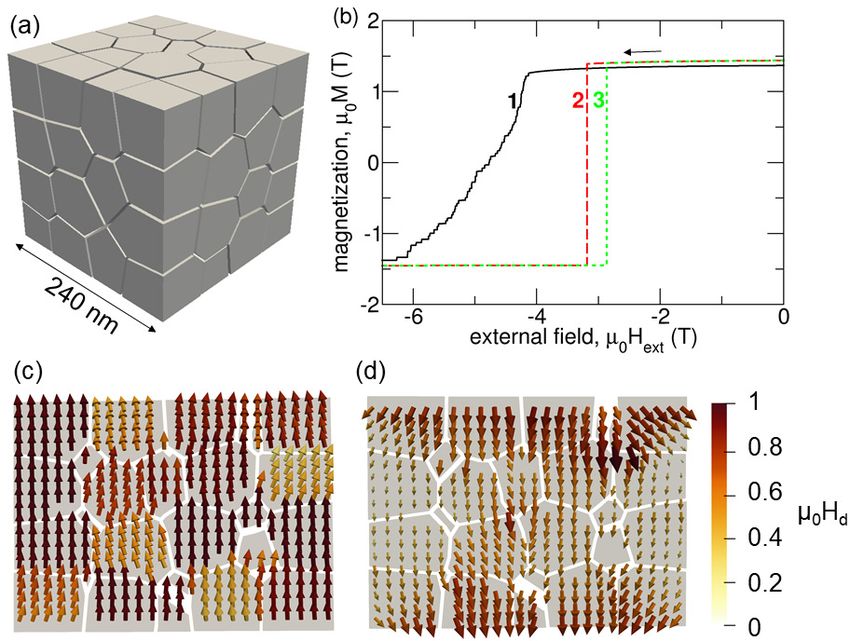
Micromagnetics of rare-earth efficient permanent magnets                                                              2

1. Introduction

1.1. Rare-earth reduced permanent magnets
High performance permanent magnets are a key tech-
nology for modern society. High performance mag-
nets are distinguished by (i) the high magnetic field
they can create and (ii) their high resistance to op-
posing magnetic fields. A prerequisite for these two
characteristics are proper intrinsic properties of the
magnet material: A high spontaneous magnetization
and high magneto-crystalline anisotropy. The inter-
metallic phase Nd2 Fe14 B [1, 2] fulfills these properties.   Figure 1. Usage of NdFeB magnets in the six major markets
Today NdFeB-based magnets dominate the high per-              in the year 2015. Data taken from [3].
formance magnet market. In the following we will use
“Nd2 Fe14 B” when we refer to the intermetallic phase
                                                              anisotropy field and the coercive field of Nd2 Fe14 B
and “NdFeB” when we refer to a magnet which is based
                                                              rapidly decays with increasing temperature. In order
on Nd2 Fe14 but contains additional elements. There
                                                              to compensate this loss, some of the magnet’s Nd is
are six major sectors which heavily rely on rare-earth
                                                              replaced with heavy rare earths such as Dy. Figure
permanent magnets [3]. The usage of NdFeB is sum-
                                                              2 compares the coercive field of conventional Dy-free
marized in figure 1 based on data given by Constan-
                                                              and Dy-containing NdFeB magnets as a function of
tinides [3] for 2015. Modern acoustic transducers use
                                                              temperature. (NdDy)FeB magnets, containing around
NdFeB magnets. Speakers are used in cell phones, con-
                                                              10 weight percent Dy, can reach coercive fields µ0 Hc >
sumer electronic devices, and cars. The total number
                                                              1 T at 450 K. However, since the rare-earth crisis [6] the
of cell phones that are shipped per year is reaching 2
                                                              rare-earth prices have become more volatile. During
billion. Air conditioning is a growing market. Around
                                                              2010 and 2011 the Dy price peaked and increased by
100 million units are shipped every year. Each unit
                                                              a factor of 20 [7]. Only four percent of the primary
uses about three motors with NdFeB magnets. Nd-
                                                              rare-earth production comes from outside China [6].
FeB magnets are essential to sustainable energy pro-
                                                              Because of supply risk and increasing demand, Nd and
duction and eco-friendly transport. The generator of a
                                                              Dy are considered to be critical elements [8]. In order
direct drive wind mill requires high performance mag-
                                                              to cope with the supply risk, magnet producers and
nets of 400 kg/MW power; and on average a hybrid
                                                              users aim for rare-earth free permanent magnets. With
and electric vehicle needs 1.25 kg of high end perma-
                                                              respect to the magnet’s performance, rare-earth free
nent magnets [4]. Another rapidly growing market is
                                                              permanent magnets may fill a gap between ferrites and
electric bikes with 33 million global sales in 2016. For a
                                                              NdFeB magnets [9]. An alternative goal is magnets
long time NdFeB magnets have been used in hard disk
                                                              with less rare earth than (NdDy)FeB magnets but
drives. Hard disk drives use bonded NdFeB magnets
                                                              comparable magnetic properties [10].
in the motor that spins the disk and sintered NdFeB
                                                                   Possible routes to achieve these goals are:
magnets for the voice coil motor that moves the arm.
There are around 400 million hard disk drives shipped           • Shape anisotropy based permanent magnets;
every year.                                                     • Grain boundary diffusion;
      In many applications the NdFeB magnet are used
                                                                • Improved grain boundary phases;
at elevated temperature. For example, the operating
temperature of the magnet in the motor/generator                • Nanocomposite magnets;
block of hybrid vehicles is at about 450 K. Though              • Alternative hard magnetic compounds.
Nd2 Fe14 B (Tc = 558 K) shows excellent properties            In this work we will use micromagnetic simulations,
at room temperature its Curie temperature Tc is               in order to address various design issues for rare-earth
much lower than those of SmCo5 (Tc = 1020 K) or               efficient permanent magnets. Micromagnetic simula-
Sm2 Co17 (Tc = 1190 K) magnets [5]. Therefore the             tions are an important tool to understand coercivity
Micromagnetics of rare-earth efficient permanent magnets                                                                     3

                                                             Figure 3. The maximum energy density product (BH)max is
                                                             given by the area of the largest rectangle that fits below the 2nd
                                                             quadrant of the B(H) curve. Left: M (H) loop, right: B(H)
                                                             loop of an ideal magnet.
Figure    2.          Coercive field of Nd15 Fe77 B8 and
(Nd0.77 Dy0.33 )15 Fe77 B8 magnets as function of tempera-
ture. Data taken from [17].                                  the magnetic field H by a uniform vectorR field inside
                                                             the magnet, we can write Emag,a = (1/2) Vi (BH)dV ,
mechanisms in permanent magnets. With the advance            where B = |B| and H = |H|. We see that we can
of hardware for parallel computing [11–13] and the im-       increase the energy stored in its external field either
provement of numerical methods [14–16], micromag-            by increasing the magnet’s volume Vi or by increasing
netic simulations can take into account the microstruc-      the product (BH), which is referred to as energy
ture of the magnet and thus help to understand how           density product [19]. It is defined as the product
the interplay between intrinsic magnetic properties and      of the magnetic induction B and the corresponding
microstructure impacts coercivity.                           opposing magnetic field H [20] and is given in units
                                                             of J/m3 . When there are no field generating currents,
                                                             the magnetic field inside the magnet
1.2. Key properties of permanent magnets
                                                             H = −N M                                                      (3)
The primary goal of a permanent magnet is to create
a magnetic field in the air gap of a magnetic circuit.       depends on the magnet’s shape which can be expressed
The energy stored in the field outside of a permanent        by the demagnetizing factor N . We further assume
magnet can be related to its magnetization and to its        that the magnet is saturated and there are no
shape. According to Maxwell’s equations the magnetic         secondary phases so that |M| = Ms , where Ms is
induction B is divergence-free (solenoidal): ∇ · B =         the spontaneous magnetization of the material. Using
0 and in the absence of any current the magnetic             equations (1) and (3) we express the energy density
field H is curl-free (irrotational): ∇ × H = 0. The          product as (BH) = |µ0 (M − N M)| |−N M| = µ0 (1 −
volume integral of the product of a solenoidal and           N )N Ms2 [9, 21]. When maximized with respect to N
irrotational vector field over all space is zero, when the   this gives the maximum energy density product of a
corresponding vector and scalar potentials are regular       given material
at infinity [18]. This is the case when                                   1
                                                             (BH)max = µ0 Ms2                                     (4)
B = µ0 (M + H)                                        (1)                 4
                                                             for N = 1/2. It is worth to check the shape of a
is the magnetic induction due to the magnetization
                                                             magnet with a demagnetizing factor of 1/2. Let us
M of a magnet. Here µ0 = 4π × 10−7 Tm/A is the
                                                             assume a magnet in form of a prism with dimensions
permeability of vacuum. The magnetostatic energy in
                                                             l × l × pl which is magnetized along the edge with
a volume Va of free Rspace, where M = 0 and B = µ0 H,
                                                             length pl. Then a simple approximate equation for the
 is Emag,a = (µ0 /2) Va H2 dV . Splitting the space into
                                                             demagnetizing factor is N = 1/(2p+1) [22]. Therefore,
Rthe volume inside   the magnet,  Vi , and Va , we have
                                                             the optimum shape of a magnet that results in the
   B · HdV = Va µ0 H2 dV + Vi B · HdV = 0 or
              R               R
                                                             maximum energy density product is a flat prism with
                                                             dimensions l × l × 0.5l, which is twice as wide as high.
              Z
            1
 Emag,a = −       B · HdV.                           (2)     Many modern magnets have this shape.
            2 Vi
                                                                  When there is no drop of the magnetization with
Since the left-hand side of equation (2) is positive, B
                                                             increasing opposing field until H > Ms /2, the energy
and H must point in opposite directions inside the
                                                             density product reaches its maximum value given by
magnet. Approximating the magnetic induction B and
                                                             equation (4). In this case, the magnetic induction B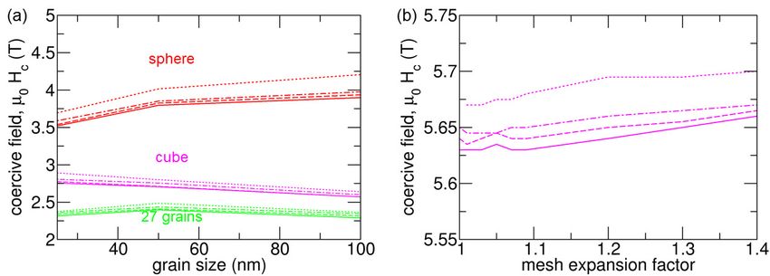
Micromagnetics of rare-earth efficient permanent magnets                                                               4

as function of field is a straight line. For an ideal loop
as shown in figure 3 the remanent magnetization, Mr ,
equals the spontaneous magnetization, Ms . In some
materials, magnetization reversal may occur at fields
lower than half the remanence. When Hc < Mr /2, the
energy density product is limited by the coercive field,
Hc . Similarly, the maximum value for (BH)max is not
reached, when M (H) is not square but decreases with
increasing field H.
     A higher energy density product reduces volume
and weight of the permanent-magnet-containing device
making it an important figure of merit. Other decisive
                                                             Figure 4. Both the intrinsic magnetic properties and the
properties are the remanence, the coercive field, and        physical/chemical structure of the magnet determine coercive
the loop squareness.                                         field, remanence and energy density product.

1.3. Permanent magnets and intrinsic magnetic
                                                             are one reason for the reduction of the coercive field
properties
                                                             with respect to its ideal value. In the presence of
A magnetic material suitable for a permanent magnet          defects with zero magnetocrystalline anisotropy, the
must have certain intrinsic magnetic properties. From        coercive field may reduce to Hc = HN /4. Plugging
inspection of figure 3 we see that a good permanent          this limit for the coercive field into equation (5) gives
magnet material requires a high spontaneous magneti-         the condition K > µ0 Ms2 for the anisotropy constant.
zation Ms and a uniaxial anisotropy constant K that          This corresponds to the empirical law κ > 1 for many
creates a coercive field                                     hard magnetic p  phases of common permanent magnets
      Ms                                                     [9], where κ = K/(µ0 Ms2 ) is the hardness parameter
Hc >      .                                        (5)       [28].
       2
The theoretical maximum for the coercive field is the              The key figures of merit of permanent magnets
nucleation field [23]                                        such as the coercive field, the remanence, and
                                                             the energy density product are extrinsic properties.
         2K
HN =                                               (6)       They follow from the interplay of intrinsic magnetic
        µ0 Ms                                                properties and the granular structure of the magnet
for magnetization reversal by uniform rotation of a          which is schematically shown in figure 4. Thus,
small sphere. Equations (5) and (6) give the condition       in addition to the spontaneous magnetization Ms ,
K > µ0 Ms2 /4.      In other words, the anisotropy           magnetocrystalline anisotropy constant K, and the
energy density, K, should be larger than the maximum         exchange constant A, a well-defined physical and
energy density product, (BH)max . For most magnetic          chemical structure of the magnet is essential for
materials this condition is not sufficient [9]. There        excellent permanent-magnet properties.
are two stronger conditions for the magnetocrystalline             Empirically, the effects that reduce the coercive
anisotropy constant.                                         field with respect to the ideal nucleation field are often
      To be able to make a permanent magnet or its           written as [29, 30]
constituents in any shape, the nucleation field must
                                                             Hc = αK αψ HN − Neff Ms − Hf .                          (7)
be higher than the maximum possible demagnetizing
field. The demagnetizing factor of a thin magnet             The coefficients αK and αψ express the reduction
approaches 1 and the magnitude of the demagnetizing          in coercivity due to defects and misorientation,
field approaches Ms which gives the condition K >            respectively [31]. The microstructural parameter Neff
µ0 Ms2 /2. This is often expressed in terms of the           is related to the effect of the local demagnetization
quality factor Q = 2K/(µ0 Ms2 ), which was introduced        field near sharp edges and corners of the microstructure
in the context of bubble domains in thin films [24,          [32]. The fluctuation field Hf gives the reduction of the
25]. For Q > 1 stable domains are formed and                 coercive field by thermal fluctuations [33].
the magnetization points either up or down along                   Let us look at an example. Figure 5a shows
the anisotropy axis perpendicular to the film plane.         the microstructure of a nanocrystalline Nd2 Fe14 B
Otherwise, the demagnetizing field would cause the           magnet used for micromagnetic simulations to identify
magnetization to lie in plane.                               the different effects that reduce coercivity. For the
      The maximum possible coercive field is never           set of material parameters used (K = 4.3 MJ/m3 ,
reached experimentally. This phenomenon is usually           µ0 Ms = 1.61 T, A = 7.7 pJ/m), the ideal
referred to as Brown’s paradox [26, 27]. Imperfections       nucleation field is µ0 HN = 6.7 T. The 64 grains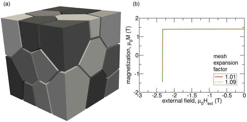
Micromagnetics of rare-earth efficient permanent magnets 5
boundary phase. The magnetostatic terms are not
taken into account. The grain boundary phase acts
as a soft magnetic defect and reduces coercivity. The
corresponding microstructural parameter is αK = 0.67.
Owing to exchange coupling between the grains all
grains reverse at the same external field. For the
dotted line (case 3) we switch on the demagnetizing
field. The magnetization and the demagnetizing field
are shown in a slice through the grains in figures 5c and
5d, respectively. The reduction of the coercive field
owing to demagnetizing effects equates to Neff = 0.2.
Finally, we take into account thermal activation by
computing the energy barrier for the nucleation of
reversed domains as function of field [38]. The decrease
of coercivity by thermal activation is µ0 Hf = 0.23 T.
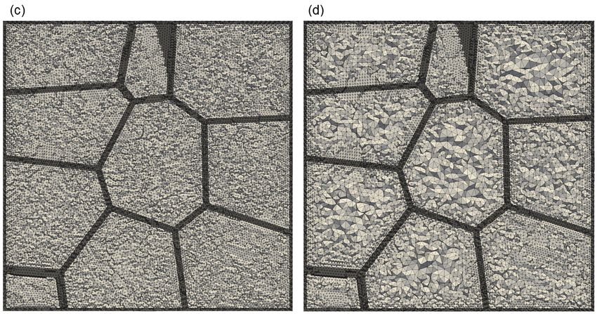
Figure 5. (a) Microstructure used for the simulation of mi-
crostructural effects that decrease the coercive field. (b) 1 mis-
2. Micromagnetics of permanent magnets
alignment (solid line) : non-magnetic grain boundary phase, de-
magnetizing field switched off; 2 Defects(dashed line): Weakly
ferromagnetic grain boundary phase and demagnetization field 2.1. Micromagnetic energy contributions
switched off; 3 Demagnetizing effects: Weakly ferromagnetic
grain boundary phase and demagnetization field switched on. Micromagnetism is a continuum theory that handles
The vector fields in (c) and (d) show magnetization and the de- magnetization processes on a length scale that is small
magnetizing field before switching for case 3. enough to resolve the transition of the magnetization
within domain walls but large enough to replace the
atomic magnetic moments by a continuous function of
were generated from a centroid Voronoi tessellation
position [39]. The state of the magnet is described
[34]. The average grain size was 60 nm. The
by the magnetization M, whose magnitude |M| =
anisotropy directions were randomly distributed within
Ms is constant and whose direction m = M/Ms is
a cone with an opening angle of 15 degrees. The
continuous. A stable or metastable magnetic state can
grain boundary phase of NdFeB magnets contains
be found by finding a function m = m(r) with |m| = 1
Fe and is weakly ferromagnetic [35–37]. In addition
that minimizes the Gibbs free energy of the magnet
to magnetostatic interactions between the grains, the Z h
grains are also weakly exchange coupled. In our E(m) =
2 2
A (∇mx ) + (∇my ) + (∇mz )
2
(8)
simulations the grain boundary phase was 3 nm thick. V
The magnetocrystalline anisotropy constant K of the 2
− K (m · k) (9)
grain boundary phase was zero. Its magnetization µ0 Ms
and exchange constant were µ0 Ms = 0.5 T and A = − (m · Hd ) (10)
2
7.7 pJ/m for cases 2 to 4. i
In numerical micromagnetics we can artificially − µ0 Ms (m · Hext ) dV. (11)
switch physical effects on or off and thus gain The different lines describe the exchange energy, the
a deeper understanding of how the various effects magnetocrystalline anisotropy energy, the magneto-
impact magnetization reversal. We start with the static energy, and the Zeeman energy, respectively.
granular system whereby the grains are separated The coefficients A, K, and Ms in equation (8) to
by a nonmagnetic grain boundary phase and the (11) vary with position and thus represent the mi-
magnetostatic energy term is switched off. Thus, crostructure of the magnet. The unit vector along the
there are no demagnetizing fields and no magnetostatic anisotropy direction, k, varies from grain to grain re-
interactions. The grains are isolated and there are flecting the orientation of the grains. The anisotropy
no defects. The solid line (case 1) of figure 5b constant K will be zero in local defects or within the
shows the influence of misalignment on magnetization grain boundary phase. The grain boundary phase may
reversal. Owing to the different easy directions the be weakly ferromagnetic with magnetization Ms and
grains switch at slightly different values of the external the exchange constant A considerably reduced with re-
field. The coercive field is µ0 Hc = 4.77 T. With spect to the bulk values. In α-Fe inclusions K is neg-
αK = 1, Neff = 0, and Hf = 0 which hold for ligible and Ms and A are high. Composite magnets
case 1 per definition, we obtain αψ = 0.71 from combine grains with different intrinsic properties. The
equation (7). For the computation of the dashed demagnetizing field Hd arises from the divergence of
line (case 2) we assume a weakly ferromagnetic grain the magnetization. The factor 1/2 in equation (10)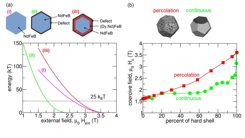
Micromagnetics of rare-earth efficient permanent magnets                                                             6

indicates that it is a self-energy which depends on the         Each node of a finite element mesh or cell of
current state of M. It can be calculated from the static   a finite difference scheme with index i holds a unit
Maxwell’s equations. One common method is the nu-          magnetization vector mi . We gather these vectors into
merical solution of the magnetostatic boundary value       the vector x which has the dimension 3n, where n is the
problem for the magnetic scalar potential U where the      number of nodes or cells. Then the Gibbs free energy
demagnetizing field is derived as Hd = −∇U . The           may be written as [14]
magnetic scalar potential fulfills the Poisson equation             1           µ0 T
                                                           E(x) = xT Cx −          h M̄x − µ0 hT    ext M̄x.       (16)
∇2 U = ∇ · M                                       (12)             2            2 d
                                                           The three terms on the right-hand side of (16) from left
inside the magnet, the Laplace equation                    to right are the sum of the exchange and anisotropy
∇2 U = 0                                           (13)    energy, the magnetostatic self-energy, and the Zeeman
                                                           energy, respectively. The sparse matrix C contains
outside the magnet, and the interface conditions
                                                           grid information associated with the discretization of
U (in) = U (out)                                   (14)    the exchange and anisotropy energy. The matrix

  U (in) − U (out) · n = M · n                     (15)    M̄ accounts for the local variation of the saturation
                                                           magnetization Ms within the magnet. It is a diagonal
at the magnet’s boundary with unit surface normal          matrix whose entries are the modulus of the magnetic
n. Equation (14) follows from the continuity of the        moment associated with the node or cell i [14]. The
component of the magnetic field H parallel to the          vectors x, hd (x), and hext hold the unit vectors of
surface (which follows from ∇ × H = 0). Equation           the magnetization, the demagnetizing field, and the
(15) follows from the continuity of the component of       external field at the nodes of the finite element mesh
the magnetic induction B normal to the surface (which      or the cells of a finite difference grid, respectively.
follows from ∇ · B = 0) [40].                                   For computing the demagnetizating field, equa-
                                                           tions (12) to (15) can be solved using an algebraic
2.2. Numerical methods                                     multigrid method on the finite element mesh [14, 44,
                                                           45].
2.2.1. Hysteresis There is no unique constrained                In finite difference methods the magnetization
minimum for equation (8) to (11) for a given               is assumed to be uniform within each cell. Then
external field. The magnetic state that a magnet           the magnetic field generated at point r by the
can access depends on its history. Hysteresis in a         magnetization in cell j is given by an integration over
non-linear system results from the path formed by          the magnetic surface charges σj = Msj mj · n [46],
subsequent local minima [41]. In permanent magnet                                                   !
                                                                                          σj0
                                                                                 Z
studies we are interested in the demagnetization                          1                       0
                                                           Hd,j (r) = − ∇                     0
                                                                                                dSj ,              (17)
curve. Thus, we use the saturated state as initial                       4π       ∂Vj |r − r |
state and compute subsequent energy minima for a           where n is the unit surface normal. The magnetostatic
decreasing applied field, Hext . The projection of         energy is a double sum over all computational cells
the magnetization onto the direction of the applied                                 Z X
                                                                    µ0 X
field integrated over the volume of the magnet,            Em = −         Ms,i mi ·       Hd,j (r)dV.        (18)
         R
that is V Ms (m · Hext / |Hext |) dV , as function of               2 i              Vi j

different values of Hext gives the M (Hext )-curve.        Applying integration by parts we can rewrite the
For computing the maximum energy density product           magnetosatic energy as [47]
we need the M (H)-curve, where H is the internal                        Z Z
                                                                                   σi σj0
                                                                 µ0 X
field H = Hext − N M (Hext ).         Similar to open      Em =                           dS 0 dSi .   (19)
circuit measurements [42] we correct M (Hext ) with the          8π i,j ∂Vi ∂Vj |r − r0 | j
macroscopic demagnetizing factor N of the sample, in       Introducing the demagnetization tensor Nij reduces
order to obtain M (H).                                     equation (19) to
                                                                 µ0       X
                                                           Em =     Vcell     Msi mi Nij Msj mj ,        (20)
2.2.2. Finite element and finite difference discretiza-           2       i,j
tion The computation of the energy for a permanent
magnet requires the discretization of equations (8) to     where Vcell is the volume of a computational cell.
(11) taking into account the local variation of Ms , K,    The term µ0 Vcell Msi mi Nij Msj mj is the magnetostatic
and A, according to the microstructure. Common dis-        interaction energy between cells i and j. From equation
cretization schemes used in micromagnetics for perma-      (20) we can compute the cell averaged demagnetizing
nent magnets [43] are the finite difference method [13]    field [48, 49]
                                                                    X
or the finite element method [14, 15].                     hi = −       Nij Msj mj .                           (21)
                                                                    j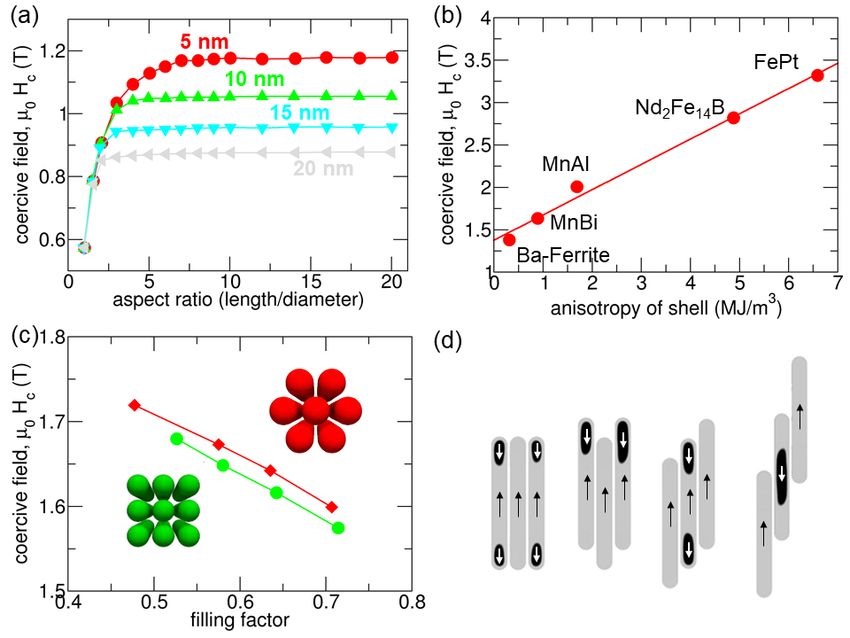
Micromagnetics of rare-earth efficient permanent magnets                                                            7

The demagnetization tensor Nij depends only on the           superscript + marks quantities which are computed
relative distance between the cells i and j. The             for the next iteration step. The superscript − marks
convolution (21) can be efficiently computed using           quantities which have been computed during the
Fast Fourier Transforms. Special implementations of          previous iteration step.
the Fast Fourier Transform with low communication
overhead makes large-scale simulations of permanent          Algorithm 1 minimize E(x)
magnets possible on supercomputers with thousands             repeat
of cores [13].                                                   compute search direction d
                                                                 compute step length α
2.2.3. Energy minimization The intrinsic time scale              proceed x+ = x + αd
of magnetization processes is related to the Lamor            until convergence
frequency f = γµ0 H/(2π). The gyromagnetic ratio is
γ = 1.76086 × 10¹¹ /(Ts). For example, let us estimate            Variants of the steepest-descent method, [11, 52–
the intrinsic time scale for precession in Nd2 Fe14 B. The   54], the non-linear conjugate gradient method [14,
magnitude of typical internal fields, µ0 H are about         15], and the quasi-Newton method [55–57] are most
a few Tesla. The Lamor frequency is 28 GHz per               widely used in micromagnetics for permanent magnets.
Tesla. This gives a characteristic time scale smaller        In steepest-descent methods the search direction is
than 10−10 s. Such time scales may be relevant               the negative gradient g = ∇E(x) of the energy:
for magnetic recording or spin electronic devices. In        d = −g. The nonlinear conjugate-gradient method
permanent magnet applications the rate of change of          uses a sequence of conjugate directions d = −g +
the external field is much slower. For example, low          βd− . The Newton method uses the negative gradient
speed direct drive wind mills run at about 20 rpm            multiplied by the inverse of the Hessian matrix: d =
[50] and motors of hybrid vehicles run at 1500 rpm to        −(∇2 E)−1 ∇g as search direction. In quasi-Newton
6000 rpm [51], which translate into frequencies ranging      methods the inverse of the Hessian is approximated
from 1/3 Hz to 100 Hz. The magnetization always              by information gathered from previous iterations.
reaches metastable equilibrium before a significant               The step length α is obtained by approximate line
change of the external field. Based on this argument         search minimization. To that end the new point is
many researchers use energy minimization methods             determined along the line defined by the current search
for simulation of magnetization reversal in permanent        direction and should yield a sufficiently smaller energy
magnets, taking advantage of a significant speedup as        with a sufficiently small gradient (approximate local
compared to time integration solvers [11, 15].               minimum along the line). By expanding and shrinking
       Minimizing equation (16) subject to the unit          a search interval for α, line search algorithms [58] find
norm constraint for decreasing external field gives the      an appropriate step length. Owing to the solution
magnetic states along the demagnetization curve of the       of the magnetostatic subproblem, evaluations of the
magnet. The sparse matrix C and the diagonal matrix          energy are expensive. In order to reduce the number
M̄ depend only on the geometry and the intrinsic             of energy evaluations Koehler and Fredkin [59] apply
magnetic properties. The vector hd depends linearly          an inexact line search based on cubic interpolation.
on the magnetization. Evaluation of the energy,              Tanaka and co-workers [15] propose to interpolate the
its gradient, or the Hessian requires the solution of        magnetostatic field within the search interval if it is
the magnetostatic subproblem. The magnetic field             sufficiently small. Fischbacher et al. [14] showed that
depends linearly on the magnetization. Thus, (16)            long steps should be avoided, in order to compute
is quadratic in x. However, the condition M = Ms             all metastable states along the demagnetization curve.
implies that each subvector mi of x is constrained           They suggest applying a single Newton step in one
to be a unit vector. The optimization problem is             dimension to get an initial estimate for the step
supplemented by n nonlinear constraints |mi | = 1, i =       length which then may be further reduced to fulfill
1, ..., n.                                                   the sufficient decrease condition. For steepest descent
       In its most simple form an algorithm for energy       methods Barzilai and Borwein [60] proposed a step
minimization (see algorithm 1) is an iterative process       length α such that α multiplied with the identity
with the following four tasks per iteration: The             matrix, 1, approximates the inverse of the Hessian
computation of the search direction, the computation         matrix: α1 ≈ (∇2 E)−1 . Thus, the Barzilai-Borwein
of the step length, the motion towards the minimum,          method makes use of the key idea of limited memory
and the check for convergence. These computations            quasi Newton methods applied to step length selection.
make use of the objective function E(x) and its              The step length is computed from information gathered
gradients, possibly second derivatives and maybe             during the last 2 iteration steps. This method was
information gathered from previous iterations. The           successfully applied in numerical micromagnetics [11,
Micromagnetics of rare-earth efficient permanent magnets 8
61, 62]. 2.2.4. Time integration The torque on the magnetic
When applied to micromagnetics the update rule moment MVcell of a computational cell in a magnetic
x+ = x + αd will not preserve the norm of the field H is T = µ0 MVcell × H. The angular
magnetization vector. A simple cure is renormalization momentum associated with the magnetic moment
m+ i = (mi + αdi )/ |(mi + αdi )|. When certain is L = −MVcell / |γ|. The change of the angular
conditions for d [63] and the computational grid [64] momentum with time equals the torque, ∂L/∂t = T.
are met the normalization leads to a decrease in the Applying the torque equation for the magnetic volume
energy. One condition [63] for an energy decrease which is divided into computational cells gives
upon normalization is that the search direction is ∂mi
perpendicular to the magnetic state of the current = − |γ| µ0 mi × heffi , (24)
∂t
point: mi · di for all i. Following Cohen et al. [65] we which describes the precession of the magnetic moment
can replace the energy gradient by its projection onto around the effective field. In order to describe the
its component perpendicular to the local magnetization motion of the magnetization towards equilibrium,
ĝi = gi − (gi · mi ) mi = −mi × (mi × gi ) . (22) equation (24) has to be augmented with a damping
term. Following Landau and Lifshitz [68] we can add
In nonlinear conjugate gradient methods the search di- a term −λmi × (mi × heffi ) to the right-hand side
rections are linear combinations of vectors perpendic- of equation (24) which will move the magnetization
ular to the magnetization (the current projected gra- towards the field. Alternatively we can - as suggested
dient and the previous search directions initially being by Gilbert [70] - add a dissipative force −α∂mi /∂t
the projected gradient). Instead of updating and nor- to the effective field. The precise path the system
malization, the vectors mi might also be rotated by follows towards equilibrium depends on the type of
an angle α |di | [66] or a norm conserving semi-implicit equation used and the value of the damping parameters
update rule [67] may be applied. λ or α. In the Landau-Lifshitz equation precession is
The right-hand side of equation (22) follows from not changed with increasing damping, whereas in the
the vector identity a×(b × c) = (a · c) b−(a · b) c and Gilbert case an increase of the damping constant slows
|mi | = 1. On computational grids with a uniform mesh down precessional motion. Only for small damping the
the energy gradient is proportional to the effective field Landau Lifshitz equation and the Gilbert equation are
1 equivalent. This can be seen if the Gilbert equation is
heffi = − gi . (23)
µ0 Msi Vcell written in Landau-Lifshitz form [71]
By inspecting the right-hand side of equation (22), ∂mi |γ| µ0
= − mi × heffi
we see that the search direction of a steepest-descent ∂t 1 + α2
method is proportional to the damping term of |γ| µ0
the Landau-Lifshitz equation [68]. Time integration −α mi × (mi × heffi ) . (25)
1 + α2
of the Landau-Lifshitz-Gilbert equation without the In the limit of high damping only the second term of
precession term [52] is equivalent to minimization by equation (25) remains and the time integration of the
the steepest-descent method. Furaya et al. [52] use Landau-Lifshitz-Gilbert equation becomes equivalent
a semi-implicit time integration scheme. They split to the steepest-descent method. For coherent rotation
the effective field into its local part and the long- of the magnetization the minimum reversal time occurs
ranging magnetostatic field which not only depends on for a damping parameter α = 1. In turn, fast
the nearest neighbor cells but on the magnetization reversal reduces the total computation time. This
in the entire magnet. By treating the local part is the motivation for using a damping parameter
of the effective field implicitly and the magnetostatic α = 1 for simulation of magnetization reversal in
field explicitly, much larger time steps and thus faster permanent magnets [66, 72] by numerical integration
convergence toward the energy minimum is possible. of equation (25). Several public domain micromagnetic
There are several possible termination criteria software tools use solvers for the numerical solution of
for a minimization algorithm. Koehler and Fredkin equation(25) based on the adaptive Euler methods [73],
[59] used the relative change in the energy between Runge-Kutta schemes [62], backward-differentiation
subsequent iterations. Others [13, 52] use the difference methods [74], and preconditioned implicit solvers [75].
between the subsequent magnetic states. Gill et al. [69]
recommend a threefold criterion taking into account
2.2.5. Energy barriers Permanent magnets are used
the change in energy, the change in the magnetic
at elevated temperature. However, classical micromag-
state, and the norm of the gradient for unconstrained
netic simulations take into account temperature only
optimization. This ensures convergence of the sequence
by the temperature-dependent intrinsic materials prop-
of the magnetic states, avoids early stops in flat regions
erties. Thermal fluctuations that may drive the sys-
and ensures progress towards the minimum.
tem over a finite energy barrier are neglected. BeforeMicromagnetics of rare-earth efficient permanent magnets 9
Figure 7. Thermally induced magnetization reversal in a
Nd2 Fe14 B cube. Left: Computed demagnetization curve
by classical micromagnetics. Right: Energy barrier for the
formation of a reversed nucleus as a function of the applied
Figure 6. Energy landscape as function of the magnetization field. The inset shows the saddle point configuration of the
angle. (a) Small hard magnetic sphere in an external field. The magnetization. Data taken from [30].
field is applied at an angle of π − ψ = 45 degrees. (b) to (d)
With increasing field the energy barrier decreases.
compute the minimum energy path that connects the
local minimum at field Hext with the reversed magnetic
magnetization reversal, a magnet is in a metastable
state. A path is called a minimum energy path if for
state. With increasing opposing field the energy bar-
any point along the path the gradient of the energy is
rier decreases. The system follows the local minima
parallel to the path. In other words, the component
reversibly until the energy barrier vanishes and the
of the energy gradient normal to the path is zero.
magnetization changes irreversibly [76]. If the height
The string method can be easily applied by subsequent
of the energy barrier is around 25kB T , thermal fluc-
application of a standard micromagnetic solver. It is
tuations can drive the system over the barrier within
an iterative algorithm: The magnetic states along the
a time of approximately one second [77]. To illus-
path are described by images. Each image is a replica
trate this behavior, let us look at the energy land-
of the total system. A single iteration step consists
scape of a small hard magnetic sphere with volume
of two moves. (1) Each image is relaxed by applying
V (see figure 6). The energy per unit volume is
a few steps of an energy minimization method or by
E(ϕ, Hext )/V = K sin2 (ϕ)−µ0 Ms Hext cos(ϕ−ψ). The
integrating the Landau-Lifshitz-Gilbert equation for
external field is applied at an angle ψ with respect to
a very short time. (2) The images are moved along
the positive anisotropy axes. For small external fields
the path such that the distance between the images is
the energy shows two minima as function of the magne-
constant. Within the framework of the elastic band
tization angle ϕ. The state before switching is given by
method images may only move perpendicular to the
ϕ1 = (π−ψ)Ms Hext /(2K −Ms Hext ) and the state after
current path and the distance between the images
switching is given by ϕ2 = π − (π − ψ)Ms Hext /(2K +
is kept constant with a virtual spring force. For
Ms Hext ). The√maximum energy occurs at the saddle
an accurate computation of the energy barrier for a
point at ϕ0 = 3 − tan ψ [78].
nucleation process [83] variants of the string method
In permanent magnets magnetization reversal
exists which keep more images next to the saddle point.
occurs by the nucleation and expansion of reversed
This can be achieved by an energy weighted distance
domains [79]. Similar to the situation depicted in
function between the images [84] and truncation of the
figure 6 the nucleation of a reversed domain or the
path [85].
depinning of a domain wall is associated with an
Figure 7 compares the coercive field of a Nd2 Fe14 B
energy barrier that is decreased by an increasing
cube with an edge length of 40 nm obtained by
external field. Using the elastic band method [80]
classical micromagnetic simulations and computing
or the string method [81] the energy barrier can be
energy barriers as discussed above. In both methods
computed as function of the external field. The
the intrinsic magnetic material parameters for T =
critical field at which the energy barrier EB (Hext )
300 K were used. The non-zero temperature coercive
crosses the 25kB T -line is the coercive field of the
field, which takes into account thermal fluctuations,
magnet taking into account thermal fluctuations. The
is defined as the critical value of the external field
elastic band method and the string method are well-
at which the energy barrier reaches 25kB T . By
established path finding methods in chemical physics
inspecting the magnetic states along the minimum
[82, 83]. In micromagnetics they can be used to
energy path we can see how thermally inducedMicromagnetics of rare-earth efficient permanent magnets 10
magnetization reversal happens. At the saddle point
a small reversed nucleus is formed. If there is no
barrier for the expansion of the reversed domain, the
reversed domain grows and the particle will switch.
The simulations are self-consistent: The coercive field
calculated by classical micromagnetics equals the field
at which the energy barrier vanishes. For nearly ideal
particles such as the cube without soft magnetic defects
Figure 8. (a) Coercive field of a sphere, a cube, and a
discussed above, the reduction of the coercive field by polycrystalline magnet as function of grain size. The grains are
thermal fluctuations may be as large as 25 percent made of Nd2 F14 B and surrounded by a 3 nm thick, weakly-
[86]. However, the presence of defects reduces the ferromagnetic
p grain boundary phase. The grain size is defined
decay of coercivity owing to thermal fluctuations [30]. as 3 Vgrain , where Vgrain is the volume of the grain. (b) Coercive
For example for the magnetic structure in figure 2, field of the 100 nm pure Nd2 F14 B cube as function of the
expansion factor a in a geometrical mesh. The solid, dashed,
which contains a weakly ferromagnetic grain boundary, dot-dashed, and dotted line refer to a mesh size of 1.3 nm, 2 nm,
thermal fluctuations reduce the coercive field by only 2.7 nm, and 4 nm, respectively, defined at the surface of the
8 percent. cube.
Energy barriers for reversal may also be computed
by atomstic spin dynamics. Miyashita et al. [87, 88]
nucleus from the rest, to be known with high accuracy.
solved equation (25) numerically for atomic magnetic
Therefore, we should be able to resolve the transition
moments augmented by a stochastic thermal field.
of the magnetization within the domain wall on the
From the computed relaxation time, τ , at a fixed
computational grid. The width of a Bloch p wall is
external field the energy barrier can be computed
δB = πδ0 . The Bloch wall parameter δ0 = A/K
by fitting the results to an Arrhenius-Neel law τ =
denotes the relative importance of the exchange energy
(1/f0 ) exp(EB /(kB T )) or to Sharrock’s law [89], which
versus crystalline anisotropy energy.
gives the coercive field as function of Hext and τ .
Whereas in ellipsoidal particles the demagnetizing
Alternatively, Toga et al. used the constrained Monte-
field is uniform, it is inhomogeneous in polyhedral
Carlo method [90] to compute field dependent energy
particles. The non-uniformity of the demagnetizing
barriers for an atomistic spin model.
field strongly influence magnetization reversal [94].
In equation (7) we attributed the reduction of co-
Near edges or corners [32] the transverse component of
ercivity to the fluctuation field Hf . The energy barrier
the demagnetizing field diverges. Owing to the locally
for magnetization reversal is related to this fluctuation
increased demagnetizing field, the reversed nucleus
field by Hf = −25kB T /(∂E/∂Hext ). Experimentally,
will form near edges or corners [95] (see also figure
the energy barrier or the fluctuation field can be ob-
7). We have to correctly resolve the rotations of
tained by measuring the magnetic viscosity which is
the magnetization that eventually form the reversed
related to the change of magnetization with time at a
nucleus. For the computation of the nucleation field
fixed external field. It was measured by Givord et al.
the required minimum mesh size p has to be smaller
[91], Villas-Boas [92], and Okamota et al. [93] for sin-
than the exchange length lex = A/(µ0 Ms2 /2) at the
tered, melt-spun, and hot-deformed magnets, respec-
place where the initial nucleus is formed. It gives
tively.
the relative importance of the exchange energy versus
magnetostatic energy. Please note that sometimes the
2.3. Microstructure representation
p
exchange length is also defined as llex = A/(µ0 Ms2 )
2.3.1. Grain size and particle shape The discretiza- [5, 96]. In order to keep the computation time low and
tion of the Gibb’s free energy by finite differences or resolve important magnetization processes, Schmidts
finite elements poses a question concerning the required and Kronmüller introduced a graded mesh that is
grid size. The required grid size is related to the char- refined towards the edges [97].
acteristic length scale of inhomogeneities in the magne- The relative importance of the different energy
tization, which is related to the relative weight of the terms also explains the grain size dependence of
exchange energy to other contributions of the Gibb’s coercivity. The coercive field of permanent magnets
free energy. decreases with increasing grain size [97–101]. The
Upon minimization the exchange energy favors smaller the magnet the more dominant is the exchange
a uniform magnetization with the local magnetic term. Thus, it costs more energy to form a domain
moments on the computational grid parallel to each wall. To achieve magnetization reversal, the Zeeman
other. The accurate computation of the critical energy of the reversed magnetization in the nucleus
field for the formation of a reversed nucleus requires needs to be higher. This can be accomplished by a
the energy of the domain wall, which separates the larger external field.Micromagnetics of rare-earth efficient permanent magnets 11
In the following numerical experiment we com-
puted the coercive field of a sphere, a cube, and a
magnet consisting of 27 polyhedral grains. The poly-
crystalline magnet is shown in figure 9. We computed
the coercive field as function of the size of the mag-
net for different finite element meshes. We used the
conjugate gradient method [14] to compute the mag-
netic states along the demagnetization curve. The
Nd2 Fe14 B particles (K = 4.9 MJ/m3 , µ0 Ms = 1.61 T,
A = 8 pJ/m [5]) were covered by a soft magnetic phase
with a thickness of 3 nm. In the polycrystalline sample
the grains are also covered by a 3 nm soft phase which
adds up to a 6 nm thick grain boundary. The mate-
rial parameters of the grain boundary phase K = 0,
µ0 Ms = 0.477 T, and A = 6.12 pJ/m correspond to
a composition of Nd40 Fe60 [102]. The characteristic
lengths for the main phase are δ0 = 1.3 nm, δB = 4 nm,
and lex = 2.8 nm. The exchange length for the bound-
ary phase is lex = 8.2 nm. The results are summarized
in figure 8a which gives the coercive field as function of
grain size. The three sets of curves are for the sphere, Figure 9. (a) Polycrystalline model of a Nd2 Fe14 B magnet.
the cube, and the polycrystalline magnet. The differ- The edge length of the cube is 300 nm. (b) The computed
ent curves within a set correspond to a mesh size of demagnetization curve is the same for (c) an almost uniform
mesh (a = 1.01) and (d) a geometric mesh with expansion factor
1.3 nm, 2 nm, 2.7 nm, and 4 nm, defined at the sur- a = 1.09.
face of each grain and a mesh expansion factor of 1.05
for all models. As compared to the sphere the coercive
field of the cube is reduced by about 1 T/µ0 . For the soft phase.
cube the coercive field decreases with the particle size.
In the sphere the demagnetizing field is uniform. The 2.3.2. Representation of multi-grain structures
ratio of the hard (core) versus the soft phase (shell) Computer programs for the semi-automatic generation
determines coercivity. With increasing grain size the of synthetic structures are essential to study the
volume fraction of the soft phase decreases and coerciv- influence of the microstructure on the hysteresis
ity increases. In all samples the coercive field decreases properties of permanent magnets. Microstructure
with decreasing mesh size. For all simulated cases, the features that need to be taken into account are the
relative change in the coercive field is less than two properties of the grain boundary phase [36, 104, 105],
percent for a change of the mesh size from 1.3 nm to anisotropy enhancement by grain boundary diffusion
2.7 nm. [53, 57, 86, 106–108], and the shape of the grains [12,
In figure 8b we present the results for the coercive 16, 107, 109, 110]. The grain boundary properties may
field obtained by graded meshes. In a geometrical mesh be anisotropic based on the orientation of the grain
[103] the mesh size is gradually changed according to boundary with respect to the anisotropy direction [37,
a geometric series. Towards the center of the grain 111, 112].
the mesh size h increases according to h × an ; where a Software tools for the generation of synthetic
is the mesh expansion factor and n is the distance to microstructures include Neper [34] and Dream3d [113].
the surface measured by the number of elements. The They generate synthetic granular microstructures with
coercive field increases with increasing n. However, for given characteristics such as grain size, grain sphericity,
a < 1.1 there is almost no change in the coercivity. On and grain aspect ratio based on Voronoi tessellation
the other hand, the number of finite element cells is [114]. The grain structure has to be modified
reduced from 3.2 million for a = 1.01 to 1.6 million for further, in order to include grain boundary phases.
a = 1.09 and a mesh size of 1.3 nm at the boundary. In Additional shells around the grains with modified
this case, the runtime of the simulation was reduced by intrinsic magnetic properties may be required in order
a factor 4, with both simulations computed on a single to represent soft magnetic defect layers or grain
NVidia Tesla K80 GPU. The situation is different if the boundary diffusion. These modifications of the grain
cube contains a soft magnetic inclusion in the center structure can be achieved using computer aided design
which will act as nucleation site. Then a fine mesh is tools such as Salome [115]. In particular, boundary
also required at the interface between the hard and the phases of a specified thickness can be introducedMicromagnetics of rare-earth efficient permanent magnets 12
by moving the grain surfaces by a fixed distance
along their surface normal. When the finite element
method is used for computing the magnetostatic
potential, the magnet has to be embedded within
an air box. The external mesh is required to treat
the boundary conditions at infinity. As a rule of
thumb the problem domain surrounding the magnet
should have at least 10 times the extension of the
magnet [116]. The polyhedral geometry, the grain
boundary phase, and the air box that surrounds the
magnet are then meshed using a tetrahedral mesh
generator. Public domain software packages for mesh
generation include NETGEN [117], Gmsh [118], and
TetGen [119]. Ott et al. [120] and Fischbacher et al.
[14] used NETGEN for meshing nanowires with various
tip shape and for meshing polyhedral NdFe12 based Figure 10. (a) Coercive field as function of the aspect ratio
magnets. Zighem et al. [121] and Liu et al [122] used of a Co nanorod for different diameters. (b) Coercive field
of a Co wire with an aspect ratio of 10:1 and a diameter of
Gmsh to mesh complex shaped Co-nanorods and to 10 nm as a function of the magnetocrystalline anisotropy of a
mesh polyhedral models for Cerium substituted NdFeB hard magnetic shell. (c) Reduction of the nucleation field of
magnets, respectively. Fischbacher et al. [107] used FePt-coated Co nanorods as function of packing density. (d)
TetGen to mesh polyhedral core-shell grains separated Formation of reversed domains in three interacting FePt-coated
Co nanorods depending on their relative position.
by a grain boundary phase.
Figure 9a shows a synthetic grain structure
created with Neper [34]. The grain size follows a product before the development of permanent magnets
log-normal distribution. The edge length of the cube based on high uniaxial magnetocrystalline anisotropy;
containing the 27 grains is 300 nm. The thickness first ferrite magnets and then those based on rare
of the grain boundary phase is 6 nm. The material earths [124]. In fact, some have suggested that the
parameters for the main phase and the grain boundary development of iron-rare-earth magnets was initially
phase were the same as used previously. Figure 9c motivated by the perceived need to replace Co, at that
and 9d show slices through the tetrahedral mesh of the time considered strategic and critical [127]. If true,
magnet. this situation ironically mirrors our current plight.
In both cases the mesh size at the boundary is 2.7 Today shape-anisotropy magnets are again sought as
nm. In (c) an almost uniform mesh (a = 1.01) was candidates for rare-earth free magnets.
created with an average edge length of 2.9 nm and a Livingston [125] and Ke et al. [54] discussed
maximum of 6 nm in the center of the grains. The the coercivity mechanisms of shape-anisotropy based
number of elements in the magnet is 11.8 millions. In permanent magnets. In ellipsoidal particles the
(d) a graded mesh with an expansion factor of 1.09 demagnetizing field is uniform. If the particles are
was created. The average mesh size is then 3.3 nm small enough to reverse by uniform rotation [128] the
with a maximum of 11.6 nm. The number of elements change of the demagnetizing field with the orientation
is reduced by almost 42 percent to 6.9 million elements. of the magnet leads to an effective uniaxial anisotropy
For both meshes we obtain identical demagnetization Kd = (µ0 /2)Ms2 (N⊥ − Nk ) [78], whereby N⊥ and
curves shown in figure 9b. For the preconditioned Nk are the demagnetizing factors perpendicular and
conjugate gradient [123] used in this study, the time normal to the long axis of the ellipsoid. However, if
to solution scales linearly with the problem size. Thus the particle diameter becomes too large magnetization
the use of geometric meshes reduces the computation reversal will be non-uniform and coercivity drops
time by a factor of 1/2. [125]. Coercivity also decreases with increased packing
density of the particles [129].
3. Rare-earth efficient permanent magnets
3.1.1. Magnetic nanowires High aspect ratio Co,
3.1. Shape enhanced coercivity Fe, or CoFe nanowires can be grown via a chemical
Shape-anisotropy based permanent magnets have a nanosynthesis polyol process or electrodeposition [130–
long history. AlNiCo permanent magnets contain 133]. Key microstructural features of nanowires and
elongated particles that form by phase separation nanowire arrays such as particle shape [120], packing
during fabrication [124–126]. AlNiCo magnets were density and alignment [54, 134, 135], and particle
usurped as the magnets with the highest energy density coating [135] have been studied using micromagneticMicromagnetics of rare-earth efficient permanent magnets 13
simulations.
The shape of the ends of magnetic nanowires
affects the coercivity. An improvement in the coercive
field of between 5 and 10 percent is found when
the ends are rounded, as opposed to being flattened
like an ideal cylinder [130, 134]. This enhancement
of the coercive field is due to the reduction of high
demagnetizing fields which occur at the front plane
of the cylinder [136]. One of the important results
from the shape anisotropy work is that the width
of elongated nanoparticles is more crucial than the
length. Assuming that a particular aspect ratio of
Figure 11. (a) Energy barrier for magnetization reversal as
5:1 has been reached, increasing the length will give function of the applied field for (i) a perfect Nd2 Fe14 B grain,
no further increase in coercive field. Figure 10a (ii) a Nd2 Fe14 B grain with a surface defect with zero anisotropy,
gives the computed coercive field of Co cylinders and (iii) a system with a defect and a (Dy47 Nd53 )2 Fe14 B shell.
The critical field value at which the energy barrier becomes
(K = 0.45 MJ/m3 , µ0 Ms = 1.76 T, A = 1.3 J/m)
25kB is the temperature dependent coercive field. T = 450 K.
with rounded ends as function of the aspect ratio Data taken from [38]. (b) Coercivity of a Nd2 Fe14 B particle as
for different cylinder diameters. The smaller the function of the percentage of coverage with a Tb-containing shell
diameter the higher is the coercive field. Ener et for the continuous coverage model and the percolation model.
al. [133] measured the coercive field of Co-nanorods
for diameters of 28 nm, 20 nm, and 11 nm to be
neighboring nanowires (see figure 10d). The reversed
0.36 T/µ0 , 0.47 T/µ0 , 0.61 T/µ0 , respectively. When
regions start to grow in the core of the wire owing to
comparing with micromagnetic simulations we have
the hard magnetic shell.
to consider misorientation, magnetostatic interactions,
and thermal activation which occur in the sample but
are not taken into account in the results presented in 3.2. Grain boundary engineering
figure 10a. Viau et al. [137] measured a coercive field There is evidence from both micromagnetic simulations
of 0.9 T/µ0 at T = 140 K for Co wires with a diameter [86, 106, 138] and experiments [106] that magnetization
of 12.5 nm. reversal in conventional magnets starts from the
surface of the magnet or the grain boundary. An
3.1.2. Nanowires with core-shell structure The coer- obvious cure to improve the coercivity of NdFeB
civity of Fe nanorods can be improved by adding anti- magnets is local enhancement of the anisotropy field
ferromagnetic capping layers at the end. Toson et al. near the grain surface [86]. This may be achieved
[135] showed that exchange bias between the antifer- by adding heavy rare-earth elements such as Dy in
romagnet caps and the Fe rods mitigates the effect of a way that (Dy,Nd)2 Fe14 B forms only near the grain
the strong demagnetizing fields and thus increases the boundaries, creating a hard shell-like layer. Possible
coercive field by up to 25 percent. Alternatively, a Co routes for the latter process are the addition of Dy2 O3
cylinder may be coated with a hard magnetic material. as a sintering element [139] or by grain boundary
Figure 10b shows the coercive fields of a Co-nanorod diffusion [140, 141]. These production techniques
with a diameter of 10 nm and an aspect ratio of 10:1 reduce the share of heavy rare-earth elements while
which are coated by a 1 nm thick hard magnetic phase. maintaining the high coercive field of (Dy,Nd)2 Fe14 B
The coercive field increases linearly with the magne- magnets. In addition, grain boundary diffused magnets
tocrystalline anisotropy constant of the shell. show a higher remanence, because the volume fraction
The demagnetizing field of one rod reduces of the (Dy,Nd)2 Fe14 B phase, which has a lower
the switching field of another rod close-by. The magnetization than Nd2 Fe14 B, is small. Similarly,
closer the rods, the stronger is this effect. We the coercive field has been enhanced by Nd-Cu grain
simulated two bulk magnets consisting of either a boundary diffusion which reduced the Fe content in the
hexagonal close-packed (h.c.p.) or a regular 3 x grain boundaries [104].
3 arrangement of Co/FePt core-shell rods. As the
filling factor increases, the separation of the nanorods 3.2.1. Core-shell grains We used the string method
becomes smaller, meaning that the demagnetizing [84, 86] to compute the temperature-dependent hys-
effects on neighboring rods increase, so the nucleation teresis properties of Nd2 Fe14 B permanent magnets in
field leading to reversal is reduced (see figure 10c). order to assess the influence of a soft outer defect and
Depending on the arrangement of the nanorods, the a hard shell created by Dy diffusion. Dodecahedral
magnetostatic interaction field nucleates reversal in grain models, approximating the polyhedral geometriesYou can also read