Minimal CMIP Emulator (MCE v1.2): a new simplified method for probabilistic climate projections
←
→
Page content transcription
If your browser does not render page correctly, please read the page content below
Geosci. Model Dev., 15, 951–970, 2022
https://doi.org/10.5194/gmd-15-951-2022
© Author(s) 2022. This work is distributed under
the Creative Commons Attribution 4.0 License.

Minimal CMIP Emulator (MCE v1.2): a new simplified method for
probabilistic climate projections
Junichi Tsutsui
Environmental Science Research Laboratory, Central Research Institute of Electric Power Industry, Abiko, 270-1194, Japan

Correspondence: Junichi Tsutsui (tsutsui@criepi.denken.or.jp)

Received: 15 March 2021 – Discussion started: 12 May 2021
Revised: 3 December 2021 – Accepted: 28 December 2021 – Published: 2 February 2022

Abstract. Climate model emulators have a crucial role in         1   Introduction
assessing warming levels of many emission scenarios from
probabilistic climate projections based on new insights into     Climate model emulators, or simple climate models, are
Earth system response to CO2 and other forcing factors.          numerical tools for representing the complex Earth system
This article describes one such tool, MCE, from model for-       in reduced dimensions using aggregated variables, such as
mulation to application examples associated with a recent        global mean surface temperature (GMST) and global CO2
model intercomparison study. The MCE is based on im-             uptake over ocean and land. They offer the advantages of
pulse response functions and parameterized physics of ef-        ease and transparency, with a wide range of applications
fective radiative forcing and carbon uptake over ocean and       in both scientific and decision-making contexts (Schwarber
land. Perturbed model parameters for probabilistic projec-       et al., 2019). Their computational efficiency allows users to
tions are generated from statistical models and constrained      conduct climate experiments for a number of emission sce-
with a Metropolis–Hastings independence sampler. Some of         narios with many different model parameters to derive prob-
the model parameters associated with CO2 -induced warm-          abilistic climate projections. This article describes one such
ing have a covariance structure, as diagnosed from com-          tool, the Minimal CMIP Emulator (MCE), intended to em-
plex climate models of the Coupled Model Intercomparison         ulate state-of-the-art atmosphere–ocean general circulation
Project (CMIP). Perturbed ensembles can cover the diversity      models (AOGCMs) in the Coupled Model Intercomparison
of CMIP models effectively, and they can be constrained to       Project (CMIP; Meehl et al., 2014) with sufficient simplicity
agree with several climate indicators such as historical warm-   and accuracy.
ing. The model’s simplicity and resulting successful calibra-       One key emulator application is climate assessment of
tion imply that a method with less complicated structures and    emission scenarios presented in Intergovernmental Panel on
fewer control parameters offers advantages when building         Climate Change (IPCC) reports. In the case of the 2014
reasonable perturbed ensembles in a transparent way. Ex-         Working Group III Fifth Assessment Report (AR5), over
perimental results for future scenarios show distinct differ-    1000 scenarios were assessed with a well-established emula-
ences between CMIP-consistent and observation-consistent         tor, MAGICC version 6 (Meinshausen et al., 2011), from its
ensembles, suggesting that perturbed ensembles for scenario      600-member parameter ensemble runs (Clarke et al., 2014).
assessment need to be properly constrained with new insights     The method used was based on Meinshausen et al. (2009)
into forced response over historical periods.                    and has a range of future temperature increases similar to
                                                                 that of multiple AOGCMs from the CMIP Phase 5 (CMIP5;
                                                                 Taylor et al., 2012). The results from ensemble runs were
                                                                 used to classify each scenario by climate indicators associ-
                                                                 ated with warming levels and to probabilistically assess con-
                                                                 sistency with long-term temperature goals for climate change
                                                                 mitigation. The output of the CMIP5 models constitutes a
                                                                 dominant part of the scientific basis of the Working Group I

Published by Copernicus Publications on behalf of the European Geosciences Union.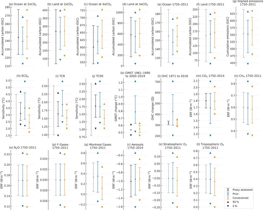
952                                   J. Tsutsui: MCE v1.2: a new simplified method for probabilistic climate projections

contribution to AR5, and the specific emulator plays a crucial   models were compared under the same set of constraints for
role in synthesizing the most comprehensive information on       model parameter perturbations (Nicholls et al., 2021).
climate projections available at the time.                          The MCE has been used in both phases, and the present
   However, the climate assessment of AR5 is regarded as         article provides details of the version used in Phase 2. The
indicative as it is based on a single probability distribution   MCE model consists of prediction equations for thermal re-
(Clarke et al., 2014). This is similar to the scenario assess-   sponse and carbon cycle. Although there are many emulators
ment of the 2018 IPCC Special Report on global warming           with different complexities, their core modules appear to be
of 1.5 ◦ C (SR15) (Rogelj et al., 2018), for which the same      based on a few pioneering works and are often shared be-
method as in AR5 was used for scenario classification but        tween different emulators. The thermal response of the MCE
noticeable differences in radiative forcing and temperature      is implemented as a pure impulse response model (IRM),
response were identified between the results of MAGICC           which is the most simplified form originated from the one
and of a different emulator, FaIR version 1.3 (Smith et al.,     presented in Hasselmann et al. (1993). The carbon cycle of
2018). FaIR incorporates recent updates of radiative forcing     the MCE is based on a part of the nonlinear impulse response
and shows greater non-CO2 anthropogenic forcing in histori-      model of the coupled carbon–climate system (NICCS; Hooss
cal and future periods than MAGICC (Forster et al., 2018). In    et al., 2001), which may be categorized to be of intermediate
contrast, current and projected warming is generally greater     complexity among RCMIP participants. One of them, ACC2
in MAGICC than in FaIR, implying greater climate sensitiv-       (Tanaka et al., 2007), also adopts the NICCS-based carbon
ity in the former.                                               cycle.
   With regard to climate sensitivity, the new CMIP Phase 6         Although complex formulations are generally more capa-
(CMIP6; Eyring et al., 2016) has been providing differ-          ble of emulation, they are not necessarily advantageous for
ent outcomes from CMIP5. Equilibrium climate sensitivity         emulating individual CMIP models and representing their
(ECS), a hypothetical value of global warming at equilibrium     uncertainty ranges. For thermal response, this has been con-
in response to a doubling of the atmospheric CO2 concentra-      firmed by the author’s previous studies (Tsutsui, 2017, 2020),
tion, is generally greater in CMIP6 models than in CMIP5         which have demonstrated that a simple IRM can accurately
models, mainly attributed to the models’ cloud processes         emulate a variety of CMIP models in terms of temperature
(Zelinka et al., 2020). Transient climate response (TCR), a      response to CO2 forcing and provide a basis of parameter
value of global warming at the time of CO2 doubling with an      sampling that covers model diversity. These findings also
idealized 1 %-per-year concentration increase, is also greater   imply that less complex emulators are suitable for knowl-
in CMIP6 than in CMIP5 models, but their relative differ-        edge transfer in a transparent way. From this perspective, key
ence is smaller than that of ECS (Meehl et al., 2020). This      considerations for emulator design are its subsidiary compo-
characteristic, reflecting the tendency of realized warming      nents, such as forcing parameterizations, treatment of nonlin-
fractions, specifically TCR-to-ECS ratios, is consistent with    ear processes involving some state-dependent response prop-
a theoretical relationship between climate feedback strength     erties, and parameter constraining for probabilistic projec-
and thermal response timescales (Tsutsui, 2020). However,        tions.
modeled historical warming generally appears greater in the         The remainder of this article is structured as follows. Sec-
CMIP5 models than in the CMIP6 models, supported by ex-          tion 2 describes model formulations and parameter sampling
tremely strong aerosol cooling as found in several CMIP6         methods. Section 3 presents the experimental application of
models (Flynn and Mauritsen, 2020), as well as generally         probabilistic climate projections. Section 4 discusses emula-
weaker greenhouse gas (GHG) forcing in CMIP6 models              tor performance and constraining model parameters. Finally,
(Smith and Forster, 2021).                                       Sect. 5 presents the study’s main conclusions.
   These confusing results require a more advanced and
transparent methodology to synthesize new insights into
forcing, response, and sensitivity, not only from climate
modeling but also from other lines of evidence. The Re-          2     Model description
duced Complexity Model Intercomparison Project (RCMIP;
Nicholls et al., 2020) is promising, providing the first com-    2.1    Impulse response models
prehensive model intercomparison of emulators. During
Phase 1 of this project, a new framework was established to      The MCE model is essentially built on impulse response
systematically evaluate multiple emulators from scenario ex-     functions for the fraction of the total CO2 emitted that re-
periments that mirror those in CMIP5 and CMIP6, and 15           mains in the atmosphere (termed the airborne fraction), the
emulators were compared in terms of their ability to approx-     decay of land carbon accumulated by the CO2 fertilization
imate each of the CMIP6 models, mainly in terms of global        effect, and temperature change to radiative forcing of CO2
mean temperature changes (Nicholls et al., 2020). Phase 2        and other forcing agents. Under the linear response assump-
then focused on probabilistic climate projections, and nine      tion with regard to input forcing F , an impulse response
                                                                 model (IRM) expresses the time change of a response vari-

Geosci. Model Dev., 15, 951–970, 2022                                              https://doi.org/10.5194/gmd-15-951-2022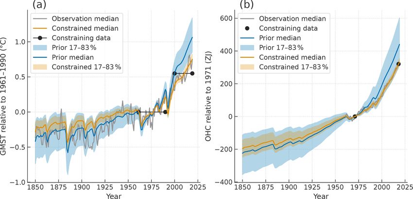
J. Tsutsui: MCE v1.2: a new simplified method for probabilistic climate projections                                                953

Figure 1. Schematic diagram of the box models equivalent to the MCE’s impulse response models. Bidirectional arrows represent heat and
carbon fluxes within each module of the thermal response and carbon cycle. The two modules are connected through CO2 forcing and climate
feedback mechanisms.

able x by a convolution integral:
          Zt
                                  t − t0

                      X
x (t) =        F t0      Ai exp −          dt 0 ,             (1)
                       i
                                    τ i
          0

where t is time, and the sum of exponentials is an impulse
response function with parameters Ai and τi denoting the
ith component of the response amplitude and time constant,
respectively. The time derivative of this equation is given by

dx (t) X                   xi (t)
       =        F (t) Ai −          ,                       (2)
  dt       i
                             τi

or an equivalent box model form that is converted into the            Figure 2. Response of the airborne fraction to an initial input of
original IRM through Laplace transform or eigenfunction ex-           100 Gt C without land CO2 uptake and climate feedback. The line
pansion. The time derivative implemented in the MCE uses              shows the case of reference amplitudes, and shading shows the
an IRM form for land carbon decay and temperature change              range of the 5th–95th percentiles of the Prior ensemble, which is
                                                                      described in Sect. 3.1.
and a box model form for the airborne fraction to address par-
titioning of excess carbon between the atmosphere and ocean
mixed layer. Figure 1 illustrates the MCE’s components in a
box model form representing heat or carbon reservoirs. Since
each component is formulated on its own impulse response              to a specific three-dimensional ocean carbon cycle model in
functions, the boxes are separately defined between the ther-         Hooss et al. (2001). The corresponding amplitudes assume
mal response and carbon cycle modules.                                perturbations at reference values of 0.24, 0.21, 0.25, and 0.1,
    The IRM for the airborne fraction defines five components,        respectively, with a reference long-term airborne fraction of
one of which has an infinity time constant, paired with an am-        0.20. These reference values and perturbation ranges are set
plitude corresponding to an asymptotic long-term fraction. In         empirically so that resulting carbon budgets – cumulative
the current configuration, the remaining four time constants          land and ocean CO2 uptake – agree with those of historical
are fixed at 236.5, 59.52, 12.17, and 1.271 years, adjusted           observations and CMIP experiments.

https://doi.org/10.5194/gmd-15-951-2022                                                     Geosci. Model Dev., 15, 951–970, 2022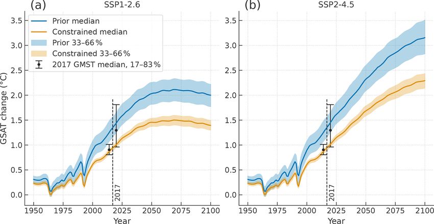
954                                     J. Tsutsui: MCE v1.2: a new simplified method for probabilistic climate projections

   As described below, IRM parameters are converted into a           tically optimal choice (Cummins et al., 2020). Separating the
set of parameters for an equivalent box model dealing with           intermediate time constant is also beneficial for representing
carbon exchange between four layers. In this conversion, the         a pattern effect – warming response affected on a decadal or
response of the shortest timescale component is interpreted          multi-decadal timescale by the changing pattern of surface
as equilibration between the atmosphere and ocean mixed              warming (e.g., Andrews et al., 2015). The response ampli-
layer, which are combined into a composite layer in the box          tude is rewritten by Ãi /(λτi ), where Ãi is normalized so that
model, as shown in the ocean carbon cycle in Fig. 1. Fig-            the component sum is unity, and λ is the climate feedback pa-
ure 2 shows response to an idealized instantaneous input of          rameter (W m−2 ◦ C−1 ), defined as the derivative of the out-
100 Gt C without land carbon uptake and climate feedback.            going thermal flux with respect to temperature change. These
In this case, the airborne fraction decreases from 0.9 to a          IRM parameters can be adjusted to emulate individual CMIP
long-term equilibrium of about 0.2 at a gradually decreasing         models with sufficient accuracy, as demonstrated in Tsutsui
rate. The asymptotic long-term airborne fraction is slightly         (2020), which serves a basis to build a perturbed parameter
greater than an assumed value, depending on the size of pulse        ensemble.
input, due to the buffering mechanism of seawater.
   The IRM for land carbon defines four carbon pools, rep-           2.2   Carbon uptake over ocean
resenting ground vegetation, wood, detritus, and soil organic
carbon, with distinct overturning times (τi ). The forcing term      The box model converted from the IRM for the airborne frac-
(F ) is net primary production (NPP) enhanced by the effect          tion is as follows:
of CO2 fertilization, generally expressed by βL N0 , where βL        dc0        η1      η1
                                                                          = − cs + c1 + e − f,                               (3)
is a fertilization factor that depends on the atmospheric CO2         dt        hs      h1
concentration, and N0 is base annual NPP (Gt C yr−1 ). The           dc1      η1      η1 + η2     η2
response amplitude (Ai ) is rewritten as Ãbi τi , where Ãbi de-         = cs −              c1 + c2 ,                      (4)
                                                                      dt      hs         h1       h2
notes a decay flux after an initial carbon input. Based on Joos      dc2      η2      η2 + η3     η3
et al. (1996), the IRM parameters of the four carbon pools                = c1 −              c2 + c3 ,                      (5)
                                                                      dt      h1         h2       h3
are set to 2.9, 20, 2.2, and 100 years for τi and 0.70211,
                                                                     dc3      η3      η3
0.013414, −0.71846, and 0.0029323 yr−1 for Ãbi , respec-                 = c2 − c3 ,                                        (6)
tively. Figure 3 illustrates response to unit forcing in this con-    dt      h2      h3
figuration.                                                          where ck is the amount of excess carbon in layer k, hk is the
   In addition, the MCE deals with temperature dependency            layer depth, ηk is the exchange coefficient between layer k−1
for the time constants of wood and soil organic carbon, in-          and layer k, e is anthropogenic emissions, and f is natural
dicating the tendency for warming to accelerate the decom-           uptake over land. The parameters hk and ηk are set through
position of organic matter. This is one of the climate–carbon        numerical optimization for the box model to be equivalent to
cycle feedback processes and is implemented with an adjust-          the IRM form. The top layer, indexed with 0, is the composite
ment coefficient varied along a logistic curve with respect          atmosphere–ocean mixed layer, and the three subsurface lay-
to surface warming, as illustrated in Fig. 4. This scheme            ers are indexed with 1, 2, and 3 in the order of ocean depth.
has a parameter to control the asymptotic minimum value              The amount of excess carbon in the top layer (c0 ) is parti-
of the coefficient. The figure shows three curves with differ-       tioned into atmospheric and ocean components, denoted by
ent control parameters, corresponding to the 5th, 50th, and          ca and cs , subject to chemical equilibrium at the ocean sur-
95th percentiles of the Prior ensemble, which is described           face. The carbon exchange between the top layer and the first
in Sect. 3.1, adjusted to be consistent with the variation of        subsurface is expressed in terms of cs .
CMIP Earth system models (ESMs). InP        the IRM form, land          For a given time series of CO2 emissions (emission-
accumulated carbon is proportional to Ãbi τi2 , expressing          driven) or atmospheric CO2 concentrations (concentration-
                                            i                        driven), time integration is performed. In the latter case, c0
the remaining carbon at an equilibrium state under unit con-
                                                                     and its partition within the composite layer are diagnostically
tinuous input, and the decrease in the time constants affects
                                                                     determined, and the top layer equation is dropped.
accumulated carbon quadratically.
                                                                        The partition of c0 is solved through numerical compu-
   The IRM of the temperature change defines three compo-
                                                                     tation with regard to hydrogen ion concentration associ-
nents with typical time constants of approximately 1, 10, and
                                                                     ated with changes in dissolved inorganic carbon concen-
> 100 years. Although the temperature response is usually
                                                                     tration (DIC) under the assumption of constant alkalinity
well represented by two separated time constants of approx-
                                                                     (Alk). DIC, defined as the sum of [CO2 ], [HCO−       3 ], and
imately 4 and > 100 years (e.g., Held et al., 2010; Geoffroy              2−
et al., 2013), dividing fast response is advantageous when           [CO3 ], where [x] denotes the concentration of a substance
considering instantaneous forcing changes, such as volcanic          x (mol L−1 ), is expressed as
                                                                                                    !
eruptions (Gupta and Marshall, 2018) and geoengineering                              K1      K1 K2
mitigation, and using three time constants appears to be prac-       DIC = 1 +  +  + + 2 [CO2 ] ,                              (7)
                                                                                     H       [H ]

Geosci. Model Dev., 15, 951–970, 2022                                                  https://doi.org/10.5194/gmd-15-951-2022
J. Tsutsui: MCE v1.2: a new simplified method for probabilistic climate projections                                               955

Figure 3. Response of land carbon to instantaneous unit input (a) and accompanying flux from carbon pools (b).

                                                                       borate and water, defined as [H+ ][B(OH)−    4 ]/[B(OH)3 ] and
                                                                       [H+ ][OH− ].
                                                                          The values of Alk, BT , and the equilibrium constants
                                                                       of K0 , K1 , K2 , Kb , and Kw are set based on Dickson et
                                                                       al. (2007). The equilibrium constants depend on water tem-
                                                                       perature, and carbon uptake decreases with temperature, rep-
                                                                       resenting a climate–carbon cycle feedback process. This tem-
                                                                       perature dependency is implemented as a linear regression
                                                                       for empirical expressions, as shown in Fig. 5.
                                                                          The amount of excess carbon that can be accumulated
                                                                       in the ocean is proportional to a change in DIC from its
                                                                       preindustrial value. This carbon uptake potential and its tem-
                                                                       perature dependency are illustrated in Fig. 6. CO2 -induced
                                                                       global warming increases the airborne fraction in two ways
                                                                       – through the buffering mechanism of seawater and through
Figure 4. Adjustment coefficient as a function of surface tempera-     temperature dependency of chemical equilibrium. The for-
ture change to multiply the time constants for the decay of wood and   mer is shown as a decreasing change rate of the DIC with
soil organic matter. The three curves are functions corresponding to   regard to atmospheric CO2 concentration (Fig. 6a), while the
the 5th, 50th, and 95th percentiles of the Prior ensemble, which is    latter is shown as a reduction in rates of carbon uptake po-
described in Sect. 3.1, with different asymptotic minimum values,      tential with temperature, which also depends on the concen-
as described in the legend. The temperature at which a curve has the
                                                                       tration (Fig. 6b). The reduction rate is approximately propor-
maximum gradient is fixed at 3.5 ◦ C.
                                                                       tional to the warming level, typically about 4 % per 1 ◦ C at
                                                                       doubling CO2 .
where K1 and K2 are equilibrium constants for bicarbon-
ate and carbonate, defined as K1 = [H+ ][HCO−   3 ]/[CO2 ] and         2.3   CO2 fertilization
K2 = [H+ ][CO2− 3 ]/[HCO  −
                          3 ]. [CO 2 ], defined as the sum of
[CO2 (aq)] and [H2 CO3 (aq)], is related to the partial pres-          The land carbon uptake term f in Eq. (3) is calculated from
sure of CO2 (pCO2 ) with equilibrium constant K0 , as in               Eq. (2), rewritten as
K0 = [CO2 ]/pCO2 . Alkalinity, here considering borate ions
as well as bicarbonate and carbonate ions, is represented as                     X
                                                                                                       cbi
                                                                       f (t) =     βL (t) N0 Ãbi τi −       ,                    (9)
       K1 H+ + 2K1 K2                                                                                  τi

                                        Kb BT                                    i
Alk =                      [CO2 ] +
              [H+ ]2

                                     Kb + H+
        Kw                                                             where cbi is the ith component of accumulated carbon by
     +  +  − H+ ,

                                                            (8)        CO2 fertilization. The base NPP (N0 ) is set to 60 Gt C yr−1
        H
                                                                       and the fertilization factor (βL ) is formulated with a sigmoid
where BT is total borate concentration [B(OH)3 ] +                     curve with regard to CO2 concentration C(t), as described in
[B(OH)−
      4 ], and Kb and Kw are equilibrium constants for                 Meinshausen et al. (2011). This implementation is connected

https://doi.org/10.5194/gmd-15-951-2022                                                      Geosci. Model Dev., 15, 951–970, 2022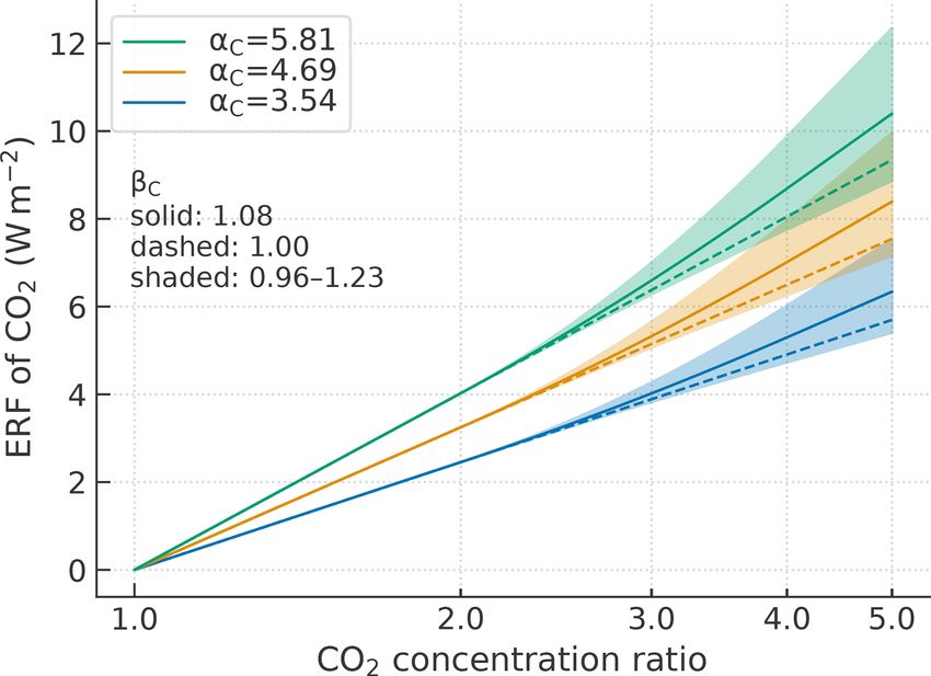
956                                      J. Tsutsui: MCE v1.2: a new simplified method for probabilistic climate projections

Figure 5. Temperature-dependent equilibrium constants of K0 , K1 , K2 , Kb , and Kw (a–e) in the MCE model (solid lines), which approx-
imate empirical expressions in Dickson et al. (2007) (D07, dotted lines). Values at a reference seawater temperature of 13.5 ◦ C (dots) are
assigned to those in the MCE’s preindustrial state.

Figure 6. DIC in the ocean mixed layer as a function of atmospheric CO2 concentration (a) and changes in ocean carbon uptake potential,
measured by the increase in DIC from preindustrial levels, due to 1 and 2 ◦ C warming (b). The preindustrial CO2 concentration is assumed
to be 284.317 ppm, and preindustrial DIC is about 2.17 mmol L−1 .

to a conventional logarithmic formula,                                  2.4   Effective radiative forcing

                  C (t)                                                 The forcing term in the IRM for temperature change is as-
βL = 1 + β̂L ln           ,                                   (10)
                  C (0)                                                 sumed to be effective radiative forcing (ERF), defined as top-
                                                                        of-atmosphere (TOA) radiative imbalance due to a change in
such that the sigmoid and logarithmic curves are equal in               a forcing agent through rapid adjustments in the stratosphere
terms of an increase ratio at 680 ppm relative to 340 ppm, and          and troposphere prior to a response in surface temperature
the latter factor β̂L is used as a control parameter. Figure 7          (Myhre et al., 2013; Sherwood et al., 2015). Forcing, defined
illustrates three curves with different control parameters in           as such, serves as a good predictor of surface temperature
the MCE model.                                                          change.

Geosci. Model Dev., 15, 951–970, 2022                                                      https://doi.org/10.5194/gmd-15-951-2022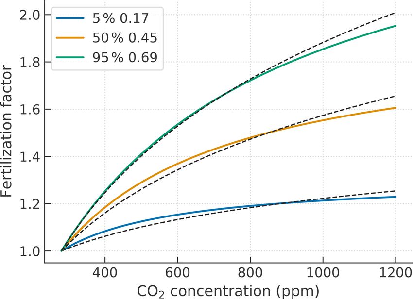
J. Tsutsui: MCE v1.2: a new simplified method for probabilistic climate projections                                                     957

Figure 7. CO2 fertilization factor as a function of atmospheric CO2     Figure 8. Effective radiative forcing (ERF) of CO2 as a function of
concentration with different control parameters (β̂L ) of 0.17, 0.45,   the ratio of CO2 concentrations to a preindustrial level. The scaling
and 0.69, corresponding to the 5th, 50th, and 95th percentiles of       parameter αC is set to three different values, corresponding to the
the Prior ensemble described in Sect. 3.1. The colored lines show       5th, 50th, and 95th percentiles of the Prior ensemble described in
sigmoid curves used in the MCE model, and the black dashed lines        Sect. 3.1. For each αC value, the amplification factor βC is varied
show reference logarithmic curves.                                      between the 5th and 95th percentiles (shaded area) and is set to two
                                                                        specific values of the 50th percentile (solid line) and unity (dashed
                                                                        line, no amplification).
   CO2 forcing is evaluated with the following quadratic for-
mula in terms of the logarithm of CO2 concentration:
                     h                 i
FC (x) = (βC − 1) F̂C (x) − 2FC (2)                                        The forcing of CH4 and N2 O is evaluated with the expres-
          "             #                                               sions given in Etminan et al. (2016). The forcing of halo-
            2F̂C (x)                                                    genated gases is simply calculated as changes in concentra-
        ·            − 1 + βC F̂C (x) ,                 (11)            tion from preindustrial levels multiplied by radiative efficien-
             FC (2)
                                                                      cies assessed in the latest IPCC report (at the time of this
                   CO2 (t)                                              paper preparation AR5; Myhre et al., 2013).
F̂C (x) = αC ln              ,                          (12)
                   CO2 (0)                                                 The current MCE model does not support non-CO2 gas
                                                                        cycles and ERF schemes for other forcing agents, such as
where x is the ratio of CO2 concentrations to a preindus-               aerosols, tropospheric and stratospheric ozone, solar radia-
trial level, αC is a scaling parameter (W m−2 ), and βC is              tion, and volcanic eruptions. Experiments considering non-
an amplification factor defined as FC (4) = βC × F̂C (4). This          CO2 forcing require prescribed concentrations for long-lived
scheme was presented in Tsutsui (2017) to emulate the                   GHGs and prescribed ERF for others.
CMIP’s core CO2 increase experiments for instantaneous
quadrupling and 1 %-per-year increase, referred to as abrupt-
4xCO2 and 1pctCO2, respectively. Thus, the scheme is valid              2.5   Parameter sampling
in the range of 1 ≤ x ≤ 4. The two control parameters are
diagnosed consistently with IRM parameters for individual               Probabilistic runs use an ensemble of perturbed model pa-
CMIP models (Tsutsui, 2020). The current diagnosing pro-                rameters designed to encompass the variation of multiple
cedure solves numerical optimization to approximate the first           CMIP models with additional constraints with regard to as-
150-year and 140-year time series from abrupt-4xCO2 and                 sessed ranges of key climate indicators. In general, a series of
1pctCO2 experiments, respectively, in terms of TOA energy               candidate values of an uncertain parameter is generated from
imbalance and the surface air temperature anomaly, respec-              its statistical model and, if necessary, sampled from the series
tively. The quadratic term is activated when the concentra-             with an acceptance algorithm for given constraints. The latter
tion exceeds 2 times (x > 2), and βC is set to unity in the             process is Bayesian updating from a prior probability distri-
range x ≤ 2 so that FC is equivalent to F̂C . The forcing am-           bution to a posterior and uses a Metropolis–Hastings (MH)
plification is expected to be valid in the range x ≤ 4 and the          independence sampler here. As mentioned above, uncertain
quadratic term is dropped beyond a level of 4 times. Figure 8           parameters include IRM amplitudes for the airborne fraction,
illustrates example outputs of the CO2 forcing scheme in a              control parameters for land carbon decay timescales and CO2
range of 5th–95th percentiles of the Prior ensemble for con-            fertilization, IRM parameters for temperature change, and
trol parameters.                                                        control parameters for the CO2 forcing scheme.

https://doi.org/10.5194/gmd-15-951-2022                                                       Geosci. Model Dev., 15, 951–970, 2022
958 J. Tsutsui: MCE v1.2: a new simplified method for probabilistic climate projections
In a Bayesian framework, some difficulties arise from set- The eight parameters to be fed into PC analysis can include
ting appropriate prior distributions and dealing with large- some derived parameters from the following expressions:
dimension likelihood functions. Although the latter can be
avoided by using the Markov chain Monte Carlo (MCMC) Ãi X
approach, its implementation, typically based on the MH Ai = , Ãi = 1, (13)
λτi i
algorithm, is not necessarily straightforward in exploring a
αC ln (2)
large-dimension parameter space with the detailed balance ECS = , (14)
that underlies MCMC. One of the relevant issues is sampling λ
efficiency. Goodwin and Cael (2021), for example, generated αC βC ln (2)
ECSG = , (15)
a prior by varying a set of ∼ 25 model parameters indepen- (λ )
dently with a very large size of ∼ 109 and constrained it by an X τi
t70
acceptance algorithm with an observation-based likelihood TCR = ECS 1 − Ãi 1 − exp − , (16)
i
t70 τi
function. Although the prior ensemble size can be reduced
by improving the acceptance algorithm (Goodwin, 2021), it where ECS is defined using a diagnosed forcing of CO2 dou-
appears to need ∼ 107 to get a posterior for typical applica- bling, while ECSG uses CO2 quadrupling with a factor of 0.5
tion, such as climate sensitivity estimation and probabilistic as in Gregory et al. (2004). Equation (16) is derived from
climate projections. time integration of Eq. (1) to the 70th year (t70 ) along a 1 %-
The current MCE approach is one way to deal with the per-year increasing path that defines TCR. One possible set
above difficulties. Setting a prior with statistical models rep- consists of TCR, Ã0 /Ã2 , Ã1 /Ã2 , τ0 , τ1 , τ2 , αC , and βC , ap-
resenting a CMIP multi-model ensemble allows the use of an plied with logarithmic transformation, except for αC . This set
efficient MH independence sampler, with the size of a prior was adopted in the experiments described below. The loga-
series for typical applications expected to be ∼ 104 or at most rithmic transformation is intended to allow fair normality of
∼ 105 . It is also convenient that this sampler is free from PC scores as a basis for fitting a multivariate normal distri-
adjustment, unlike random-walk-based MCMC implementa- bution and to make generated candidates positive.
tion that requires step-size adjustment. One thing to note is Probabilistic runs can also use different scaling factors to
that the independence sampler is suitable when the proposed adjust individual non-CO2 ERF time series. This is a simple
prior series encompasses the target posterior series, and the implementation to deal with non-CO2 forcing uncertainties,
acceptance rate of sampling is high to some extent. However, typically assessed as a range at a reference time point. The
this requirement is not met for the case presented below. This scaling factor is perturbed with a suitable statistical model
problem is addressed in the implementation of the MH algo- fitted to the range.
rithm in Sect. 3 and further discussed in Sect. 4. All uncertain parameters and ERF scaling parameters are
The carbon cycle parameters are individually generated not necessarily independent. The current sampling procedure
from a uniform distribution with a given mean and pertur- incorporates covariance between the eight parameters rele-
bation range. The means and ranges are determined on a trial vant to temperature change in response to CO2 forcing. How-
basis so that ranges of carbon budgets in historical and sce- ever, the procedure assumes no other correlations, implying
nario experiments are consistent with those from multiple that uncertainties of the CO2 -induced temperature response
CMIP ESMs. Since the sum of IRM amplitudes for the air- are independent from those of the carbon cycle and non-CO2
borne fraction is unity, their perturbed values are normalized forcing.
as such, subject to a modified distribution with more samples
about the mean resulting from the operation.
The temperature response and CO2 forcing parameters are 3 Application examples
synthetically generated from a multivariate normal distribu-
tion reflecting the variation of multiple CMIP AOGCMs. The 3.1 Scenario experiments
IRM for temperature change has three pairs of time constant
(τi ) and dimensional amplitude (Ai ), and the CO2 forcing To demonstrate a typical application of the MCE model,
scheme has two control parameters (αC and βC ). A total of a number of scenario experiments that mirror those of
eight parameters have been diagnosed for each of the multi- CMIP6 were conducted, including idealized abrupt-4xCO2
ple CMIP models, revealing characteristic covariance struc- and 1pctCO2, as well as historical–future scenarios based
tures, such as a noticeable negative correlation between feed- on the Shared Socioeconomic Pathways (SSPs; Riahi et al.,
back strength (1/λ) and a realized warming fraction (typi- 2017). In the latter experiments, the model was initialized for
cally TCR-to-ECS ratio), as well as a weakly negative corre- the year 1850 and driven with GHG concentrations and other
lation between the forcing scale (αC ) and feedback strength prescribed ERF, both provided from the RCMIP (Nicholls et
(Tsutsui, 2020). The multivariate normal distribution is built al., 2020).
on principal components (PCs) of these diagnosed parame- For each scenario, two sets of 600-member ensemble runs
ters, as described in Tsutsui (2017). were conducted; one was perturbed to be consistent with a
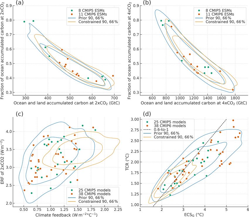
Geosci. Model Dev., 15, 951–970, 2022 https://doi.org/10.5194/gmd-15-951-2022J. Tsutsui: MCE v1.2: a new simplified method for probabilistic climate projections 959 CMIP multi-model ensemble and the other was further con- Besides CO2 forcing, the RCMIP constraints include strained according to the RCMIP Phase 2 protocol (Nicholls the ranges of non-CO2 forcing over a historical period et al., 2021), here labeled Prior and Constrained, respectively. for CH4 , N2 O, halocarbons (aggregated into “Montreal Prior refers to 25 CMIP5 and 38 CMIP6 AOGCMs for the gases” – CFCs, HCFCs, halons – and other “F gases” PC analysis input and to 8 CMIP5 and 11 CMIP6 ESMs – HFCs, PFCs, SF6 ), aerosols (aggregated), tropospheric diagnosed in Arora et al. (2020) for simulated carbon bud- ozone, stratospheric ozone, stratospheric water vapor from gets in the 1pctCO2 experiment. Diagnosed forcing and re- CH4 , and albedo change due to land use and black carbon sponse parameters of the multiple AOGCMs are presented in aerosols on snow and ice. Ranges are based on AR5 (Myhre the MCE’s code repository. et al., 2013), except for those for CH4 and aerosols, which The uncertain carbon cycle parameters for Prior were gen- consider recent updates (Etminan et al., 2016; Smith et al., erated from the abovementioned statistical models, as shown 2020). To incorporate these uncertainty ranges in historical- in Figs. 1, 3, and 6, and were processed by the MH sam- future scenarios, the scaling factors to adjust individual non- pler to constrain accumulated land carbon at doubling CO2 CO2 ERF time series were perturbed using normal or skewed along the 1 %-per-year pathway. In this case, 1pctCO2 sce- normal distributions fitted to the prescribed ranges. nario runs with a set of proposed parameters were conducted The RCMIP constraints are provided as likely ranges and to obtain data fed into the sampler. This single constraint was optionally very likely ranges, corresponding to 17 %–83 % selected as it works inclusively for other relevant constraints and 5 %–95 % according to the IPCC’s likelihood terms. through a trade-off relationship between ocean and land in These ranges were applied to generate uncertain parameter terms of accumulated carbon. proposals and to build the MH sampler requiring probability RCMIP Phase 2 defines a number of constraints for cli- densities for a target distribution. mate indicators, including ERF levels, carbon budgets, re- Although a number of indicators were prepared for the cent warming trends, and climate sensitivity metrics of ECS, RCMIP constraints, a very limited number of those were TCR, and transient climate response to cumulative CO2 used here, partly because the prior was designed to match emissions (TCRE). Here, TCRE is defined as the ratio of some of them like the forcing constraints and partly because the TCR to implied cumulative CO2 emissions at the time the proxy assessment ranges are not necessarily consistent of CO2 doubling along the same 1 %-per-year trajectory as with each other. The sequence of the MH sampler for the that for TCR. These constraints use literature-based assessed above three items, which relaxes the detailed balance re- ranges, referred to as a “proxy assessment”, to distinguish quired for MCMC, was established to deal with those con- these from the formal IPCC assessment. The Constrained un- straints and needs to be improved using fully consistent as- certain parameters were sampled from those of Prior through sessment ranges. a sequence of the MH sampler with a subset of RCMIP Other details of the constraining procedures and experi- constraints, as follows: (1) CO2 ERF in 2014 relative to mental specifications are provided in the MCE’s code repos- 1750 evaluated in Smith et al. (2020), (2) TCR estimated itory (see “Code and data availability” at the end). in Tokarska et al. (2020, Table S3, both constrained), and (3) GMST in the period 1961–1990 relative to the period 3.2 Results: climate indicators 2000–2019 from the HadCRUT.4.6.0.0 dataset (Morice et al., 2012) and ocean heat content (OHC) in 2018 relative to 1971 Figure 9 illustrates relationships between key indicators as- from the dataset of von Schuckmann et al. (2020). In this sociated with the carbon budget and climate sensitivity of the case, in addition to 1pctCO2 runs, historical scenario runs two ensembles in comparison with the CMIP models. The with a set of proposed parameters were conducted to obtain carbon budget is measured by the amount of accumulated data fed into the sampler. carbon and its allocation to ocean and land reservoirs. Here, The IRM for temperature change is transformed into a total accumulation and the ocean allocation ratio at doubling three-layer heat exchange model in physical space (Fig. 1). and quadrupling CO2 levels are used as key indicators. The The top layer is representative of fast-responding Earth sys- CMIP ESMs indicate a clear negative correlation between the tem components – the atmosphere and Earth’s surface includ- two quantities (Fig. 9a and b), reflecting much greater uncer- ing a part of the ocean mixed layer. However, when diagnos- tainties relating to land carbon. This feature is well repre- ing the CO2 forcing and response parameters, the top layer sented by the MCE parameter ensembles. Although there are temperature was treated as global mean surface air tempera- some model differences between CMIP5 and CMIP6 eras, ture (GSAT) in practice. As in HadCRUT GMST was defined such as a reduced model spread in the latter associated with as a surface air–ocean blended temperature change; here, a nitrogen cycle implementation (Arora et al., 2020), the MCE factor of 1.04 was used to convert observed GMST change ensembles currently do not distinguish between the two. The into the MCE’s GSAT change. Likewise, as the MCE’s three carbon indicators of the Constrained ensemble do not differ layers cannot be allocated to specific climate system compo- significantly from those of Prior but are distributed toward nents, a factor of 1.08 was used to convert observed OHC higher total accumulations, which is attributed to warming change into the MCE’s total heat content change. differences that affect carbon cycle–climate feedbacks. https://doi.org/10.5194/gmd-15-951-2022 Geosci. Model Dev., 15, 951–970, 2022
960                                      J. Tsutsui: MCE v1.2: a new simplified method for probabilistic climate projections

Figure 9. Relationships between key indicators associated with carbon budget and climate sensitivity in comparison with CMIP models.
Contours indicate kernel density levels at which the circles cover 90 % and 66 % of members. The legend indicates the number of the CMIP
models. (a) The fraction of ocean accumulated carbon as well as ocean and land totals in the 70th year of 1pctCO2. (b) Same as panel (a),
but in the 140th year. (c) Effective radiative forcing (ERF) of CO2 doubling and climate feedback parameter. (d) Transient climate response
(TCR) and equilibrium climate sensitivity diagnosed from abrupt-4xCO2 (ECSG ). The dashed line is located where the ratio of TCR to
ECSG is 0.6 as a reference.

   In contrast, climate sensitivity differences are most promi-         ity is more evident in ECSG than in TCR. The inherent rela-
nent and well characterized with key indicators’ distribu-              tionship between feedback strength and response timescales
tions on two-dimensional domains: the ERF of CO2 dou-                   is responsible for the tendency, together with the forcing am-
bling derived from αC vs. the climate feedback parameter                plification effect represented by βC . The PC-analysis-based
(λ) (Fig. 9c) and TCR vs. ECSG (Fig. 9d). While the Prior               statistical model captures such covariance structure effec-
distributions cover the CMIP AOGCMs effectively, the Con-               tively.
strained distributions are confined to lower sensitivity val-              Figure 10 illustrates historical GMST and OHC of the
ues – greater λ and smaller TCR and ECSG , which is at-                 MCE’s two ensembles in comparison with their observa-
tributed to the observed GMST and OHC constraints. The                  tions, from which constraining data are considered for recent
Prior distribution of the CO2 forcing agrees well with the              warming trends. In the figure, the time series are adjusted
CMIP distribution, which shows a weakly positive correla-               relative to the reference period 1961–1990 for GMST and
tion with the climate feedback parameter. In contrast, the              the reference year 1971 for OHC. While the Prior series are
Constrained forcing levels are confined to an upper half of             well above the observed warming during the target period
the CMIP AOGCMs, which is attributed to the historical CO2              2000–2019 for GMST and during the target year 2018 for
forcing constraint, and the forcing–feedback correlation be-            OHC, the Constrained series agree well with recent trends.
comes weak. Transient sensitivity is not necessarily propor-            The observation-based constraining results in lower climate
tional to equilibrium sensitivity, and greater CMIP6 sensitiv-          sensitivity in the latter ensemble. However, considerable un-

Geosci. Model Dev., 15, 951–970, 2022                                                      https://doi.org/10.5194/gmd-15-951-2022
J. Tsutsui: MCE v1.2: a new simplified method for probabilistic climate projections                                                   961

Figure 10. (a) Historical global mean surface temperature (GMST) relative to 1961–1990 and (b) historical ocean heat content (OHC) relative
to 1971 in the period 1850–2019 compared with observation data from HadCRUT4.6.0.0 for GMST and von Schuckmann et al. (2020) for
OHC. The black dots indicate the levels in two different periods or years used for the observation constraints.

certainties remain with regard to longer trends and unforced            wider and higher than assessed ranges but comparable Con-
climate variability. In an earlier period, observed GMST was            strained ranges. The consistency of sensitivity indicators, in-
rather close to Prior, and the Constrained trend appears to be          cluding TCRE (Fig. 12h–j), is complex because the proxy
underestimated. The OHC trend cannot be validated owing                 assessment ranges (black error bars) themselves are not nec-
to its limited observation period. Assessment of forced re-             essarily consistent with each other, as discussed in the next
sponse in the historical period, which is currently not avail-          section, and narrowed from the AR5-assessed ranges (grey
able, would allow more reliable parameter sampling. Some                error bars). Overall, consistency is better for Prior ranges, al-
variation in the historical forcing time series, in particular for      though Constrained ranges, which are considerably narrowed
aerosols (Smith et al., 2021), would also be worth exploring.           and lowered, are still within the AR5-assessed ranges. The
   The greater warming in Prior is not only due to its greater          ranges of the carbon cycle indicators (Fig. 12a–g), includ-
climate sensitivity, but also partly due to non-CO2 forcing             ing accumulated carbon and implied cumulative emissions
differences, as shown in Fig. 11. The scaling factors of the            in the historical period 1750–2011, are not significantly dif-
non-CO2 forcing agents are independently perturbed in the               ferent between the two ensembles and broadly agree with as-
Prior ensemble and probabilistically selected through the se-           sessed ranges. Ensemble runs for the extended historical pe-
ries of the MH sampler. Although the sampling process does              riod starting from 1750 were conducted for calibration. The
not directly refer to forcing levels of non-CO2 agents, it can          ranges of the ERF indicators (Fig. 12m–t) are consistent with
modify their distributions to be consistent with other con-             assessed ranges, except for Prior CO2 and Constrained Mon-
straints. This modification is found for non-CO2 GHGs and               treal gases, as mentioned above. Other minor changes from
ozone time series (Fig. 11b), and the most dominant contri-             Prior to Constrained include a reduced range for aerosols and
bution is of Montreal gases (not shown). The ERF of Mon-                lowered ranges for stratospheric and tropospheric ozone.
treal gases rapidly increases from the 1960s and levels off
from the 1990s, and the sampling results imply that this ten-           3.3   Results: projected warming
dency is not consistent with the recent warming trend. To-
tal ERF fluctuates with changes in solar irradiance and vol-            Figure 13 illustrates temperature response in two SSP sce-
canic eruptions, for which the RCMIP’s prescribed forcing               narios, SSP1–2.6 and SSP2–4.5, wherein warming is mea-
was used without their efficacy uncertainties.                          sured by an increase in global mean surface air temperature
   Figure 12 displays the ranges of climate indicators from             (GSAT) relative to 1850–1900, and the period up to 2100 is
the two ensembles associated with the carbon cycle, climate             presented. In the scenario labeled SSPn-x.x, “n” (1–5 num-
sensitivity, warming trends, and historical ERF changes in              bers) identifies different socioeconomic development path-
comparison with their proxy assessment ranges. The consis-              ways, and “x.x” expresses a nominal forcing level (W m−2 )
tency between modeled and proxy ranges can be most dis-                 at the end of the 21st century. The shaded areas indicate
tinctively shown for warming trends by GMST and OHC                     33 %–66 % ranges. The upper bound corresponds to the level
changes (Fig. 12k and l), with Prior ranges substantially               to which warming is likely (66 %–100 %) to be limited at the

https://doi.org/10.5194/gmd-15-951-2022                                                       Geosci. Model Dev., 15, 951–970, 2022
962                                   J. Tsutsui: MCE v1.2: a new simplified method for probabilistic climate projections

Figure 11. Historical effective radiative forcing (ERF) in the period 1850–2019 for total ERF (a) and aggregated components (b). The
ensembles’ medians are shown by lines, and the 5 %–95 % range of the Constrained ensemble is shown for the total by shading.

time, while the lower bound corresponds to the level which          ing is defined as an air–ocean blended temperature and is
warming is likely to exceed. These thresholds are shown in          thereby somewhat underestimated for the GSAT definition
Table 1 for peak and end-of-century (end-21C) warming for           (Schurer et al., 2018) with which modeled future warming
eight SSP scenarios, wherein the end-21C period is set to           is evaluated. In any case, the AR5 assessment is effectively
2081–2100 in accordance with the AR5.                               constrained by observed warming, which may be responsi-
   Regarding consistency with target warming levels, such           ble for its better agreement with the Constrained ensemble.
as 2 ◦ C above preindustrial levels, the Constrained ensem-         Figure 13 indicates medians and likely (17 %–83 %) ranges
ble agrees relatively well with the AR5 assessment (Collins         of temperature changes in 2017 by the GMST (air–ocean
et al., 2013) for each of the comparable Representative Con-        blended) definition: 1.30 [0.96–1.81] ◦ C in Prior and 0.90
centration Pathways (RCPs; van Vuuren et al., 2011) such as         [0.80–1.01] ◦ C in Constrained. The latter warming levels are
RCP2.6 with SSP1–2.6. For example, AR5 states that end-             also closer to the SR15 assessment of 1.0 [0.8–1.2] ◦ C for
21C temperature change above 2 ◦ C is unlikely (0 %–33 %)           human-induced warming (Allen et al., 2018), despite some
under RCP2.6, which implies that temperature is likely lim-         bias towards the lower end of the assessed range.
ited to 2 ◦ C. This assessment is consistent with the SSP1–2.6
result from Constrained (likely limited to 1.51 ◦ C) but not
from Prior (likely limited to 2.27 ◦ C). Some threshold tem-
peratures in Constrained are not consistent with AR5 such           4     Discussion
that the temperature in SSP2–4.5 likely exceeds 2.06 ◦ C,
while in AR5 it is more likely than not (> 50 %–100 %) to           4.1    Performance as an emulator
exceed 2 ◦ C in RCP4.5. There is a similar difference in the
possibility of limiting to 4 ◦ C in SSP5–8.5 and RCP8.5. AR5        It has already been confirmed that the MCE reproduces many
assessed these cases with medium confidence rather than             different CMIP models effectively in terms of thermal re-
high confidence, implying that the reduced likely ranges (as        sponse to idealized CO2 forcing changes, as demonstrated in
in Constrained) can update the AR5 assessment more au-              Nicholls et al. (2020). The forcing and response parameters
thentically. However, at present, the Constrained ensemble          are adjusted to emulate two of the CMIP’s basic experiments
does not incorporate possible uncertainties, as discussed in        for step-shaped (abrupt-4xCO2) and ramp-shaped (1pctCO2)
the next section. It should also be noted that SSP forcing is       forcing increases. The forcing scheme uses different func-
not exactly the same as corresponding RCP forcing, leading          tions depending on concentration levels: a quadratic expres-
to noticeable temperature differences between the compara-          sion in terms of logarithmic concentrations in the range from
ble scenarios (Nicholls et al., 2020).                              2 to 4 times the base level, smoothly connecting to linear ex-
   There are also some issues with handling of historical           pressions outside this range. This flexibility suits the CMIP
warming. The AR5 refers to a specific level of 0.61 ◦ C from        models’ tendency to deviate from logarithmic concentration
HadCRUT data for the period 1986–2005, which is added to            proportions at higher concentrations, leading to better emu-
the CMIP5 projected warming. However, HadCRUT warm-                 lation not only for responses to quadrupling increases com-

Geosci. Model Dev., 15, 951–970, 2022                                                  https://doi.org/10.5194/gmd-15-951-2022
J. Tsutsui: MCE v1.2: a new simplified method for probabilistic climate projections                                                        963

Figure 12. Distributions of climate indicators: (a) accumulated carbon over ocean at doubling CO2 in 1pctCO2; (b) same as (a) but over land;
(c) same as (a) but at quadrupling CO2 ; (d) same as (c) but over land; (e) accumulated carbon over ocean in 1750–2011; (f) same as (e) but
over land; (g) implied cumulative emissions in 1750–2011; (h) equilibrium climate sensitivity diagnosed with CO2 quadrupling forcing
(ECSG ); (i) transient climate response (TCR); (j) transient climate response to 1000 Gt C cumulative CO2 emissions (TCRE); (k) global
mean surface temperature (GMST, air–ocean blended) in 2000–2019 relative to 1961–1990; (l) ocean heat content (OHC) in 2018 relative to
1971; (m) effective radiative forcing (ERF) of CO2 in 2014 relative to 1750; (n) ERF of CH4 in 2011 relative to 1750; (o) same as (n) but
of N2 O; (p) same as (n) but of “Montreal gases” (CFCs, HCFCs, halons); (q) same as (n) but of “F gases” (HFCs, PFCs, SF6 ); (r) same as
(m) but of aerosols; (s) same as (n) but of stratospheric O3 ; (t) same as (n) but of tropospheric O3 . Error bars and pairs of triangle markers
indicate likely ranges (17 %–83 %) and very likely ranges (5 %–95 %), respectively. The black and grey error bars indicate proxy assessment
ranges and AR5-assessed ranges, respectively. The proxy ranges are based on 5 %–95 % ranges of the CMIP Earth system models in (a)–(d)
but are otherwise taken from the RCMIP Phase 2 protocol that partly includes the AR5-assessed ranges.

monly used in basic experiments, but also for responses to                of Nicholls et al., 2020). It is also known that state depen-
considerably lower increases in many mitigation scenarios.                dency becomes significant when the time integration of the
   However, the scheme assumes constancy of the climate                   step response continues over multi-centennial to millennial
feedback parameter; emulation accuracy will therefore be de-              timescales (Knutti and Rugenstein, 2015; Rohrschneider et
creased in scenarios in which state dependency of feedbacks               al., 2019). As CMIP models tend to deviate from linearity
emerges. A typical example appears in a cooling scenario.                 between the TOA energy imbalance and the surface temper-
The RCMIP Phase 1 results include a case in which the MCE                 ature anomaly so that additional warming occurs with time,
fails to emulate a halving CO2 experiment, while success-                 the MCE would result in underestimated warming in such a
fully emulating both doubling and quadrupling (see Fig. 2                 case. In practice, this issue is not significant up to the time

https://doi.org/10.5194/gmd-15-951-2022                                                          Geosci. Model Dev., 15, 951–970, 2022
964                                               J. Tsutsui: MCE v1.2: a new simplified method for probabilistic climate projections

Figure 13. Global mean surface air temperature (GSAT) changes relative to 1850–1900 in SSP1–2.6 (a) and SSP2–4.5 (b) scenarios from
Prior and Constrained ensembles. Medians and 33 %–66 % ranges at each time point are shown by lines and shading. The error bars indicate
medians and likely (17 %–83 %) ranges of global mean surface temperature (GMST, air–ocean blended) changes in 2017. For visual purposes
the two error bars are slightly shifted from the reference year of 2017 on the horizontal axis.

Table 1. Critical global mean surface air temperature (GSAT) change relative to 1850–1900 in different Shared Socioeconomic Pathway
(SSP) scenarios. Warming levels at peak during the 21st century and averaged over the period 2081–2100 (end-21C) are shown for those
likely to be limited (66th percentile) and likely to exceed (33rd percentile) from Prior and Constrained ensembles.

                                          SSP1–1.9        SSP1–2.6         SSP4–3.4        SSP5–3.4*       SSP2–4.5   SSP4–6.0   SSP3–7.0   SSP5–8.5
                                                 2.08            2.34             2.34              3.10       3.51       4.25       5.20       6.15
  Likely limited to at peak
                                                 1.39            1.60             2.09              2.16       2.43       2.96       3.70       4.44
                                                 1.82            2.27             3.05              2.78       3.38       4.01       4.72       5.54
  Likely limited to at end-21C
                                                 1.20            1.54             2.07              1.90       2.36       2.82       3.34       3.98
                                                 1.68            1.89             2.50              2.54       2.83       3.47       4.30       5.17
  Likely exceed at peak
                                                 1.24            1.41             1.84              1.92       2.14       2.61       3.25       3.94
                                                 1.44            1.82             2.47              2.23       2.76       3.29       3.86       4.64
  Likely exceed at end-21C
                                                 1.04            1.34             1.83              1.65       2.08       2.48       2.94       3.55

Units: ◦ C. * Overshoot type pathway. Upper: Prior ensemble. Lower (in italics): Constrained ensemble

horizon of 2100, which is commonly used in mitigation sce-                                year CO2 increase experiment. However, it has not yet been
narios, in particular for lower than doubling CO2 levels.                                 verified that each of the ESMs can be accurately emulated.
   For non-CO2 forcing, additivity is assumed across differ-                                 Diagnosing the carbon cycle parameters to individual
ent agents, except for overlapping effects for CH4 and N2 O,                              ESMs is a main issue to be addressed in the future. Accu-
as parameterized in Etminan et al. (2016). The forcing am-                                mulated carbon in response to atmospheric CO2 input has
plification for CO2 is not extended to total forcing. These                               a trade-off relationship between ocean and land, and both
are reasonable assumptions for most mitigation scenarios in                               components have their own mechanisms of climate–carbon
which non-CO2 components are presumably not extreme.                                      cycle feedbacks, which are also subject to the magnitude of
   The carbon cycle module has a mixture of fixed and ad-                                 temperature response. This implies that calibrating the MCE
justable parameters, including those for several feedback                                 parameters for each ESM requires a series of pulse response
mechanisms from temperature changes. The current config-                                  experiments designed to allow each of the ocean and land
uration successfully works to represent the CMIP ESMs’                                    contributions to be isolated, with and without temperature
ranges in terms of carbon budget in the idealized 1 %-per-                                feedback. Besides the standard 1 %-per-year increase exper-
                                                                                          iment, the CMIP6 provides idealized ESM experiments, in-

Geosci. Model Dev., 15, 951–970, 2022                                                                         https://doi.org/10.5194/gmd-15-951-2022
J. Tsutsui: MCE v1.2: a new simplified method for probabilistic climate projections 965
cluding 1 %-per-year increase variants with different config- and their uncertainty ranges would be underestimated com-
urations and a variety of pathways to zero emissions (Jones pared to those based on formally assessed trends from multi-
et al., 2019; Keller et al., 2018). The extent to which differ- ple lines of evidence (IPCC, 2021).
ent ESMs are emulated for these scenarios needs to be ver- The current proxy constraints such as the ones for the three
ified with calibrated parameters, leading to further insights climate sensitivity ranges of ECSG , TCR, and TCRE adopted
into carbon cycle behavior in terms of amount of emissions, from individual studies are not necessarily consistent with
hysteresis effects after attaining zero emissions, and state de- each other. The range of ECSG is based on multiple lines
pendency. of evidence, including feedback process understanding, his-
While the covariance of MCE parameters is incorporated torical records, and paleoclimate records (Sherwood et al.,
for the CMIP models’ variability of CO2 -induced warming, 2020). Here, ECSG , rather than ECS, is referred to, assuming
the carbon cycle parameters and the non-CO2 scaling fac- that process understanding is largely based on the CMIP’s
tors are independently sampled. There may be other covari- quadrupling CO2 experiments. The range of TCR is based on
ance between key indicators. As different types of aerosol 30 and 22 AOGCMs from the CMIP5 and CMIP6, both con-
schemes constitute a major source of model variations, incor- strained by warming trends during recent decades (Tokarska
porating covariance associated with aerosol forcing would et al., 2020). In contrast to these observations and model-
improve parameter sampling, leading to more appropriate in- ing studies, the range of TCRE is based on 11 CMIP6 ESMs
dicator ranges. (Arora et al., 2020). Improved ensembles based on compre-
The results shown in the previous section are outputs from hensively assessed constraints would increase reliability of
concentration-driven experiments in which implied emis- probabilistic projections, leading to better insights into future
sions are available for CO2 only. Likewise, the emission- warming.
driven option is currently limited to CO2 . The two types of In comparison with the AR5 assessment, the Constrained
experiments are equivalent within numerical errors associ- ensemble has considerably low-biased climate sensitivity,
ated with a time integration scheme, for which Runge–Kutta but nevertheless indicates comparable future warming across
fourth order is used. However, implied emissions tend to be different scenarios. As stated above, this inconsistency can
noisy when pulse-like non-CO2 forcing is given, owing to the be partly explained on the basis of the AR5 method for
temperature dependency implemented in carbon cycle mod- warming levels that adds up observed historical warming to
ules. This is the case in historical experiments including vol- CMIP5-modeled future projections. With regard to consis-
canic forcing. tency throughout the whole period, the emulator approach
would be more desirable. In any case, it is necessary to im-
4.2 Further improvement on constraints pose appropriate weighting on CMIP models to be emulated,
in particular when the model ensemble has a wide spread and
The Constrained ensemble was applied to that compared in some outliers in terms of reproducibility of past and current
the RCMIP Phase 2 exercise, wherein the MCE is recog- climates (Cox et al., 2018; Tokarska et al., 2020). The MH
nized as one of two models that have commonly used the sampler with observed warming constraints corresponds to
target constraints, implying that they are successfully con- an indirect method for such weighting. As the present results
strained, among nine participant models with different de- decisively depend on surface temperature and OHC obser-
grees of complexity (Nicholls et al., 2021). The MCE is a vations during recent decades, their validity as a constraint
relatively simple emulator that is conceivably cited with a needs to be discussed from a broad perspective across forc-
simple thermal response, an intermediate-complexity carbon ing, response, and sensitivity.
cycle, simply parameterized non-CO2 GHG forcing, and no The current constraining assumes observed warming as an
other Earth system components. This simplicity and the suc- entirely forced response. Recent findings from warming at-
cessful results obtained imply that a method with less com- tribution studies may support this, suggesting that human-
plicated structures and fewer control parameters offers ad- induced warming is similar to observed warming (Allen et
vantages when building reasonable parameter ensembles, de- al., 2018). However, the attribution depends on temporal and
spite less capacity to emulate detailed Earth system compo- spatial patterns of forced response in multiple AOGCMs as
nents. well as their diagnosed forcing, leading to a complicated sit-
Several issues require clarification with regard to the dif- uation in which constraining data and AOGCMs to be con-
ferences between Prior and Constrained ensembles. First of strained are mutually dependent. Also, substantial uncertain-
all, it should be emphasized that the constraints used in the ties of response patterns to changes in individual forcing
RCMIP were preliminary, as the formal IPCC Sixth Assess- factors remain owing to the diversity of AOGCMs (Jones
ment was not yet available during the project. Since the re- et al., 2016). Moreover, the new CMIP6 models appear to
sults from the Constrained ensemble heavily depend on re- have marked differences in the magnitude of internal vari-
cent warming trends from specific datasets without any addi- ability underlying attribution studies (Parsons et al., 2020).
tional uncertainties, which led to lower sensitivity indicators The GMST constraint does not consider such uncertainties
(Fig. 12h and i), the Constrained future warming projections
https://doi.org/10.5194/gmd-15-951-2022 Geosci. Model Dev., 15, 951–970, 2022You can also read