Modeling of land-surface interactions in the PALM model system 6.0: land surface model description, first evaluation, and sensitivity to model ...
←
→
Page content transcription
If your browser does not render page correctly, please read the page content below
Geosci. Model Dev., 14, 5307–5329, 2021
https://doi.org/10.5194/gmd-14-5307-2021
© Author(s) 2021. This work is distributed under
the Creative Commons Attribution 4.0 License.

Modeling of land–surface interactions in the PALM model system
6.0: land surface model description, first evaluation,
and sensitivity to model parameters
Katrin Frieda Gehrke1 , Matthias Sühring1 , and Björn Maronga1,2
1 Leibniz   University Hannover, Institute of Meteorology and Climatology, Hanover, Germany
2 University  of Bergen, Geophysical Institute, Bergen, Norway

Correspondence: Katrin Frieda Gehrke (gehrke@muk.uni-hannover.de)
and Matthias Sühring (suehring@muk.uni-hannover.de)

Received: 15 June 2020 – Discussion started: 22 September 2020
Revised: 23 February 2021 – Accepted: 27 February 2021 – Published: 23 August 2021

Abstract. In this paper the land surface model embedded in       atmosphere interactions is essential for any numerical mod-
the PALM model system is described and evaluated against         eling of the atmospheric boundary layer (Garratt, 1993; Betts
in situ measurements at Cabauw, Netherlands. A total of          et al., 1996). More specifically, surface roughness as well
2 consecutive clear-sky days are simulated, and the compo-       as sensible and latent heat fluxes at the surface act as the
nents of surface energy balance, potential temperature, hu-      lower boundary condition for the momentum, temperature,
midity, and horizontal wind speed are compared to observa-       and humidity equations in the atmosphere, respectively. If
tions. For the simulated period, components of the energy        this information is not available, it is necessary to parame-
balance are consistent with daytime and nighttime observa-       terize the land surface processes with a land surface model
tions, and the daytime Bowen ratio also agrees fairly well       (LSM). In simple terms, the input to an LSM is the type of
with observations. The model simulates a more stably strat-      surface, vegetation, and soil, as well as the radiative forcing.
ified nocturnal boundary layer than the observations, and        Based on that, LSMs solve the surface energy budget equa-
near-surface potential temperature and humidity agree fairly     tion by means of a set of prognostic equations for the surface
well during the day. Moreover, a sensitivity analysis is per-    temperature and compute soil moisture and temperature in a
formed to investigate dependence of the model on land sur-       multilayer soil model. Nevertheless, the results strongly de-
face and soil specifications, as well as atmospheric initial     pend on the input data (e.g., Avissar and Pielke, 1989).
conditions, because they represent a major source of uncer-         LSMs are required in various numerical setups, e.g., when
tainty in the simulation setup. It is found that an inaccu-      observational data for the sensible and latent heat fluxes are
rate estimation of leaf area index, albedo, or initial humid-    unavailable or do not adequately reflect the complexity of
ity causes a significant misrepresentation of the daytime tur-   the landscape; in weather forecasting, it is natural to use a
bulent sensible and latent heat fluxes. During the night, the    prognostic approach. Moreover, the use of an LSM allows
boundary-layer characteristics are primarily affected by sur-    us to study surface–atmosphere interactions on turbulent
face roughness and the applied radiation schemes.                timescales across the entire domain. The temporal and spatial
                                                                 scales affect feedback effects, e.g., between mesoscale circu-
                                                                 lations and underlying heterogeneous surfaces (e.g., Patton
                                                                 et al., 2005; Huang and Margulis, 2010), between clouds and
1   Introduction                                                 radiation (Lohou and Patton, 2014; Horn et al., 2015), and
                                                                 in cities where shadows of buildings are another reason for
The land surface influences atmospheric dynamics signif-         highly heterogeneous heat fluxes.
icantly through the exchange of energy, mass, and mo-
mentum. Therefore, an accurate representation of surface–

Published by Copernicus Publications on behalf of the European Geosciences Union.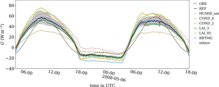
5308                             K. F. Gehrke et al.: Modeling of land–surface interactions in the PALM model system 6.0

    The PALM model system (formerly an abbreviation for            Section 5 outlines the results of the sensitivity study and
Parallelized Large-eddy Simulation Model; Maronga et al.,          discusses the validity and limitations of the LSM. Finally,
2015, 2020) has been applied for studying a variety of at-         Sect. 6 draws the summary and conclusions and gives an out-
mospheric boundary-layer flows for about 20 years. Since           look.
2015, PALM has come with a fully interactive LSM. Origi-
nally, it was designed similar to the LSM in the large-eddy
simulation (LES) model DALES (Heus et al., 2010), which            2     Description of the land surface model (LSM) in
contains parameterizations from the TESSEL/HTESSEL                       PALM
scheme (Viterbo and Beljaars, 1995; van den Hurk et al.,
                                                                   The specific implementation of PALM’s LSM, which is de-
2000; Balsamo et al., 2009, 2011), but also some found in
                                                                   rived from the HTESSEL scheme, is described below. It con-
the ISBA model (Noilhan and Mahfouf, 1996) and own ex-
                                                                   sists of a solver for the energy balance of the Earth’s surface
tensions. The LSM in PALM was first described by Maronga
                                                                   in combination with a multilayer soil scheme. The scheme
and Bosveld (2017) and has been used with respect to radia-
                                                                   was initially designed for vegetated surfaces and bare soil
tion fog by Maronga and Bosveld (2017) and Schwenkel and
                                                                   only, but it has since been adapted for paved surface materi-
Maronga (2019), also including Cabauw (Netherlands) data
                                                                   als like asphalt and concrete; a simplified version for inland
for evaluation. Recently, it has also been employed in urban
                                                                   and seawater surfaces has also been added. A tile approach
environments (see first results in Maronga et al., 2020).
                                                                   is available for vegetated surfaces, in which the surface is a
    Other coupled LES–LSM implementations are found in,
                                                                   fraction of bare soil and a fraction covered with vegetation.
e.g., UCLA-LES (Huang et al., 2011), ICON-LEM (Di-
                                                                   Furthermore, the LSM has a liquid water reservoir on plants
pankar et al., 2015), and the WRF model (Skamarock et al.,
                                                                   and soil to store and evaporate liquid water from precipita-
2019) in LES mode coupled to NOAH-LSM (Chen and Dud-
                                                                   tion interception and dew formation. A liquid water reservoir
hia, 2001). In early literature, the focus of coupled LES–LSM
                                                                   is also available when the surface type is set to pavement,
studies was mainly to analyze the feedback effect that cre-
                                                                   representing the ability of impervious surfaces to store a lim-
ates heterogeneity at the surface (e.g. Patton et al., 2005;
                                                                   ited amount of precipitated water on the surface. For further
Huang et al., 2009; Huang and Margulis, 2010; Brunsell
                                                                   details, see also Viterbo and Beljaars (1995), van den Hurk
et al., 2011). Today, most studies require the coupled LES–
                                                                   et al. (2000), Balsamo et al. (2009, 2011), and the literature
LSM approach to simulate realistic cases, e.g., in the ur-
                                                                   referenced therein.
ban environment or for wind turbine applications. As the
methodology gains a foothold in engineering and industry,          2.1    Energy balance solver
it is becoming increasingly important for the embedded land
surface representation in PALM to reflect reality (Maronga         The energy balance is calculated as
et al., 2020).
                                                                   dT0
    This paper is part of a series featuring different parts of         C0 = Rn − H − LE − G,                                    (1)
the PALM model system 6.0 in this special issue. For the             dt
user, a systematic sensitivity test of relevant land surface pa-   where C0 and T0 are the heat capacity and radiative temper-
rameters with the LSM in PALM is of particular interest.           ature of the surface, respectively. Note that C0 is zero by de-
In the present study, we evaluate the LSM embedded into            fault in the case of surfaces covered by vegetation or water
PALM against Cabauw data for a selected period with clear-         surfaces, for which it is assumed that T0 is the temperature
sky conditions and limited large-scale advection. Through          of a skin layer covering the surface that does not have a sig-
this we ensure as far as possible that the developing bound-       nificant heat capacity, which we think is a valid approach for
ary layer is not affected by non-local processes, which we         low vegetation like grass. The heat capacity is fully customiz-
neglect in the simulations of this study. Furthermore, we de-      able by the user and can be adjusted to account for the heat
termine key parameters that influence the diurnal cycle in a       stored in, e.g., forests (Lindroth et al., 2010; Swenson et al.,
coupled LES–LSM framework. The model sensitivity is an-            2019). In all other cases (i.e., pavements and bare soils), no
alyzed by means of a comprehensive set of simulations vary-        skin layer is assumed (see below). Rn , H , LE, and G are the
ing land surface and soil parameters individually. Therewith,      net radiation, sensible heat flux, latent heat flux, and ground
the present study complements the earlier work of Maronga          (soil) heat flux at the surface, respectively. Rn is defined pos-
and Bosveld (2017), who focused on the nocturnal boundary          itive downwards, whereas H , LE, and G are defined positive
layer with developing radiation fog.                               away from the surface. Rn is defined through the sum of the
    Section 2 of the paper describes physical and technical as-    radiative fluxes:
pects of the LSM in PALM. Section 3 provides information
                                                                   Rn = SW↓ − SW↑ + LW↓ − LW↑ ,                                 (2)
about the Cabauw Experimental Site for Atmospheric Re-
search (CESAR; Monna and Bosveld, 2013) and the obser-             where SW↓ , SW↑ , LW↓ , and LW↑ are the shortwave incom-
vations used. Section 4 describes the model setup and initial-     ing (downward), shortwave outgoing (upward), longwave in-
ization and gives a complete list of simulations conducted.        coming (downward), and longwave outgoing (upward) flux,

Geosci. Model Dev., 14, 5307–5329, 2021                                             https://doi.org/10.5194/gmd-14-5307-2021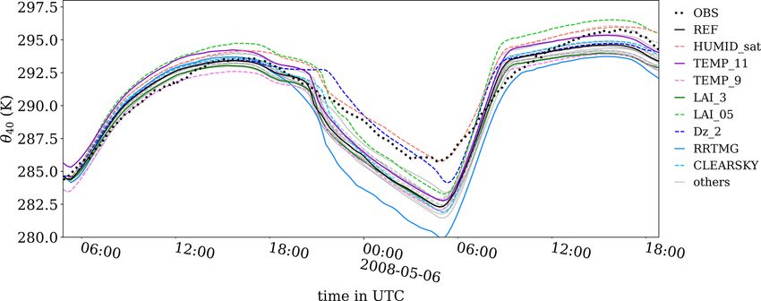
K. F. Gehrke et al.: Modeling of land–surface interactions in the PALM model system 6.0                                       5309

respectively. The radiation components are defined positive        soil layer:
according to their direction (SW↓ and LW↓ positive down-
wards; SW↑ and LW↑ positive upwards). The radiative fluxes              λT,pave
                                                                   3=            ,                                              (8)
are provided by one of the available radiation schemes in               1zsoil,1
PALM (for details, see Maronga et al., 2020).
                                                                   with λT,pave being the thermal conductivity of the pavement
2.1.1     Parameterization of fluxes                               and 1zsoil,1 being the thickness of the uppermost soil layer.
                                                                   In this case, it is assumed that the soil temperature is constant
The turbulent heat fluxes are both parameterized using a re-       within the uppermost 25 % of the topsoil layer and equals
sistance parameterization. H is calculated as                      the radiative temperature at the surface. C0 is then set to a
                                                                   nonzero value according to the material properties and the
              1                                                    layer thickness.
H = −ρcp         (θmo − θ0 ),                               (3)
              ra                                                      The total latent heat flux, LE, is parameterized as
where ρ is the density of the air, cp = 1005 J kg−1 K−1 is the                      1
specific heat at constant pressure, and ra is the aerodynamic      LE = −ρlv             (qv,mo − qv,sat (T0 )).                (9)
                                                                                 ra + rs
resistance. θ0 and θmo are the potential temperature at the
surface and at a fixed height within the atmospheric surface       Here, lv = 2.5 × 10⁶ J kg−1 is the latent heat of vaporization,
layer (at height zmo , usually at the height of the first atmo-    rs is the total surface resistance, qmo is the water vapor mix-
spheric grid level, i.e., zmo = 0.51z , where 1z is the verti-     ing ratio at height zmo , and qsat is the water vapor mixing
cal grid spacing), respectively. The potential temperature is      ratio at saturation at the surface, which is a function of T0 .
linked to the actual temperature via the Exner function:           In practice, up to three individual components are calculated
                                                                   for vegetated surfaces. Transpiration of the vegetated fraction
          p     Rd /cp
5=                       ,                                   (4)   (LEveg ) is parameterized as
        1000 hPa
where p is the pressure and Rd is the gas constant for dry                              1
                                                                   LEveg = −ρlv              (qv,mo − qv,sat (T0 )),           (10)
air. ra is calculated via Monin–Obukhov similarity theory                            ra + rc
(MOST) as
                                                                   where rc is the canopy resistance. Analogously, the bare soil
     θmo − θ0                                                      fraction evaporation (LEsoil ) is calculated via
ra =          ,                                             (5)
       u∗ θ∗
                                                                                         1
where u∗ and θ∗ are the friction velocity and characteristic       LEsoil = −ρlv                (qv,mo − qv,sat (T0 )),        (11)
                                                                                     ra + rsoil
temperature scale, respectively. These values are calculated
locally using MOST. The roughness lengths are individually         with rsoil being the soil resistance. The liquid water reservoir
set for momentum, heat, and moisture (see Table 1). Note that      evaporation (LEliq ) is given by
ra in Eq. (5) is calculated based on u∗ and θ∗ values from
                                                                                     1
the current time step to calculate H at the prognostic time        LEliq = −ρlv         (qv,mo − qv,sat (T0 ));                (12)
step. For details on the particular implementation of MOST                           ra
in PALM, see Maronga et al. (2020).                                i.e., only the aerodynamic resistance exists for liquid water.
   The ground heat flux, G, is parameterized after Duynkerke       The total evapotranspiration is then given by a combination
(1999) as                                                          of the three individual components by (see Viterbo and Bel-
G = 3(T0 − Tsoil,1 ),                                       (6)    jaars, 1995)

with 3 being the total thermal conductivity between the skin       LE =cveg (1 − cliq )LEveg + cliq LEliq
layer and the uppermost soil layer. Tsoil,1 is the temperature            + (1 − cveg )(1 − cliq )LEsoil .                     (13)
of the uppermost soil layer (calculated at the center of the
layer). 3 is calculated via a resistance approach as a combi-      Here, cveg and cliq are the fractions of the surface covered
nation of the conductivity between the canopy and the soil         with vegetation and liquid water, respectively. Liquid water
top (3skin , constant value) and the conductivity of the top       from precipitation can be stored on the vegetation and bare
half of the uppermost soil layer (3soil ):                         soil. Note that for paved and water surfaces both LEveg and
                                                                   LEsoil are set to zero and the only possible source of evapo-
         3skin 3soil                                               ration is the liquid water reservoir.
3=                    .                                     (7)
        3skin + 3soil                                                 All equations above are solved locally for each surface el-
When no skin layer is used (i.e., for pavements and bare           ement of the model grid.
soils), 3 simplifies to the heat conductivity of the uppermost

https://doi.org/10.5194/gmd-14-5307-2021                                                Geosci. Model Dev., 14, 5307–5329, 2021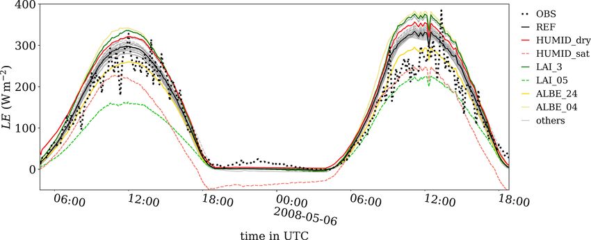
5310 K. F. Gehrke et al.: Modeling of land–surface interactions in the PALM model system 6.0
Table 1. Lookup table for vegetation parameters of 18 predefined vegetation types in the style of the ECMWF classification, adapted for
PALM. 3skin,s and 3skin,u are the total thermal conductivities between the skin layer and the surface for near-surface stable and unstable
stratification, respectively. is the surface emissivity. All other symbols are used as defined in the main text.
Type Description rc,min LAI cveg gD z0 z0,h 3skin,s 3skin,u C0 Albedo type
(m s−1 ) (hPa−1 ) (m) (m) (W m−2 K−1 ) (W m−2 K−1 )
1 bare soil 0.0 0.00 0.00 0.00 0.005 0.5 × 10⁻⁴ 0.0 0.0 0.00 17 0.94
2 crops, mixed farming 180.0 3.00 1.00 0.00 0.10 0.001 10.0 10.0 0.00 2 0.95
3 short grass 110.0 2.00 1.00 0.00 0.03 0.3 × 10⁻⁴ 10.0 10.0 0.00 5 0.95
4 evergreen needleleaf trees 500.0 5.00 1.00 0.03 2.00 2.00 20.0 15.0 0.00 6 0.97
5 deciduous needleleaf trees 500.0 5.00 1.00 0.03 2.00 2.00 20.0 15.0 0.00 8 0.97
6 evergreen broadleaf trees 175.0 5.00 1.00 0.03 2.00 2.00 20.0 15.0 0.00 9 0.97
7 deciduous broadleaf trees 240.0 6.00 0.99 0.13 2.00 2.00 20.0 15.0 0.00 7 0.97
8 tall grass 100.0 2.00 0.70 0.00 0.47 0.47 × 10⁻² 10.0 10.0 0.00 10 0.97
9 desert 250.0 0.05 0.00 0.00 0.013 0.013 × 10⁻² 15.0 15.0 0.00 11 0.94
10 tundra 80.0 1.00 0.50 0.00 0.034 0.034 × 10⁻² 10.0 10.0 0.00 13 0.97
11 irrigated crops 180.0 3.00 1.00 0.00 0.5 0.50 × 10⁻² 10.0 10.0 0.00 2 0.97
12 semidesert 150.0 0.50 0.10 0.00 0.17 0.17 × 10⁻² 10.0 10.0 0.00 11 0.97
13 ice caps and glaciers 0.0 0.00 0.00 0.00 1.3 × 10⁻³ 1.3 × 10⁻⁴ 58.0 58.0 0.00 14 0.97
14 bogs and marshes 240.0 4.00 0.60 0.00 0.83 0.83 × 10⁻² 10.0 10.0 0.00 3 0.97
15 evergreen shrubs 225.0 3.00 0.50 0.00 0.10 0.10 × 10⁻² 10.0 10.0 0.00 4 0.97
16 deciduous shrubs 225.0 1.50 0.50 0.00 0.25 0.25 × 10⁻² 10.0 10.0 0.00 5 0.97
17 mixed forest–woodland 250.0 5.00 1.00 0.03 2.00 2.00 20.0 15.0 0.00 10 0.97
18 interrupted forest 175.0 2.50 1.00 0.03 1.10 1.10 20.0 15.0 0.00 7 0.97
2.1.2 Liquid water reservoir (edef = esat −e, with esat and e being the water vapor pressure
at saturation and the current water vapor pressure, respec-
To account for the evaporation of liquid water on plants and tively). The layer-averaged volumetric soil moisture content
impervious surfaces, an additional equation is solved for the (m̃) is given by
liquid water reservoir:
N
X
dmliq LEliq m̃ = Rfr,k max(msoil,k , mwilt ), (17)
= , (14)
dt ρl lv k=1
where mliq and ρl are the water column on the surface and where N is the number of soil layers, Rfr,k is the root fraction
the density of water, respectively. The maximum amount of in layer k, msoil,k is the volumetric soil moisture content in
water that can be stored on plants is calculated via layer k, and mwilt is the permanent wilting point.
mliq,max = min 1, mliq,ref · (cveg · LAI + (1 − cveg )) , (15) The correction functions f1 is
where mliq,ref = 0.2 mm is the reference liquid water col- 1 0.004SW↓
= min 1, , (18)
umn on a single leaf or bare soil and LAI the leaf area in- f1 (SW↓ ) 0.81(0.004SW↓ + 1)
dex. Excess liquid water is directly removed from the sur- which accounts for the reaction of plants to sunlight (opening
face and infiltrated in the underlying soil. For paved sur- and closing stomatas); the reaction of plants to water avail-
faces, mliq,max is set to 1 mm. Excess liquid water is as- ability in the soil is given by the correction function f2 as
sumed to be drained off. Note that mliq enters the calcula-
tion of LEliq indirectly via cliq , which is given either as the 0
m̃ < mwilt
ratio mliq /mliq,max for vegetation (following the HTESSEL 1 m̃−mwilt
= m −m mwilt ≤ m̃ ≤ mfc (19)
scheme) or (mliq /mliq,max )0.67 for pavement following Mas- f2 (m̃) fc wilt
son (2000) (based on Noilhan and Planton, 1989). 1 m̃ > mfc ,
with mfc being the soil moisture at field capacity. Further-
2.1.3 Calculation of resistances
more, a correction for the water vapor pressure deficit is
The resistances are calculated separately for bare soil and given by
vegetation following Jarvis (1976). The canopy resistance, 1
rc , is calculated as = exp(gD edef ), (20)
f3 (edef )
rc,min
rc = f1 (SW↓ )f2 (m̃)f3 (edef ), (16) where gD is a correction factor that is used for tall vegetation
LAI
such as trees.
with rc,min being a minimum canopy resistance. f1 − f3 are The soil resistance (rsoil ) is calculated as
correction functions that depend on LAI, the incoming short-
wave radiation (SW↓ ), and the water vapor pressure deficit rsoil = rsoil,min · f4 msoil,1 , (21)
Geosci. Model Dev., 14, 5307–5329, 2021 https://doi.org/10.5194/gmd-14-5307-2021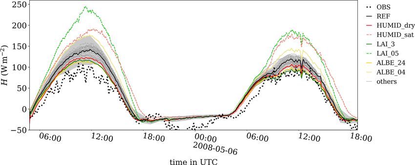
K. F. Gehrke et al.: Modeling of land–surface interactions in the PALM model system 6.0                                      5311

where rsoil,min is the minimum soil resistance. The correction      At the bottom boundary a fixed deep soil temperature Tdeep is
function f4 is given by                                             prescribed (Dirichlet conditions). The user must ensure that
                                                                  the soil model reaches deep enough such that atmospheri-
             msoil,1 − mmin                                         cally driven temperature changes do not propagate down to
f4 = max                    ,1 ,                          (22)
              mfc − mmin                                            the boundary condition.
with mmin being a minimum soil moisture for the soil matrix         2.2.2    Soil moisture transport
based on the wilting point and the residual moisture mres ,
calculated as                                                       The vertical transport of water within the soil matrix is cal-
                                                                    culated using Richards’ equation:
mmin = cveg mwilt + (1 − cveg )mres .                       (23)
                                                                    ∂msoil     ∂      ∂msoil
  Note that the total surface resistance (rs , see Eq. 9) is cal-          =       λm         − γ + Sm ,                     (28)
                                                                      ∂t      ∂z        ∂z
culated as a diagnostic quantity from LE after the energy
balance is solved.                                                  where λm , γ , and Sm are the hydraulic diffusion coefficient,
                                                                    hydraulic conductivity, and a sink term due to root extraction,
2.2     Soil model                                                  respectively. The hydraulic diffusion coefficient is calculated
                                                                    after Clapp and Hornberger (1978) as
Prognostic equations for the soil temperature and the volu-
metric soil moisture are solved in multiple layers in the soil              bγsat (−9sat ) msoil b+2

model. Transport is restricted to only the vertical direction       λm =                             ,                        (29)
                                                                                msat        msat
within the soil, and no ice phase is currently considered. By
default, the soil model is constructed of eight layers, with        with b = 6.04 being a fixed parameter, γsat being the hy-
default layer thicknesses of 0.01, 0.02, 0.04, 0.06, 0.14, 0.26,    draulic conductivity at saturation, and 9sat = −338 m being
0.54, and 1.86 m; however, the number and thicknesses of            the soil matrix potential at saturation. The hydraulic con-
layers are fully customizable. The vertical heat and water          ductivity (γ ) is calculated after van Genuchten (1980) (as in
transport is modeled using the Fourier law of diffusion and         HTESSEL):
Richards’ equation, respectively. For vegetated surface ele-                                              2
                                                                              (1 + (αh)n )1−1/n − (αh)n−1

ments, root fractions are assigned to each soil layer to ac-
                                                                    γ = γsat                                 .                (30)
count for the explicit withdrawal of water by plants, used for                   (1 + (αh)n )(1−1/n)(l+2)
transpiration, from the respective soil layer. Viterbo and Bel-
jaars (1995) and Balsamo et al. (2009) give more details.           Here, α, n, and l are van Genuchten coefficients that depend
                                                                    on the soil type (see Table 2). h is the pressure head, which
2.2.1    Soil heat transport                                        is calculated via rearrangement of

The Fourier law of diffusion is                                                                msat − mres
                                                                    msoil (h) = mres +                        .               (31)
                                                                                          (1 + (αh)n )1−1/n
         ∂Tsoil   ∂       ∂Tsoil
(ρC)soil        =      λT          ,                        (24)
          ∂t      ∂z       ∂z                                         The root extraction of water from the respective soil layer,
with (ρC)soil and λT being the volumetric heat capacity and         Sm,k , is calculated as follows:
the thermal conductivity of a soil layer, respectively. λT is                 LEveg Rfr,k msoil,k
calculated as                                                       Sm,k =                           ,                        (32)
                                                                               ρl lv 1zsoil,k mtotal
λT = Ke(λT,sat − λT,dry ) + λT,dry ,                        (25)    where mtotal is the total water content of the soil,
with λT,sat , λT,dry , and Ke being the thermal conductivity of                N
                                                                               X
saturated soil, the thermal conductivity of dry soil, and the       mtotal =         Rfr,k msoil,k ,                          (33)
Kersten number, respectively. λT,sat is given by                               k=1

            1−m                                                     with Rfr,k being the root fraction in soil layer k. Only the
λT,sat = λT,smsoil,sat λm .                                 (26)
                                                                    layers that have a soil moisture above the wilting point are
Here, λT,sm is the thermal conductivity of the soil matrix and      used in Eq. (33) (i.e., plants are unable to withdraw water
λm is the heat conductivity of water. The Kersten number            from layers with soil moisture below the wilting point). The
(Ke) is calculated as                                               root distribution within the soil must be chosen such that
                                                                N
                        msoil
                                                                    X
Ke = log10 max 0.1,              + 1.                     (27)            Rfr,k = 1.                                          (34)
                        msat                                        k=1

https://doi.org/10.5194/gmd-14-5307-2021                                                   Geosci. Model Dev., 14, 5307–5329, 2021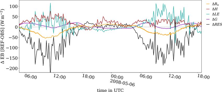
5312                                    K. F. Gehrke et al.: Modeling of land–surface interactions in the PALM model system 6.0

Table 2. Lookup table for soil parameters.

             Type       Description             α              l         n               γsat             msat          mfc         mwilt            mres
                                                                                     (m s−1 )         (m3 s−3 )    (m3 s−3 )     (m3 s−3 )       (m3 s−3 )
             1          coarse               3.83       1.150        1.38      6.94 × 10⁻⁶               0.403        0.244         0.059           0.025
             2          medium               3.14      −2.342        1.28      1.16 × 10⁻⁶               0.439        0.347         0.151           0.010
             3          medium–fine          0.83      −0.588        1.25      0.26 × 10⁻⁶               0.430        0.383         0.133           0.010
             4          fine                 3.67      −1.977        1.10      2.87 × 10⁻⁶               0.520        0.448         0.279           0.010
             5          very fine            2.65       2.500        1.10      1.74 × 10⁻⁶               0.614        0.541         0.335           0.010
             6          organic              1.30       0.400        1.20      1.20 × 10⁻⁶               0.766        0.663         0.267           0.010

Table 3. Lookup table for albedo parameters.

                   Albedo type         Description                                          Broadband         Longwave         Shortwave     Notes
                   1                   ocean                                                          0.06           0.06           0.06
                   2                   mixed farming, tall grassland                                  0.19           0.28           0.09
                   3                   tall–medium grassland                                          0.23           0.33           0.11
                   4                   evergreen shrubland                                            0.23           0.33           0.11
                   5                   short grassland, meadow, shrubland                             0.25           0.34           0.14
                   6                   evergreen needleleaf forest                                    0.14           0.22           0.06
                   7                   mixed deciduous forest                                         0.17           0.27           0.06
                   8                   deciduous forest                                               0.19           0.31           0.06
                   9                   tropical evergreen broadleaved forest                          0.14           0.22           0.06
                   10                  medium–tall grassland and woodland                             0.18           0.28           0.06
                   11                  desert, sandy                                                  0.43           0.51           0.35
                   12                  desert, rocky                                                  0.32           0.40           0.24
                   13                  tundra                                                         0.19           0.27           0.10
                   14                  land ice                                                       0.77           0.65           0.90     1
                   15                  sea ice                                                        0.77           0.65           0.90
                   16                  snow                                                           0.82           0.70           0.95
                   17                  bare soil                                                      0.08           0.08           0.08
                   18                  asphalt–concrete mix                                           0.17           0.17           0.17     2
                   19                  asphalt (asphalt concrete)                                     0.17           0.17           0.17     2
                   20                  concrete (Portland concrete)                                   0.30           0.30           0.30     2
                   21                  sett                                                           0.17           0.17           0.17     2
                   22                  paving stones                                                  0.17           0.17           0.17     2
                   23                  cobblestone                                                    0.17           0.17           0.17     2
                   24                  metal                                                          0.17           0.17           0.17     2
                   25                  wood                                                           0.17           0.17           0.17     2
                   26                  gravel                                                         0.17           0.17           0.17     2
                   27                  fine gravel                                                    0.17           0.17           0.17     2
                   28                  pebblestone                                                    0.17           0.17           0.17     2
                   29                  woodchips                                                      0.17           0.17           0.17     2
                   30                  tartan (sports)                                                0.17           0.17           0.17     2
                   31                  artificial turf (sports)                                       0.17           0.17           0.17     2
                   32                  clay (sports)                                                  0.17           0.17           0.17     2
                   33                  building (dummy)                                               0.17           0.17           0.17     2

                 1 Land ice is treated differently than sea ice. 2 Preliminary and/or dummy values.

Geosci. Model Dev., 14, 5307–5329, 2021                                                                           https://doi.org/10.5194/gmd-14-5307-2021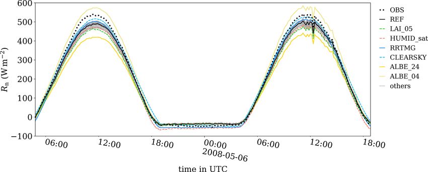
K. F. Gehrke et al.: Modeling of land–surface interactions in the PALM model system 6.0                                   5313

   There are two options for the soil moisture bottom bound-      a diagnostic relationship:
ary condition. The bottom surface can be set to bedrock; i.e.,
water is not drained. Instead, it is accumulated in the low-                A
                                                                  T0t+1 =     .                                            (38)
est soil layer (water content conservation). Alternatively, the             B
bottom boundary can be set to free drainage, i.e., an open bot-
tom where soil water is continuously lost by drainage (water      3   CESAR observations
content is not conserved).
                                                                  For model evaluation we simulate 2 consecutive clear-sky
2.2.3    Treatment of pavements                                   days observed on 5 and 6 May 2008 at the CESAR site
                                                                  near Cabauw. This period is used because the forcing from
Pavements are treated identically to soil (allowing varying       the surface was dominant and larger-scale advection is lim-
numbers and depths of the pavement layers) but with the           ited. We decided to simulate a 2 d period to study the behav-
physical properties of the pavement material. The pavement        ior of the model over a full diurnal cycle and also look at
layer is impermeable to water, which prohibits the vertical       how the first day affects the following day. With a longer pe-
transport of soil moisture. Soil layers are placed below the      riod, model drift must be taken care of by, e.g., adding nudg-
pavement layers.                                                  ing to the forcing and/or data assimilation. This would add
                                                                  additional uncertainty because height-dependent advection,
2.2.4    Treatment of water bodies
                                                                  which is needed to drive the LES model, is difficult or im-
For water surfaces, PALM currently only allows prescrip-          possible to obtain from observations, particularly within the
tion of a bulk water temperature. The energy balance is then      boundary layer where turbulence dominates.
solved as for land surfaces but without evapotranspiration           As part of the IMPACT-EUCAARI campaign in May 2008
from vegetation and bare soil (see above). A skin layer is        (Intensive Measurement Period at the Cabauw Tower within
adopted to calculate the heat flux into the water body, with      the European Integrated project on Aerosol Cloud Climate
C0 = 0 J m−2 K−1 and 3 = 1 × 10¹¹ W m2 K−1 .                      and Air Quality Interactions; Kulmala et al., 2009), radioson-
   In the case of an ocean surface, a Charnock parameteriza-      des were launched daily at 05:00, 10:00, and 16:00 UTC,
tion can be switched on to account for the effect of waves        which we use to initialize the simulations. CESAR features
on the surface friction in terms of a modification of the sur-    a 213 m high measurement mast with instruments at 1.5, 10,
face roughness length as described by Beljaars (1994). For        20, 40, 80, 140, and 200 m (Bosveld, 2020). For our model
details, see Maronga et al. (2020).                               comparison, we use 10 min averages of temperature, specific
                                                                  humidity, and horizontal wind speed. The measurement ac-
2.3     Numerical methods                                         curacy for temperature and humidity is 0.1 K and 3.5 %, re-
                                                                  spectively (Meijer, 2000). The accuracy for horizontal wind
To solve the energy balance for the surface temperature (T0 ),    speed is the largest of either 1 % or 0.1 m s−1 . Soil temper-
Eq. (1) is first linearized around T0 at the current time step    ature is observed at a depth of 0, 2, 4, 6, 8, 12, 20, 30,
and then discretized in time using PALM’s default Runge–          and 50 cm. The surface soil heat flux is computed from soil
Kutta third-order time-stepping scheme. With this method,         heat flux measurements at 5 and 10 cm depths by means of
an iterative procedure to solve the energy balance is avoided.    a Fourier extrapolation (see Bosveld, 2020, variable FG0 in
The prognostic equation then reads                                their Ch. 19). Net radiation is calculated from the budget of
                                                                  the four radiation components (see Eq. 2). Turbulent fluxes of
          A1t + C0 T0t
T0t+1 =                ,                                   (35)   sensible and latent heat are computed by means of the eddy
           C0 + B1t                                               covariance (EC) method. In the process of calculating EC
where t is the time index and 1t is the current time step. A      fluxes from raw turbulence data it is unavoidable that low-
and B are coefficients given by                                   frequency contributions to the flux are not represented. For
                                                                the Cabauw data, the 10 min means are subtracted from the
                      ρcp                                         raw turbulent time series; thereafter, a low-frequency correc-
A = Rn + 3σ T04 +           θmo                         (36)
                       ra                                         tion is applied based on the spectra by Kaimal et al. (1972),
                                                                  with dependence on wind speed and stability (Fred Bosveld,

            ρlv                   dqsat
     +               qmo − qsat +       T0 + 3Tsoil,1             personal communication, 2020). The low-frequency loss cor-
          ra + rs                  dT
                                                                  rection assumes that all turbulence characteristics follow
and                                                               surface-layer scaling. However, this is not always true. For
                                                                  example, horizontal advection by organized turbulent struc-

                 ρlv         dqsat     ρcp
B = 3+                             +          + 4σ T03 .   (37)   tures (Eder et al., 2015; De Roo and Mauder, 2018) may add
               ra + rs        dT       ra 5
                                                                  further low-frequency contributions that are not accounted
Here, σ = 5.67037×10⁻⁸ is the Stefan–Boltzmann constant.          for in the surface-layer scaling. For further information on
For vegetated surfaces, where C0 is zero, Eq. (35) reduces to     the instrumentation of the Cabauw site, see Bosveld (2020).

https://doi.org/10.5194/gmd-14-5307-2021                                            Geosci. Model Dev., 14, 5307–5329, 2021
5314 K. F. Gehrke et al.: Modeling of land–surface interactions in the PALM model system 6.0
surface is “short grass” with some modifications. The rough-
ness length for momentum is set to 0.15 m, which is repre-
sentative for a few kilometers of upstream terrain from the
Cabauw tower, and the roughness length for temperature is
set to 2.35 × 10⁻⁵ m (Ek and Holtslag, 2004). The soil layers
are defined at depths of 0.005, 0.02, 0.04, 0.065, 0.1, 0.15,
0.24, 0.45, 0.675, 1.125, and 2.25 m. The soil parameters for
field capacity and wilting point are 0.491 and 0.314, respec-
tively, which is consistent with a very fine soil texture. The
deep soil temperature is fixed at 283.19 K, which is a valid as-
sumption because the lower two soil levels are not reached by
diurnal temperature variations (lower part of Fig. 1 does not
change over time). The van Genuchten coefficients, the hy-
draulic conductivity at saturation, and the porosity vary with
soil depth. In the uppermost 24 cm, the parameters are set
to match medium–fine soil (type 3 in Table 2). The layer be-
tween 24 and 60 cm is identical to the uppermost layer except
for the porosity, which is increased due to observed large val-
ues of soil moisture. Between 60 and 225 cm, the parameters
Figure 1. Vertical soil layer setup of root density (Rdens , a) as well are set to organic soil according to Table 2. In all simulations,
as initial profiles of temperature (b) and moisture (c). Note the bro- the land surface and soil parameters are homogeneous over
ken vertical axis with a changed linear increment in the deeper lay- the model domain. This means that buildings in the small
ers. The root fraction of each soil layer (see Rfr in Table 4) is the
town of Lopik, west of the CESAR tower, are neglected, as
difference of the cumulative root fraction (Eq. 34; shown on the
are the small ditches that cross the observation site.
vertical axis) between two layers.
The root fraction and initial soil profiles of temperature
and moisture are shown in Fig. 1. The root density is based
Cabauw is located in the western part of the Netherlands. on the study of Jager et al. (1976), who describe the vertical
It is surrounded primarily by meadows with ditches, villages, structure as follows. A layer of relatively high root density,
orchards, and lines of trees. The CESAR tower itself is in- Rdens , extends from 3 cm below the surface down to 18 cm,
stalled over an area of short grass that is kept at a height followed by a layer of relatively low root density down to
of approximately 8 cm. The immediate surroundings of the 60 cm of depth. No roots are found near the surface (< 3 cm)
measuring tower are free of significant heterogeneities for and in the deep soil layers (> 60 cm). The initial soil temper-
a few hundred meters. During the simulation period from 5 ature and moisture profiles are taken from measurement data
to 6 May 2008 the prevailing wind direction was from the on 5 May 2008 at 05:00 UTC (shown in Fig. 1). A summary
southeast, and the 10 m average wind speed ranged from 2 of the land surface scheme configuration is listed in Table 4.
to 6 m s−1 . The convective boundary layer reached a height Case REF is driven by external forcing of incoming short-
of approximately 2 km. The groundwater level was 1.3 m in wave and longwave radiation taken from the Cabauw mea-
depth. The soil temperature, Tsoil , and soil moisture, msoil , on surements. The effects of high-altitude aerosols, moisture,
5 May 2008 at 05:00 UTC are depicted in Fig. 1 (see Sect. 4). and clouds are included in this forcing. Accordingly, the de-
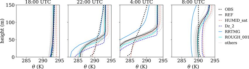
The profiles of temperature θ , humidity q, and horizontal grees of freedom are reduced and we can focus on parame-
wind vh retrieved from radiosounding are shown in Fig. 2 ters of the LSM rather than additional uncertainties of a ra-
together with tower measurements from all available levels diation model. Nonetheless, we performed sensitivity tests
(see details in Sect. 5). using the Rapid Radiation Transfer Model for Global Mod-
els (RRTMG; Clough et al., 2005) and a clear-sky radiation
parameterization, which are described in detail in Maronga
4 Simulation setup et al. (2020). The longwave outgoing radiation of the sur-
face is calculated from the skin layer temperature using the
The CESAR site is well-equipped with vegetation and soil Stefan–Boltzmann law. The longwave and shortwave albedos
information (e.g., Beljaars and Bosveld, 1997), which pro- for diffusive radiation are set to 0.34 and 0.14, respectively, to
vides a good opportunity to evaluate the land surface param- fit the dominating grassland. Albedos for direct radiation are
eterization proposed in the present study. The reference sim- calculated according to Briegleb (1992) considering a weak
ulation (hereafter referred to as case REF) was set up as a solar zenith angle dependence such that their direct values
best guess with the Cabauw land surface parameters accord- equal the diffusive ones at 60◦ .
ing to Beljaars and Bosveld (1997), Ek and Holtslag (2004), The model domain for case REF is (x × y × z) 2000 m ×
and Maronga and Bosveld (2017). The vegetation type of the 2000 m × 4317 m with a horizontal and vertical grid spacing
Geosci. Model Dev., 14, 5307–5329, 2021 https://doi.org/10.5194/gmd-14-5307-2021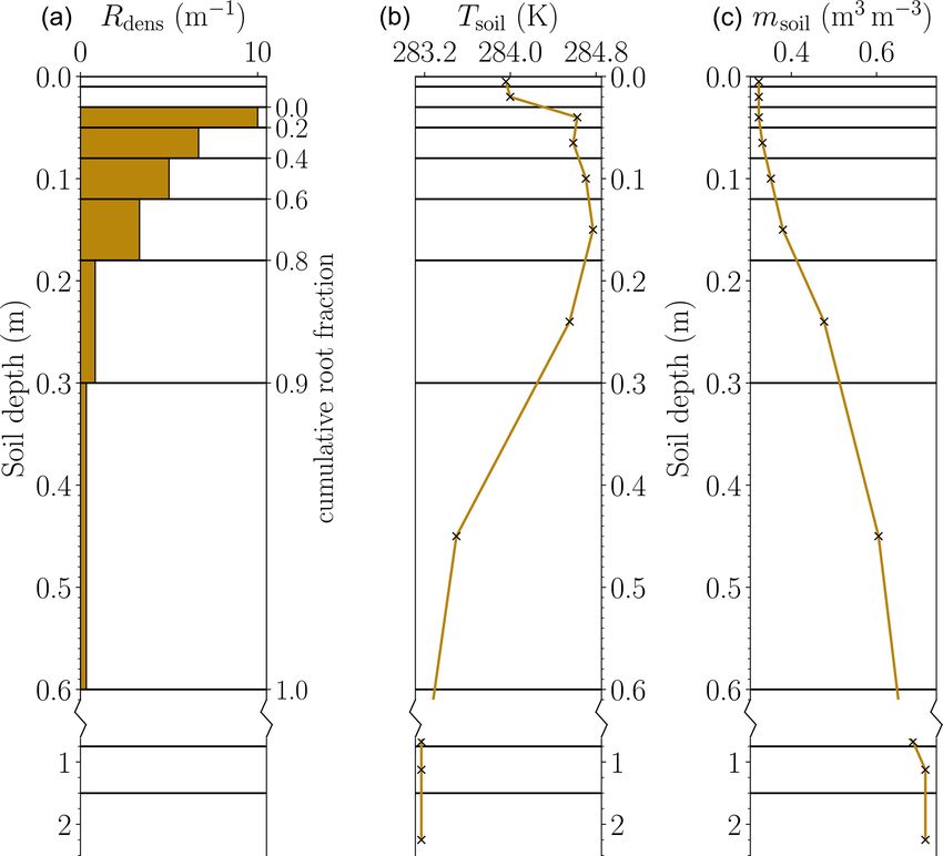
K. F. Gehrke et al.: Modeling of land–surface interactions in the PALM model system 6.0                                                5315

Figure 2. Vertical profiles of θ , q, and vh measured by radiosonde (dashed lines) and the tower (point markers) at the CESAR site as well as
simulated profiles of case REF (continuous lines) during the 2 d period. Note that the lower 300 m is shown with a higher vertical resolution
than the layers above to better visualize individual tower measurements (the black horizontal line indicates the break).

of 50 and 10 m, respectively. A grid sensitivity study is car-           available, imposing rather high uncertainty on these data. An
ried out to justify this grid spacing (see Sect. 5). Above the           overview of the sensitivity simulations and their well-defined
boundary layer (> 2000 m), a vertical grid stretching is ap-             change compared to case REF is given in Table 5.
plied with a stretching factor of 1.08 and a maximum ver-
tical grid spacing of 100 m. Initial profiles of temperature,
humidity, and horizontal wind for case REF are taken from                5     Results
radiosounding data and are shown in Fig. 2. The horizontal
wind equals the initial u component of the wind vector; i.e.,            5.1    Boundary-layer profiles
at the beginning of the simulation there is no wind turning
with height due to Coriolis force. The geostrophic wind at               At first, we will look at the vertical profiles of the radiosonde
the top of the domain is set to 7 and 0 m s−1 for the u and v            and tower measurements. Figure 2 shows vertical profiles of
component, respectively. The lateral boundary conditions are             θ , q, and vh , indicating the evolution of the boundary layer
cyclic.                                                                  during the considered period of time in Cabauw at the times
   In addition to simulation REF, sensitivity simulations are            of the radiosonde ascents. Both nights show a stable noctur-
performed. All sensitivity simulations are based on the ref-             nal boundary layer before sunrise (at 05:00 UTC). A night-
erence simulation and only differ by one specific parameter              time low-level jet is observed in the horizontal wind. Pro-
that is varied in a reasonable range. With these sensitivity             files of potential temperature and water vapor mixing ratio
simulations we do not intend to give a comprehensive pa-                 show a well-mixed convective boundary layer at 10:00 and
rameter study, which usually covers a wide range of param-               16:00 UTC on both days. Over the course of the 2 d, the depth
eters. Nonetheless, the simulations provide an idea of how               of the convective boundary layer increases. The profiles of
sensitively the model reacts to specific parameters or pro-              vh show a mismatch between the radiosounding measure-
cesses included. This is mainly motivated by the fact that in            ments and the tower data. This is explained by different anal-
many simulation setups the respective input data for the land            ysis timescales. The radiosonde records instantaneous values
surface parameters are often not available or only roughly               with a sampling frequency of 0.1 Hz, which results in five

https://doi.org/10.5194/gmd-14-5307-2021                                                     Geosci. Model Dev., 14, 5307–5329, 2021
5316                              K. F. Gehrke et al.: Modeling of land–surface interactions in the PALM model system 6.0

Table 4. Overview of the land surface scheme configuration for case REF.

   Parameter     Value                                                             Description
                                                          Skin layer parameters
   C0            0 J m−2 K−1                                                       Heat capacity of the skin layer
   cveg          100 %                                                             Vegetation coverage of the surface
   LAI           1.7 m2 m−2                                                        Leaf area index
   rc,min        110 s m−1                                                         Minimum canopy resistance
   z0            0.15 m                                                            Roughness length for momentum
   z0,h          2.35 × 10⁻⁵ m                                                     Roughness length for temperature
   3skin         4.0 W m2 K−1                                                      Heat conductivity between skin layer and soil
                0.97                                                              Surface emissivity
                                                             Soil parameters
   mres          0.010 m3 s−3                                                      Residual volumetric soil moisture
   rsoil,min     50 s m−1                                                          Minimum soil resistance
   Tdeep         283.19 K                                                          Deep soil temperature
   mfc           0.491 m3 s−3                                                      Volumetric soil moisture at field capacity
   mwilt         0.314 m3 s−3                                                      Volumetric soil moisture at permanent wilting point
                                      Height-dependent soil parameters (0–24, 24–60, 60–225 cm)
   α             0.83, 0.83, 1.30                                                  van Genuchten coefficient
   l             −0.588, −0.588, 0.400                                             van Genuchten coefficient
   n             1.25, 1.25, 1.20                                                  van Genuchten coefficient
   γsat          0.26, 0.26, 1.2 × 10⁻⁶ m s−1                                      Hydraulic conductivity of the soil at saturation
   msat          0.430, 0.766, 0.766 m3 s−3                                        Volumetric soil moisture at saturation (porosity)
                                                           Initial soil profiles
   Tsoil,k       283.96, 284.00, 284.62, 284.59, 284.70, 284.77, 284.55,           Soil temperature at depth level k(k ∈ 1, 11)
                 283.50, 283.19, 283.19, 283.19 K
   msoil,k       0.324, 0.324, 0.324, 0.332, 0.352, 0.380, 0.477, 0.605, 0.670,    Soil moisture at depth level k(k ∈ 1, 11)
                 0.721, 0.721 m3 m−3
   Rfr,k         0, 0, 0.2, 0.2, 0.2, 0.2, 0.1, 0.1, 0, 0, 0                       Root fraction at depth level k(k ∈ 1, 11)

recording heights below 300 m. Conversely, data from the                layer depth despite fairly good agreement of the model and
cup anemometers at the mast are temporally averaged over                observations regarding mixed-layer temperature and humid-
10 min based on a 3 s running mean calculated with an update            ity values. The wind profiles agree well with observations.
frequency of 4 Hz (Bosveld, 2020). Thus, the mean tower                 At night (6 May 2008, 05:00 UTC), the near-surface tem-
profiles can be overestimated or underestimated by the in-              perature is significantly lower (out of range at ca. 281 K)
stantaneous values of the radiosonde. Note that we initialize           than measured. Similar to the mixing layer, the simulation
the simulations with data from the radiosonde ascent because            also underestimates the nocturnal boundary-layer depth. At
it reaches high enough, but comparisons are made against                the same time, the near-surface humidity shows small dif-
tower data due to the higher temporal resolution.                       ferences between the model and reality. The simulated hori-
   Figure 2 also shows the vertical profiles of the reference           zontal wind speed also depicts a low-level jet, but compared
simulation, which are temporally averaged over 15 min and               with observations it occurs closer to the surface, in accor-
horizontally averaged over the whole domain. A compari-                 dance with the simulated nocturnal boundary-layer depth.
son of observed profiles of θ and q with those of the LES               Even though the LES cannot reproduce the nocturnal ob-
show that the boundary-layer depth is underestimated by the             servations precisely, the mixed layer quickly develops the
simulation at 10:00 UTC on the first day. One hypothesis to             next morning (6 May 2008, 10:00 UTC), which is in agree-
explain this is that the turbulence development during model            ment with findings of van Stratum and Stevens (2015). At
spin-up, i.e., on the first morning, takes longer than in reality.      10:00 UTC on the second day, the simulation indicates a
The horizontal wind speeds of the model and observations do             warmer and deeper boundary layer compared to the observa-
not agree at 10:00 UTC on the first day. At 16:00 UTC on the            tions, which could be caused by advection processes in real-
first day, the simulation slightly overestimates the boundary-          ity modifying the residual layer and thus the boundary-layer

Geosci. Model Dev., 14, 5307–5329, 2021                                                  https://doi.org/10.5194/gmd-14-5307-2021
K. F. Gehrke et al.: Modeling of land–surface interactions in the PALM model system 6.0 5317
Table 5. Overview of the case study and changes relative to case REF.
Case Changes relative to case REF
REF –
ALBE_04 shortwave albedo (at 60◦ ) of 0.04
ALBE_24 shortwave albedo (at 60◦ ) of 0.24
ADV_tq advection of T and q at all heights according to mean change in radiosounding data between 2.5 km and 4 km
CAP_2e4 C0 = 2 × 10⁴ J m−2 K−1
CLEARSKY clear-sky radiation model
COND_2 3skin = 2 W m2 K−1
COND_6 3skin = 6 W m2 K−1
Dz_2 1z = 2 m and 1x = 1y = 5 m
EMIS_95 = 0.95
EMIS_100 = 1.00
HUMID_dry initialization with qv,k = 0
HUMID_sat initialization with qv,k = qv,sat
LAI_05 LAI = 0.5 m2 m−2
LAI_3 LAI = 3 m2 m−2
ROUGH_01 z0 = 0.01 m and z0,h = 1.57 × 10⁻⁶ m
ROUGH_001 z0 = 0.1 m and z0,h = 1.57 × 10⁻⁷ m
RRTMG Rapid Radiation Transfer Model for Global Models (RRTMG)
SOIL_2 αVG , lVG , nVG , γsat as in soil type 2 (in the uppermost 60 cm)
SOIL_4 αVG , lVG , nVG , γsat as in soil type 4 (in the uppermost 60 cm)
TEMP_9 initialization with T0 = 280.15 (ca. 9 ◦ C)
TEMP_11 initialization with T0 = 286.15 (ca. 11 ◦ C)
evolution during the morning transition. The wind profiles it overestimates Rn at night; i.e., it is less negative by ap-
agree fairly well with observations. The temperature profile proximately 30 W m−2 . The nocturnal differences are due to
on 6 May 2008 at 16:00 UTC shows that the simulation un- much lower surface temperatures of 280 K in case REF vs.
derestimates the mixed-layer temperature but overestimates 285 K in the observations (not shown). The reason for this
the depth of the boundary layer. This overestimation suggests is that the longwave outgoing radiation flux is underesti-
that the total energy input into the boundary layer is similar mated because the incoming radiation in case REF is pre-
to the observations but distributed over a deeper layer. The scribed. At around 12:00 UTC on the second day, clouds in-
humidity profiles agree well with observations in the lowest fluence the net radiation, which is indicated by fluctuations
1000 m but deviate above this height in accordance with the in the curve. Because case REF is driven with SW↓ taken
differences in boundary-layer depth. The horizontal wind is from CESAR data, this cloud effect on the surface net ra-
slightly overestimated at 16:00 UTC on the second day. In diation is included and can also be seen in the other sur-
general, the simulated profiles are much more constant with face fluxes (see Figs. 4, 5, and 6). The maximum and min-
height in the well-mixed layer because they depict domain imum values of net radiation for case REF indicate low hor-
averages as opposed to local measurements, so a direct com- izontal variation of approximately ±10 W m−2 at noon. Fig-
parison is inherently improper. Above the boundary layer in ure 3 also depicts the effect of different land surface prop-
the free atmosphere, synoptic-scale processes dominate in re- erties and simulation setups on the surface radiation. At this
ality. Because we did not consider these processes in our sim- point we want to emphasize again that the discussion of the
ulations, profiles may deviate. Given that the surface forcing sensitivity simulations is not intended to find the perfect pa-
in this particular case was the dominant forcing for the de- rameter combination but to give an estimate of the sensitiv-
velopment of the boundary layer, this deficiency should not ity of the modeled energy balance components on specific
compromise the present evaluation study. land surface parameters and outline their complex interac-
tions among each other. Note that we will only highlight the
5.2 Evaluation of energy balance components cases that lead to the largest differences compared to case
REF for the respective variable. In Fig. 3, these are mostly
5.2.1 Net radiation the changes to the albedo and the radiation models, as well
as cases LAI_05 and HUMID_sat, which have the largest
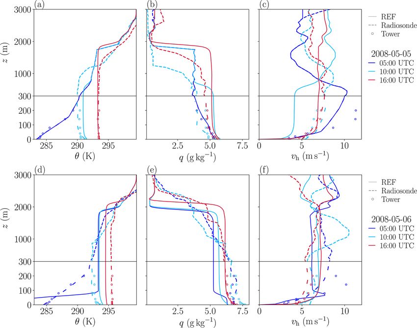
Figure 3 shows the time series of surface net radiation, which impact on the surface net radiation. The most obvious differ-
follows a diurnal cycle typical for clear-sky conditions. At ences occur in the albedo sensitivity simulations. An increase
noon, the reference simulation underestimates Rn , whereas
https://doi.org/10.5194/gmd-14-5307-2021 Geosci. Model Dev., 14, 5307–5329, 20215318 K. F. Gehrke et al.: Modeling of land–surface interactions in the PALM model system 6.0
in the albedo (case ALBE_24) decreases Rn and vice versa to −15 W m−2 , whereas the observations show a secondary
(case ALBE_04), with maximum deviation from case REF minimum of ca. −50 W m−2 between 20:00 and 23:00 UTC.
of approximately ±100 W m−2 at noon. This deviation sug- Here, we note that the depicted sensible heat fluxes from
gests that mismatches in the estimated albedo cause signifi- the simulations are domain-averaged values. Considered lo-
cant errors in the surface net radiation during daytime. How- cally in the simulation, we can detect similar temporal fluc-
ever, the spread of the non-highlighted simulations (gray) is tuations in H , though with a smaller amplitude than those
approximately 50 W m−2 at noon. This spread implies that observed at the CESAR site. The horizontal variation (max-
variations in the surface parameters (e.g., emissivity, rough- imum and minimum values) of the sensible heat flux of
ness length) also significantly affect the surface net radia- case REF is approximately ±30 W m−2 at noon. Like case
tion. Besides this, cases EMIS_95, EMIS_100, ROUGH_01, REF, all sensitivity simulations tend to overestimate the ob-
ROUGH_001, SOIL_2, and SOIL_4 are always among the served heat flux, and the spread among the considered cases
non-highlighted cases in Figs. 4, 5, and 6. With RRTMG, ra- is significant. At noon, when the spread among all simula-
diative fluxes are calculated for each horizontal grid box of tions is largest, differences in simulated heat fluxes approach
the LES based on time, geographical location, air pressure, 120 W m−2 . ALBE_24, LAI_3, and HUMID_dry show the
and local profiles of temperature and humidity (Clough et al., best agreement with the observations. With a higher albedo
2005) instead of being taken from measurements. A key fea- (ALBE_24), the available energy at the surface is lower (see
ture of the RRTMG is the direct cooling of air due to long- Fig. 3). The lower available surface energy results in smaller
wave radiative flux divergence, particularly during nighttime. fluxes of H and LE. Besides changing the albedo, cases
This results in cooling rates on the order of 0.1 to 0.3 K h−1 LAI_3 and LAI_05 show the largest impact on H because
(see, e.g., Maronga and Bosveld, 2017, their Fig. 1). This with lower and higher LAI the available energy is preferen-
effect is not included in case REF, wherein incoming radia- tially partitioned into H and LE, respectively. Similarly, the
tion is prescribed, and in case CLEARSKY. In case RRTMG, available energy is also preferentially partitioned into H and
the simulated Rn approaches that of the observations during LE for humid and dry air, indicated by HUMID_sat and HU-
day and night, though it slightly underestimates the surface MID_dry, respectively.
net radiation at noon by approximately 30 W m−2 . Note that
we use default input of the RRTMG with standard profiles
5.2.3 Latent heat flux
of water vapor, other trace gases, and aerosol concentration
above the model top, which does not necessarily reflect the
real conditions at Cabauw during the simulated time period Figure 5 shows time series of the latent heat flux. The ob-
and may impact the simulated surface net radiation as well. servations range from 0 W m−2 during the night to approx-
The clear-sky model simulates Rn more accurately during the imately 300 W m−2 at noon. Case REF matches the obser-
day but also marginally overestimates net radiation during vation reasonably well during daytime and nighttime, even
the night by 10 to 20 W m−2 . Case LAI_05 has a smaller Rn though it overestimates LE during the second day. The maxi-
than case REF because a smaller LAI significantly decreases mum and minimum values of latent heat flux for case REF in-
LE and increases H , which leads to higher surface temper- dicate low horizontal variation of approximately ±10 W m−2
atures during the day. Higher temperatures result in higher at noon. Having a lower LE than case REF, ALBE_24 best
LW↑ . In the case of a saturated humidity mixing ratio (case matches the observed LE of the second day. Additionally,
HUMID_sat), the surface temperature is higher during both case LAI_05 significantly underestimates LE by preferen-
day and night due to significant alterations to LE, H , and G. tially partitioning the available energy into H (Fig. 4). More-
This higher surface temperature again leads to higher LW↑ over, case HUMID_sat stands out because it shows a neg-
and hence lower Rn . Except for ALBE_04, the simulations ative LE during night due to dew formation in the model.
tend to underestimate the surface net radiation during day- Observations suggest that dew formation was not observed
time, while the simulated surface net radiation tends to over- in Cabauw because there is no negative LE. The maximum
estimate the observed surface net radiation during the night. spread of all non-highlighted sensitivity studies is approxi-
mately 50 W m−2 . This spread is up to 170 W m−2 for the
5.2.2 Sensible heat flux highlighted sensitivity studies. From Fig. 4 and Fig. 5 we
H
calculate the daytime Bowen ratio β0 = LE (not shown).
Figure 4 shows that the observed surface sensible heat We find that the difference between the Bowen ratio of the
flux reaches a maximum of approximately 100 and a mini- simulations and that observed at Cabauw (β0,sim − β0,obs )
mum of −50 W m−2 . Compared to observations (OBS), case ranges from −0.1 to +0.2, except for cases HUMID_sat and
REF significantly overestimates H by up to approximately LAI_05, which have significantly higher Bowen ratios com-
40 W m−2 , with the largest overestimation at noon. More- pared to observations. As opposed to other models, which
over, the model overestimates H in the morning and after- were shown to systematically overestimate the Bowen ratio
noon hours; it is positive earlier and later, respectively. At measured in Cabauw during summer (Schulz et al., 1998;
night, case REF shows a constantly increasing H from −25 Sheppard and Wild, 2002), we cannot identify a systematic
Geosci. Model Dev., 14, 5307–5329, 2021 https://doi.org/10.5194/gmd-14-5307-2021K. F. Gehrke et al.: Modeling of land–surface interactions in the PALM model system 6.0 5319
Figure 3. Time series of surface net radiation Rn as measured at Cabauw (OBS) and domain-averaged Rn for all simulated cases listed in
Table 5. Only case REF and some relevant cases are highlighted; all others are shown in gray. The gray transparent area shows minimum and
maximum values of the net radiation for case REF based on instantaneous hourly horizontal cross sections.
Figure 4. Time series of surface sensible heat flux H as measured at Cabauw (OBS) and domain-averaged H for all simulated cases listed
in Table 5. Only case REF and some relevant cases are highlighted; all others are shown in gray. The gray transparent area shows minimum
and maximum values of the sensible heat flux for case REF based on instantaneous hourly horizontal cross sections.
bias for the Bowen ratio of PALM’s LSM by means of the the temperature gradient between the surface and 0.5 cm is
analyzed period. accounted for. Hence, the simulated G resembles the diur-
Taking into account that modeled surface net radiation is nal cycle of the surface temperature, while the observed G
underestimated but the observed modeled latent and sensible correlates with the soil temperature. Observations and case
fluxes both exceed the observed values, while the modeled REF agree well at noon, with values of G around 55 W m−2 ,
Bowen ratio matches the observed values, one can conclude whereas in the afternoon at 15:00 UTC case REF is almost
that the remaining energy is included in the ground heat flux, 10 W m−2 higher than the observations. The horizontal vari-
which will be discussed in the next paragraph. ation (maximum and minimum values) of the ground heat
flux for case REF is approximately ±10 W m−2 at noon. Re-
5.2.4 Ground heat flux markably, all simulations have a fairly small spread at this
time. During the day, changing the heat conductivity between
Figure 6 shows the time series of the ground heat flux, the skin layer and uppermost soil layer has the largest im-
which reaches 60 W m−2 during daytime in the observations. pact on the ground heat flux, with smaller and larger G ob-
With respect to the amplitude of G, case REF shows good served in cases COND_2 and COND_6, respectively. This
agreement with the observation. However, the shape of the can be attributed to the linear relationship between G and 3
time series is discernibly different. During daytime, OBS has in Eq. (6). Also, the LAI sensitivity cases show a relatively
a pseudo-sinusoidal shape, whereas the simulations have a large deviation from case REF at noon, with increased (de-
more humped-shaped diurnal variation. We attribute this to creased) G for LAI_05 (LAI_3). At noon, the spread among
the method used to derive the observed ground heat flux, all simulations is approximately 40 W m−2 , whereas the non-
which involves the average soil heat flux at 10 and 5 cm highlighted cases show a maximum deviation from REF of
depths (details in Sect. 3). In the model, the ground heat no more than ±10 W m−2 . In the night, cases HUMID_sat
flux is parameterized according to Eq. (6), and thus only
https://doi.org/10.5194/gmd-14-5307-2021 Geosci. Model Dev., 14, 5307–5329, 2021You can also read