Morphological classification of galaxies with deep learning: comparing 3-way and 4-way CNNs

MNRAS 000, 1–18 (2021) Preprint 4 June 2021 Compiled using MNRAS LATEX style file v3.0

 Morphological classification of galaxies with deep learning:
 comparing 3-way and 4-way CNNs

 Mitchell K. Cavanagh,1★ Kenji Bekki1 and Brent A. Groves1,2
 1 ICRAR M468, The University of Western Australia, 35 Stirling Hwy, Crawley, WA 6009, Australia,
 2 Research School of Astronomy and Astrophysics (RSAA), Australian National University, ACT 2611, Australia

 Accepted XXX. Received YYY; in original form ZZZ
arXiv:2106.01571v1 [astro-ph.GA] 3 Jun 2021

 ABSTRACT
 Classifying the morphologies of galaxies is an important step in understanding their physical
 properties and evolutionary histories. The advent of large-scale surveys has hastened the need
 to develop techniques for automated morphological classification. We train and test several
 convolutional neural network architectures to classify the morphologies of galaxies in both
 a 3-class (elliptical, lenticular, spiral) and 4-class (+irregular/miscellaneous) schema with a
 dataset of 14034 visually-classified SDSS images. We develop a new CNN architecture that
 outperforms existing models in both 3 and 4-way classification, with overall classification
 accuracies of 83% and 81% respectively. We also compare the accuracies of 2-way / binary
 classifications between all four classes, showing that ellipticals and spirals are most easily
 distinguished (>98% accuracy), while spirals and irregulars are hardest to differentiate (78%
 accuracy). Through an analysis of all classified samples, we find tentative evidence that mis-
 classifications are physically meaningful, with lenticulars misclassified as ellipticals tending
 to be more massive, among other trends. We further combine our binary CNN classifiers
 to perform a hierarchical classification of samples, obtaining comparable accuracies (81%)
 to the direct 3-class CNN, but considerably worse accuracies in the 4-way case (65%). As
 an additional verification, we apply our networks to a small sample of Galaxy Zoo images,
 obtaining accuracies of 92%, 82% and 77% for the binary, 3-way and 4-way classifications
 respectively.
 Key words: galaxies: general – methods: miscellaneous

 1 INTRODUCTION human classifiers, while the speed of the actual classification itself
 is more or less unchanged. Future large-scale surveys are expected
 Galaxies exhibit a variety of morphologies throughout cosmic time
 to yield enormous amounts of data, with Euclid alone expected to
 (Conselice 2014), ranging from broad families of spirals to large
 survey at least to the order of 1 billion galaxies. The scale of sur-
 ellipticals. A galaxy’s morphology is related to its internal physical
 veys such as these will overwhelm the capacity of human volunteers
 processes (Sellwood 2014), such as its dynamical and chemical
 (Silva et al. 2018), necessitating the development and deployment
 evolution, star formation activity (Kennicutt 1998), and can reveal
 of techniques for automated classification.
 insights into its past evolutionary history, including mergers (Mihos
 & Hernquist 1996) and interactions with its environment (Alonso Automated classification techniques, in particular those util-
 et al. 2006). A galaxy’s morphology is often determined by visual ising neural networks (Dieleman et al. 2015; Domínguez Sánchez
 inspection, and while this is sufficient to delineate a rich array of et al. 2018; Zhu et al. 2019), have the ability to revolutionise the
 morphological types in the nearby Universe (Buta 2013), there is speed at which samples can be individually classified. Such clas-
 the inherent issue of scalability as future surveys yield far greater sification techniques range from analytical approaches, such as the
 magnitudes of data. Fourier analysis of luminosity profiles (Odewahn et al. 2002) and
 Visually classifying the apparent morphologies of galaxies isophote decompositions (Méndez-Abreu et al. 2017), to statistical
 through the manual inspection of images is a laborious, time- learning methods (Sreejith et al. 2017), random forest classifiers
 consuming task. Recently, the use of citizen science has seen great (Beck et al. 2018) and ensemble classifiers (Baqui et al. 2021),
 success in classifying larger datasets (Lintott et al. 2011; Willett which are all part of a broader suite of machine learning methods
 et al. 2013; Simmons et al. 2016), however it is important to keep in (Cheng et al. 2020). Neural networks have been utilised in this field
 mind that this was achieved by increasing the order of magnitude of for some time, but only recently has the rapidly growing field of deep
 learning seen widespread applications in astronomy (Baron 2019).
 One of the key architectures behind the success of deep learning,
 ★ E-mail: mitchell.cavanagh@icrar.org (MKC) particularly in applications involving image recognition and com-

 © 2021 The Authors

2 M. K. Cavanagh et al.
puter vision, is the convolutional neural network (hereafter CNN), whether by eye or by CNN. As a final, independent verification of
introduced by Lecun et al. (1998). Unlike the typical multiplayer per- our network, we apply our models to a small sample consisting of
ceptrons present in a normal neural network, CNNs are specifically 1,000 randomly chosen ellipticals and 1,000 randomly chosen spi-
designed to extract features in data through multiple convolutions ral galaxies from the Galaxy Zoo dataset. Lastly, we summarise our
(LeCun et al. 2015). Each convolution can be thought of as a layer findings in §5.
of abstraction, with the extracted high-level features used to learn
a generalised representation of data. Importantly, CNNs provide a
model-independent means of feature extraction, hence their versatile 2 METHODS
range of applications. Although having originally been developed
to recognise handwritten characters, modern CNNs are capable of 2.1 Dataset
general image recognition across myriad image types (He et al. The Nair & Abraham (2010) catalogue, hereafter NA10, contains
2015). Indeed, image classification is one of the main astronomical 14,304 visually classified samples from the SDSS Data Release 4
applications of CNNs (Cheng et al. 2020). (Adelman-McCarthy et al. 2006). These are all single-band, g-band
 CNNs have been successfully utilised to detect quasars and images with spatial resolutions of 50 kpc. Of key interest to this work
gravitational lenses (Pasquet-Itam & Pasquet 2018; Schaefer et al. are the Hubble T-Type classifications, which range from -5 to 12
2018), study bulge/disk dominance (Ghosh et al. 2020), detect stellar with a miscellaneous 99 category for samples with no clear category.
bars (Abraham et al. 2018) and classify radio morphologies (Wu The miscellaneous category also includes interacting galaxies and
et al. 2018). CNNs have also been widely used with simulations, mergers. One of the goals of the catalogue is to serve as a dataset
including cosmological simulations (Mustafa et al. 2019) and mock with which to calibrate automated classification techniques.
surveys (Ntampaka et al. 2020), as well as to develop tools for galaxy For this work, we consider up to four morphological categories;
photometric profile analysis (Tuccillo et al. 2017). Recent studies ellipticals (E), lenticulars (S0), spirals (Sp) and irregulars plus mis-
have utilised CNNs for the purpose of binary classification (Ghosh cellaneous types (Irr+Misc). The samples in the Nair catalogue have
et al. 2020), or classifying between general morphological shapes T-Types that range from -5 to 12, with a miscellaneous T-Type 99.
(Zhu et al. 2019). Fewer studies have looked at 3-way classification Table 1 outlines our definition of the four morphological classes,
between distinct morphological types, though some works have along with the NA10 T-Types and the classic RC3 (de Vaucouleurs
explored classifying between ellipticals and barred/unbarred spirals et al. 1991) schema for reference. Using these definitions, 2723
(Barchi et al. 2020), or between ellipticals, spirals and irregulars samples are categorised as ellipticals, 3215 as S0s, 7708 as Spirals
(Calleja & Fuentes 2004) and 388 as Irr+Misc.
 In this work, we train and test several different CNN architec-
tures for the purpose of initially distinguishing between elliptical
(E), lenticular (S0) and spiral (Sp) galaxies, before extending the 2.2 Convolutional Neural Networks
schema to include a fourth irregular and miscellaneous category In this section we briefly outline the theory of neural networks,
(Irr+Misc). We base our training data on the visually classified cata- introduce some key terminology and explore how CNNs differ from
logue of Nair & Abraham (2010), consisting of 14034 samples from standard neural networks. A standard, fully-connected, feed-forward
the SDSS Data Release 4 (Adelman-McCarthy et al. 2006), and ap- artificial neural network consists of multiple layers of nodes, such
ply a series of data augmentation techniques to increase the number that each node is connected to all the nodes in its preceding and
of training samples for use with the CNN. Our best accuracies are succeeding layers (Haykin 2009; Goodfellow et al. 2016). The input
consistent with previous studies, surpassing others when it comes data is mapped to the nodes in the input layer, with the nodes in the
to per-class accuracies. We dedicate a section of our discussion to final layer corresponding to the outputs. Each node has an activation
focusing on the physical implications of the CNN classifications value that is obtained as follows:
(both correct and incorrect), as well as how these are reflective of
 −1
the inherent uncertainty in the training data, how such uncertainties © ∑︁ −1 
 = ­ , + ®
 ª
affect CNN accuracies, and how CNNs can be used to address these
uncertainties. « ¬
 The structure of the paper is as follows. In §2 we briefly outline where denotes the current layer, denotes the current node, −1
the theory of CNNs and its key concepts and terminology, discuss is the number of nodes in the previous layer, −1
 is the activation of
the CNN architectures including our new C2 network, discuss the
augmentation and training methodology, and discuss the overall the th node in the previous layer, , is the weight assigned to the
performance of the 3-way and 4-way classification tasks for each edge connecting the current node to the previous node −1 
 , 
of the four CNN architectures. In §3 we present our key results, is a bias, and is an activation function. To train a neural network,
starting with binary classifications between morphological classes, we supply it with at least two similarly representative sets of data;
before presenting the best results for the 3-way and 4-way classifi- a training set, and a test set. A third validation set, independent of
cations and analysing these by considering the physical properties the test set, is used to tune the hyperparameters of the network. The
of the samples for each classification. In §4 we discuss the accu- neural network is trained by adjusting the weights and biases
racy of the CNN. We examine the physical properties of classified for all nodes in every layer to minimise the error (with respect
samples and show that there are common trends in the misclassified to an objective or loss function) with the desired outputs in the
samples across several physical properties. We showcase binary hi- training set. This is usually achieved via a learning algorithm such
erarchical classification as an alternative to the direct multi-class as gradient descent over multiple iterations of training, where each
CNNs, exploring five different classifiers and their key differences iteration is referred to as an epoch. Once trained over a sufficiently
to our main CNN. We present several examples of images that were large number of epochs, the final success rate is determined via an
correctly and incorrectly classified, commenting on inherent uncer- evaluation on an unseen test set. The training is typically conducted
tainties and the challenge of unambiguously classifying samples, in batches, with the weights and biases updated for each batch.

 MNRAS 000, 1–18 (2021)

Morphological classification of galaxies 3

Table 1. Definition of our four morphological categories in terms of Hubble morphologies and numerical T-Types schemas. Ellipticals are defined as c0 to E+
(Nair T-Type -5 only), S0s defined as S0- to S0/a (Nair T-Types -3 to 0), Spirals as Sa to Sm (Nair T-Types 1 to 9), and Irr+Misc as Im onwards (Nair T-Types
10 and 99).

 Category Elliptical S0 Spiral Irr+Misc

 Class c0 E0 E+ S0- S0 S0+ S0/a Sa Sab Sb Sbc Sc Scd Sd Sdm Sm Im Misc
 RC3 -6 -5 -4 -3 -2 -1 0 1 2 3 4 5 6 7 8 9 10 -
 Nair -5 -5 -5 -3 -2 -2 0 1 2 3 4 5 6 7 8 9 10 99

 CNNs are a specialised type of neural network designed to 2.3 Model Architectures
extract high-level features from the provided input data through the
application of convolutions. Each 2D convolutional layer takes an In this work we consider four principal CNN architectures, each
 × input array and applies filters/weights using a × kernel with different complexity and originally designed for different input
(a.k.a window), where < , in order to obtain unique feature image sizes. All architectures are designed to accept single-band
maps. In particular, if the input to a convolutional layer is a set of images as their input. Figure 1 displays a schematic illustration of
 for = 1, . . . , , then the feature maps are given as
matrices X −1 each architecture. Each architecture is built using Keras (Chollet
 et al. 2015), a high-level machine learning interface. The first CNN,
 referred to as C1, is based on our previous work (Cavanagh & Bekki
 2020), and was originally designed for the binary classification of
 
 !
 ( ) ( , ) ( ) ( )
 ∑︁
X = W ∗ X −1 + 50 × 50 imagery. This architecture consists of a single block of
 =1 convolution and pooling layers (2 Conv2D plus a MaxPooling), a
 penultimate Dense layer with 256 nodes, and the output Dense layer
 ( , ) which contains either 3 or 4 nodes for 3-way or 4-way classification.
where denotes the th feature map, W are the filters/weights
 The second CNN architecture is based on the work of Diele-
 ( )
for layer , input map and feature map , is a vector of biases, man et al. (2015). This architecture contains multiple convolutional
and is a (multi-dimensional) activation function. Here ∗ denotes blocks, starting with two blocks of alternating, single Conv2D and
a linear convolution. Note that the inputs and feature maps need not MaxPool layers, then a block of two successive Conv2D layers fol-
be square. Importantly, each feature map is convolved from the input lowed by a final MaxPool. There are also two Dense layers before
 ( , )
image with a different set of filters/weights. These weights W the output layer. Key differences to the original implementation in
are learnable and are tweaked during training. Key to the success Dieleman et al. (2015) is that we make use of the Adadelta adaptive
of CNNs is that they learn multiple filters in parallel, which enables learning rate algorithm for training (Zeiler 2012), and we have also
the network to not only obtain different abstract representations of added Batch Normalisation layers at the end of every convolutional
the data, but also use these in order to distinguish between data of block. When training a network, the training data is usually pro-
different types. cessed in batches, with the weights and biases tweaked after each
 Unlike in a normal neural network, where each node’s edges batch. Batch normalisation is used to enforce uniformity across all
are free parameters, feature maps use shared weights by apply- samples in a batch by keeping a consistent mean and standard devi-
ing a single convolutional filter across the entire input, rather than ation. This has the effect of smoothing the objective function (hence
separate filters for individual parts of the input. Thus, in order to smoother gradients), leading to better performance, improved regu-
minimise the loss with the training data, the CNN directly adjusts larisation and generalisation (Ioffe & Szegedy 2015; Santurkar et al.
these filter weights, hence obtaining different feature maps. As such, 2019).
CNNs provide a model independent means to classify images, re- The third architecture is based on AlexNet (Krizhevsky et al.
lying solely on self-taught convolution weights to extract the most 2012), a network designed for general image classification. This
meaningful features in data. Successive convolutional layers are architceture has commonly been used in many classification prob-
used to extract higher-level features. Generally, later convolutional lems, including most recently in astronomy (Ghosh et al. 2020).
layers extract more feature maps with smaller kernels. This is the most complex architecture out of the four, and is notable
 CNNs also contain another important layer known as a pool- for its heavy use of dropout regularisation with two Droput layers,
ing layer. These layers are used to down sample feature maps (Zhou each dropping 50% of the previous layer’s nodes. The convolutional
et al. 2015). For this work, we use MaxPooling. This method of layers also utilise a large number of filters. The original optimiser
pooling preserves the maximal elements, helping to highlight dom- used for the training of this network is stochastic gradient descent
inant features. This also helps to introduce a degree of translational with momentum, however the learning rate is computationally ex-
invariance and also serves to reduce noise. After the features have pensive to tune. Instead we use the Adadelta adaptive learning rate
been extracted via convolutional and pooling layers, all the feature algorithm. We also add batch normalisation layers after each con-
maps are flattened into a single 1D array. These are then fully con- volutional block but before the max pooling, adding even more
nected to subsequent layers of nodes (referred to as Dense layers), regularisation to the network.
ultimately ending with the output layer which contains a total num- The fourth architecture, named C2, is completely new from this
ber of nodes equal to the total number of output categories. These work, designed as a three-block CNN with two dense layers, a single
layers are functionally identical to a normal neural network. After dropout layer, and batch normalisation throughout. Unlike previous
flattening the feature maps, it is common to remove a fraction of models, we decided to use the Adam (Adaptive Moment Estimation)
randomly selected nodes. This is an efficient regularisation tech- algorithm (Kingma & Ba 2014), an efficient stochastic gradient
nique known as Dropout, and is used to reduce overfitting of the descent algorithm that can be considered an extension of Adadelta.
data and improve generalisation (Srivastava et al. 2014). Unlike Adadelta, Adam’s learning rate must be pre-specified. To

MNRAS 000, 1–18 (2021)

4 M. K. Cavanagh et al.

Figure 1. Schematic representation of all four principal CNN architectures used in this work: the CNN from Cavanagh & Bekki (2020) (C1), the CNN based
on Dieleman et al. (2015) (Diel), the CNN based on Krizhevsky et al. (2012) (Alex), and our new CNN introduced in this work (C2). Layers are colour coded:
grey for convolutional layers, red for pooling, light blue for dropout and blue for dense layers. Convolutional layers are annotated with the number of feature
maps, followed by the kernel size. Pooling layers are annotated with the size of the pooling. Dropout layers are annotated with the dropout rate (the fraction of
nodes ignored in the previous layer). Dense layers are annotated with the number of nodes.

 MNRAS 000, 1–18 (2021)

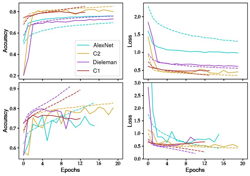
Morphological classification of galaxies 5
determine the optimal design for our C2 architecture, including cropping is a case of diminishing returns given the lack of any
the best learning rate, we performed hyperparameter tuning with meaningful improvement to the overall accuracy.
the tool Keras Tuner (O’Malley et al. 2019). A hyperparameter In this study, our primary resolution for the input image data
is any value that affects the architecture of a neural network (e.g. is 100 × 100. We also perform some further runs at 200 × 200 to
number of nodes) or the manner in which it is trained (e.g. learning assess the impact of changing resolution, however it is important
rate). Hyperparameter tuning refers to the process of optimising the to note that the prohibitively expensive memory and computational
hyperparameters within the search space as specified by the range of requirements for the 200×200 runs restricted the degree of augmen-
desired values. In the case of C2, we started with the same sequence tation (in particular, no cropping). This is since the limited amount
of layers in Figure 1, and used hyperparameter tuning to determine of GPU memory available necessarily places an upper limit on the
the optimal number of feature maps for each convolutional layer (out total number of samples that can be trained with at a given reso-
of a choice of 32 or 64 for the first convolutional layer, and 64 or 128 lution. Instead, we direct most of our focus to the fully augmented
for all layers thereafter), width of the convolutional filter or kernel 100 × 100 data. The original imagery in the NA10 dataset comes
(7x7 or 5x5 for the first layer, 5x5 or 3x3 for all others), number in variable resolutions, the most common of which were between
of nodes in the dense layers (256, 512 or 1024), degree of dropout 100 and 130 pixels. These were all resized to the desired, target res-
(0.3, 0.4 or 0.5), whether to use max pooling or average pooling, and olution using cubic interpolation with Pillow, a fork of the Python
finally the learning rate for the Adam optimiser, to be determined Imaging Data. The raw pixel data was extracted and reshaped into
by sampling between 10−3 and 10−4 . The optimal parameters for the correct format for loading into the CNN. All input images were
the C2 architecture, as determined by hyperparameter tuning, are linearly normalised such that pixel values are between 0 and 1. No
annotated in Figure 1. The final, tuned learning rate for the Adam further alterations were made to the images.
optimiser was 2 × 10−4 .
 Across all architectures, we used consistent activation func-
tions, with ReLU for all convolutional and dense layers, and with 2.5 Training and Validation
a final softmax activation for the output layer. Softmax, a type of The CNNs were constructed with the high-level API Keras (Chol-
normalised exponential, is important as it converts the activations let et al. 2015) and trained using the TensorFlow machine learning
into probabilities that sum to 1 across all output categories. The pre- library running with nVidia’s GPU programming toolkit CUDA.
dicted category, or simply the prediction, is just the category with Training was conducted on ICRAR’s Hyades cluster, making use
the maximum value (in other words, the output node with the high- of a Nvidia GTX 1080 Ti graphics card, with smaller-scale runs
est activation). This maximum value itself is often referred to as the and testing performed on a Nvidia GTX 1650 Ti laptop graphics
probability or confidence; we will use both terms interchangeably. card. The dataset was first partitioned into separate training and test
 sets according to an 85:15 split, i.e. 15% of the dataset is reserved
 for testing, with 85% used for training. The training set was further
2.4 Data Augmentation and Pre-Processing partitioned into separate training and validation sets (again with an
 85:15 split) for the purpose of hyperparameter tuning. A third val-
The size of the NA10 dataset is relatively small given the complex- idation set, fully independent of the actual test set, is necessary for
ity of the CNN architectures, and is thus prone to overfitting. In hyperparameter tuning in order to avoid biasing the choice of hy-
order to increase the size of the dataset, and subsequently improve perparameters. Thus, when the optimal network is finally trained, it
the performance of the CNN, we apply several data augmentation is evaluated on an independent, unseen dataset. This is an important
techniques. These are listed as follows: test of the network’s ability to effectively generalise.
 • Cropping. For an image of size × we can crop multiple Training was conducted over a maximum of 100 epochs with
 × images for > . We have chosen to crop each image from a batch size of 400 for 100 × 100 data, and a reduced batch size of
each corner, as well as in the center, for a total of five cropped 200 for the 200 × 200 data due to memory limitations. To conduct
images. Cropping was done with an 110 × 110 image to yield five these runs efficiently, we used early stopping; a method of ceasing
100 × 100 images. training once there is no appreciable improvement in the validation
 • Rotation. We rotate each image by 90◦ increments, yielding loss over a threshold number of epochs. This threshold - the number
four images. of epochs over which to monitor whether the training is improving
 • Flipping / Mirroring. Yields two new images. Our implemen- or not - is known as the patience. All runs were conducted with a
tation is equivalent to a flip about the axis = . patience of 7, and had generally converged and been stopped by the
 20th to 25th epoch. Early stopping helps to avoid wasting unnec-
As implemented, these techniques combine to increase the number essary computations once the validation accuracy has plateaued,
of images by a factor of 40, from 14,034 to a maximum of 561,360 and subsequently prevents overfitting. The best weights were stored
images. An example of these techniques as applied to a sample using Keras’ ModelCheckpoint callback function. We make use of
spiral galaxy from our training set is shown in Figure 2. These the categorical cross-entropy loss function for all CNNs.
data augmentation techniques also help to generalise the input data Figure 3 shows all training and final validation accuracies/loss
and enforce a degree of spatial and translational invariance. This is for all four CNN architectures. Note here that the validation accu-
important, as the CNN must learn to identify the features themselves, racy/loss is merely a metric based on evaluations on the test set. All
and not simply that they are present in specific regions within the the weights and biases are initially randomised at the start of train-
feature maps. Based on preliminary experiments with a small subset ing. It can be seen that the validation accuracies initially rise rapidly
of the total data, we found that both rotating and flipping had a before plateauing. Similarly, the validation loss gradually falls be-
noticeable, positive impact on the overall training accuracy, albeit fore becoming constant; indeed, early stopping is used to halt the
similar effects due to cropping were not as pronounced. We chose training when the loss no longer decreases. Were early stopping not
only to process five cropped images to maintain a reasonable file employed, the validation loss would continue to increase (see the
size while keeping within our computational limitations; any further C1 and AlexNet 4-way plots in the bottom-right panel of Figure

MNRAS 000, 1–18 (2021)

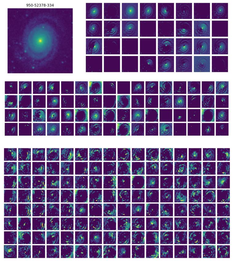
6 M. K. Cavanagh et al.

Figure 2. An example of our principal data augmentation techniques (cropping, mirroring and rotating) as applied to a spiral galaxy. The original image is on
the left.

Figure 3. Accuracies and loss for all four CNN architectures for the 3-way (top panels) and 4-way (bottom panels) classification schemas as functions of the
number of epochs, and as trained on the 100 × 100 data. The training accuracy/loss is represented with a dotted line, while the validation accuracy/loss is
represented with a solid line. Architectures are represented with C1 in red, C2 in yellow, AlexNet in cyan and Dieleman in magenta.

3), further widening the gap with the training loss and resulting tional and pooling layers in order to understand how the network
in overfitting. The accuracy and loss values exhibit large random is interpreting the input data; in particular, the features that are be-
fluctuations, especially in the 4-way case, which is another sign of ing extracted via the learnable filter weights. Figure 4 shows every
overfitting. As can be seen in Figure 3, our C2 network is the best individual feature map in the first, third and fourth convolutional
overall performer, since it is less affected by overfitting and achieves layers of the C2 CNN architecture (see Figure 1) for the shown
lower overall validation losses compared to the other models. Note spiral galaxy in the 3-way case. It can be seen that, after more and
the validation accuracy and loss are purely metrics corresponding more convolutions and poolings, the features maps become more
to repeated evaluations of the network with the independent test set abstract. Through the use of these convolutions, the CNN is able to
at the conclusion of every epoch. In Keras, these steps do not affect extract relevant features from the input image, such as spiral arms,
any of the network parameters. the central bulge, and even a trace of the outline of the galaxy itself.
 It is important to stress that the filters/weights for each convolution
 It is useful to visualise the feature maps within the convolu-

 MNRAS 000, 1–18 (2021)

Morphological classification of galaxies 7
are initially random and have instead been learned by the network. Table 2. Best classification accuracies of the principal CNN architectures
Thus visualising the feature maps enables us to see the results of for different input sizes and number of output categories, with 3-way distin-
these convolutions, and in the case of Figure 4, the images that the guishing between E, S0 and Sp, and 4-way distinguishing between E, S0,
CNN has learned to interpret as a spiral galaxy. Sp and Irr+Misc.

 Network Input Size Best 3-Way Best 4-Way

3 RESULTS C1 100 × 100 79% 75%

3.1 Binary classifications Dieleman 100 × 100 82% 76%

Before classifying galaxies as either ellipticals, lenticulars, spirals 200 × 200 82% 79%
or irregulars/misc, it is useful to first consider binary classifications AlexNet 100 × 100 75% 74%
between all four of these classes. This allows us to anticipate which
distinctions are most problematic and likely to be sources of confu- 200 × 200 84% 83%
sion. This will further serve to assist in interpreting the confusion C2 100 × 100 83% 81%
matrices of the 3-way and 4-way classification.
 We conducted two-way classifications between all four mor- 200 × 200 81% 80%
phological classes (E vs S0, E vs Sp, . . .) using our newly developed
C2 network architecture. We further conducted two-way classifica-
 Increasing the resolution to 200 × 200 has a marginal effect on the
tions between combinations of classes: Sp vs E and S0 (this can be
 overall classification accuracies, with only the AlexNet architecture
considered an early vs. late type classifier), E vs. S0 and Sp, and ir-
 producing a consistent gain. Given the resultant four-fold increase
regulars vs. regulars, where regulars are subsampled from all E, S0
 in computationally complexity and memory requirements for little
and Sp samples. Since there are an extremely low number irregulars
 comparative gain, we instead base our analysis on the 100 × 100
in the training set compared to the other classes, the 2-way classifi-
 data. Our achieved accuracies are comparable to recent CNN appli-
cations involving irregulars used a training set with an equal number
 cations, e.g. Barchi et al. (2020) with 83% for 3-class classification
of samples from each class, hence the over-represented class was
 (albeit for ellipticals and barred/unbarred spirals).
randomly subsampled. In these cases, the performance is dependent
 Accuracy alone is not sufficient to judge the overall perfor-
on the quality of the subsample (insofar as its resemblance, or lack
 mance of a CNN. When it comes to multi-class classification, it is
thereof, to the full sample), so each run was repeated multiple times
 necessary to consider how the classifications are distributed. The
with different subsamples, with the mean accuracy taken as the final
 confusion matrix is one way of comparing the true or correct labels
result. The “regulars” training set used for the irregular vs. regular
 to the predicted labels. As is conventional for machine learning,
run was created with an equal number of samples from the E, S0
 rows correspond to the actual, true classes, while columns corre-
and Sp categories. All other runs not involving irregulars (e.g. E vs
 spond to the predicted classes (i.e. the label returned by the neural
Sp) were conducted with all the available data, hence needing only
 network). With this convention, the cell (E, S0) refers to true ellip-
a single run. All datasets were partitioned according to an 85:15
 ticals classified by the network as lenticulars. The confusion matrix
split into training and testing sets.
 of a perfectly accurate CNN is an identity matrix.
 Figure 5 shows the classification accuracies for all the afore-
 Figures 6 and 7 show confusion matrices for both the 3-way
mentioned binary classifications. Ellipticals and spirals are able to
 and 4-way classifications respectively, using the best-performing
be distinguished with a very high accuracy (>98%), spirals and
 C2 neural network architecture, and trained on 100 × 100 resolution
lenticulars at 88%, ellipticals and irregulars at 86%, spirals and
 images. In the case of the 3-way classification, spirals are most
irregulars at 79%, ellipticals and lencitulars at 78%, and lastly
 accurately classified (93%), following by ellipticals (80%) and S0
lenticulars and irregulars at 70%. We also find that spirals can
 (60%). S0s are almost equally misclassified as E or Sp (18% and
be disassociated from Es and S0s combined with a high accuracy
 22% respectively). Almost all the misclassified E were misclassified
(91%); similarly for Es vs. S0s and spirals (92%). Lastly, irregulars
 as S0, with just 1% misclassified as spirals. Similarly, just 6% of true
vs. regulars had an accuracy of 84%, although it is important to
 spirals were misclassified as S0. Thus it is clear that ellipticals and
keep in mind that this used a considerably smaller training set as
 spirals are the easiest morphological classes to distinguish between,
there were so few irregulars. These results are consistent with ex-
 while S0s are considerably more difficult.
pectations from previous, established studies, e.g. Calleja & Fuentes
 In the 4-way classification case (Figure 7), we find that both el-
(2004) obtained a 95% accuracy for E vs Sp.
 lipticals and spirals have strong prediction accuracies (87% and 89%
 respectively). The accuracy of classifying S0s is unchanged, while
 the fourth irregular/miscellaneous class has a very poor accuracy
3.2 3-way and 4-way classifications
 only slightly higher than random. It is likely that the low accuracy
Many previous studies utilising CNNs in astronomy have used bi- of the irregular class is a contributing factor to the accuracy and
nary classifications. In this study, we directly train a CNN to clas- loss fluctuations in Figure 3. The majority of irregular samples are
sify firstly between three classes, and again between four. Table 2 misclassified as spirals (50%) or S0s (21%). This is likely due to a
presents a summary of the overall classification accuracies for all combination of low-population categorical bias (there are only 388
CNN architectures with both 100 × 100 and 200 × 200 data. Note irregular/misc samples out of 14034 total samples), and the fact that
that memory limitations prevented the C1 architecture being used many miscellaneous samples show evidence of mergers, interaction
with the 200 × 200 data. Our C2 architecture outperforms all other and/or fine structure that may be interpreted as spiral or S0-like.
models with the 100 × 100 data, with only the 200 × 200 4-way This will be further analysed and discussed in Section §4, where we
AlexNet run beating it. We obtain accuracies of 83% and 81% for discuss hierarchical classification.
3-way and 4-way classifications respectively with 100 × 100 data. Another means of assessing the performance of CNNs is to

MNRAS 000, 1–18 (2021)

8 M. K. Cavanagh et al.

Figure 4. Plot of each individual feature map in the first, third and final convolutional layers of the C2 network, as generated for the example spiral galaxy
shown in the top-left.

consider the overall F1-scores for each category. The F1-score is icative value or PPV. Recall is defined as
the harmonic mean of the precision and recall. In the context of TP
machine learning, the precision of a neural network is defined as Recall =
 TP + FN
 TP where FN denotes false negatives. It is equivalent to the sensitivity
Precision = or true positive rate, as it measures the fraction of correctly identified
 TP + FP
 positives. The F1-score is thus simply
where TP and FP denote true positives and false positives respec- Precision × Recall
tively. Precision, in this context, is equivalent to the positive pred- F1 = 2 ×
 Precision + Recall

 MNRAS 000, 1–18 (2021)

Morphological classification of galaxies 9

Figure 5. Binary classification accuracies for various combinations of morphological types as trained and tested with the C2 network. Accuracies are coloured
according to relative accuracy, with dark green corresponding to the strongest distinction (E vs. Sp at 98%) and olive corresponding to the weakest distinction
(Sp vs. Irr+Misc at 78%).

 Table 3. Precision, recall and F1 scores for the best 3-way and 4-way
 classifications with our C2 network

 Class Precision Recall F1-Score

 E 0.79 0.80 0.79
 S0 0.65 0.60 0.62
 Sp 0.91 0.93 0.92

 Weighted Avg 0.82 0.83 0.83

 E 0.75 0.87 0.81
 S0 0.61 0.60 0.60
 Sp 0.91 0.89 0.90
 Irr+M 0.48 0.27 0.35

 Weighted Avg 0.80 0.80 0.80

Figure 6. The confusion matrix of our C2 network for the 3-way classi-
fication between ellipticals (E), lenticulars (S0) and spirals (Sp), coloured
according to the accuracy of the classification.

 Figure 8. Distribution of the confidences for each classified sample for both
 the 3-way (blue) and 4-way (purple) CNNs

 and has a value between 0 and 1. The higher the F1-score, the better.
 Tables 3 shows the precision, recall and F1-scores for our 3-way and
 4-way classifications respectively. In general, spirals and ellipticals
Figure 7. The confusion matrix of our C2 network for the 4-way classifica- perform best. Although the precision is quite high for the irregu-
tion between ellipticals (E), lenticulars (S0), spirals (Sp) and irregular/misc lar/miscellaneous samples, the recall is only slightly higher than
samples (Irr), coloured according to the accuracy of the classification. random. This is indicative of the challenge in accurately classifying
 low populations of irregulars.
 It is also useful to analyse the distribution of the confidence of

MNRAS 000, 1–18 (2021)

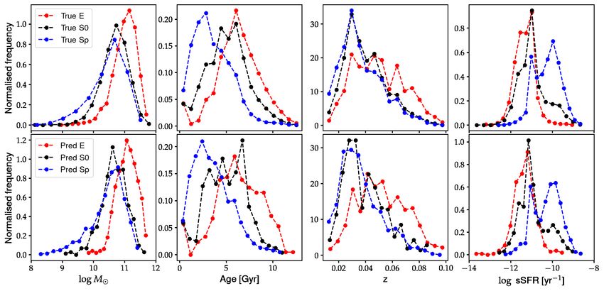
10 M. K. Cavanagh et al.
each sample; that is, the probability that it belongs to the predicted confusion matrices” are shown in Figure 9 where we are calcu-
class. As we have used a softmax activation function for the output lating the median age, redshift and stellar mass for each sample
layer, the activation values all sum to 1 across all categories. The based on their classification, e.g. median age of all true ellipticals
predicted class is simply the category with the largest probability, classified as E, S0, Sp, all true spirals classified as E, S0, Sp, etc.
and the value of that largest probability is known as the confidence. All values are from the NA10 tables, with the values for physical
Figure 8 shows the distribution of these confidences for all samples quantities based on the MPA/JHU catalogues. As expected, true el-
in both the 3-way and 4-way classifications. Most samples are clas- lipticals have higher redshifts, masses and are older than their spiral
sified with a high degree of confidence, however the fact that the counterparts. While this is expected given the general pathway of
distribution is smooth at high to mid probabilities indicates that the morphological evolution (Conselice 2014), this is also reflective of
CNN has not been unduly overfitted. In a highly overfitted CNN, the sample biases at higher redshifts where bright, compact objects
the confidences would all cluster around 1 with little to no tail. like elliptical galaxies are more easily detected.
 Given the values for the confused samples, there is evidence
 that even the misclassifications are physically meaningful. In the
 case of redshift, true ellipticals misclassified as S0s have (1) a lower
4 DISCUSSION
 median redshift than correctly classified ellipticals, and (2) a higher
4.1 Classification Accuracies median redshift than correctly classified true S0s. Similarly, the me-
 dian redshift is higher for both true S0s classified as ellipticals and
In general, our binary classification accuracies (Figure 5) are com- true spirals classified as ellipticals. These trends are also observed
parable to those of other studies. Our accuracy of 98% for ellipticals for the other two properties: true ellipticals misclassified as S0 are
vs. spirals is in line with other studies (Domínguez Sánchez et al. less massive and younger than correctly classified true ellipticals,
2018; Barchi et al. 2020), and also compares well with other early and are also more massive and older than correctly classified true
vs. late-type classifiers (de Diego et al. 2020). The key issue when it S0s. These trends are also seen in the 4-way physical confusion ma-
comes to training a binary classifier CNN is that there are an unequal trices for all but the irregular class, where the low number of samples
number of samples for each class. This is most prominent with the makes it difficult to establish any trends. Note that empty cells in
irregular/miscellaneous samples, a mere 2.8% of the total sample. some of the four-way confusion matrices are where no physical data
With such a disparity, it is necessary to choose a subset of the over- is available for the sample(s) present. Importantly, the S0 and spiral
represented category in order to equalise the number of samples in samples misclassified as ellipticals are more distant, more massive
each category, and hence reduce categorical bias. However, given and older than true S0s and spirals. Each of these characteristics are
the smaller overall dataset, there is a higher risk of overfitting, which indeed to be expected of an elliptical galaxy. Thus this demonstrates
the data augmentation is able to partially ameliorate. that the CNN has learned to identify features that discriminate be-
 Our best, direct 3-way classification accuracy of 84% is also tween the different morphological types. If the misclassifications
consistent with recent studies (Barchi et al. 2020), thought we note were random then we would not see such a trend across multiple
few studies have attempted to classify specifically between ellipti- physical properties.
cals, lenticulars and spirals, so a direct comparison is lacking. What Another way to visualise these trends is by comparing the dis-
is considerably promising is that our accuracy was achieved with a tribution of the physical properties for the predicted morphological
network trained only on single-band imagery, while the results of types with that of the true morphological types of the entire dataset.
other studies are achieved with full colour images. This is especially This is to see whether the CNN classifications are physically rea-
advantageous when it comes to high-redshift surveys, or for galaxies sonable, as Figure 9 contends. Figures 10 and 11 show plots of
imaged in only a single band. Figure 6 shows that spirals and ellip- the (normalised) density distribution of the stellar mass, age, red-
ticals are most easiest to identify, while true lenticulars are spread shift and specific star formation rate for both the true morphological
between all three categories. It is important to note that there is a types of all samples (top panels), and predicted morphological types
greater proportion of true ellipticals misclassified as S0 compared of all the test set samples (bottom panels). Both the distributions
to true spirals. This is reflective of the lower E vs. S0 binary clas- are well matched, suggesting that the predicted morphologies share
sification accuracy in Figure 5. Similarly, given the comparatively the same general distributions of physical properties as the actual
higher S0 vs. Sp accuracy, we expect less spirals to be misclassified morphologies. As expected, ellipticals are more massive, older,
as S0. more distant and are largely quenched. Likewise, the distribution
 Our direct 4-way classification accuracy of around 81% is of the physical properties of predicted spiral galaxies is consis-
hampered by the difficulty in accurately classifying the irregular tent with a quintessentially low-mass, young, low-redshift, actively
and miscellaneous samples. As seen in Figure 7, most of the irregu- star-forming population. The particular case of the irregular / mis-
lars are classified as spirals, with one fifth also classified as S0s. The cellaneous samples in Figure 11 is more problematic given the low
S0 accuracy is unchanged, while both ellipticals and spirals have population and its broad categorisation. This categorisation, which
slightly lower accuracies. The irregular class, which includes mis- includes interacting galaxies / mergers, is reflected in the wider dis-
cellaneous samples, contains myriad non-standard morphologies, tribution in stellar masses. However, the distribution of irregulars
and is particularly hampered by its low relative population. These does peak at the youngest overall age, in both true and predicted
factors all combine to affect the classification accuracies. We will morphology.
discuss more about the impact of morphology in §4.4.

 4.3 Hierarchical Classification
4.2 Physical Confusion Matrices
 In this work, we have primarily trained CNNs to directly clas-
One way to glean insights into the nature of the CNN classifica- sify galaxy samples directly as either one of three or four classes.
tions is to consider the physical properties of each sample based on It is thus useful to compare this direct comparison with an indi-
the cell that they occupy in the confusion matrix. These “physical rect classification method involving hierarchical classification. This

 MNRAS 000, 1–18 (2021)

Morphological classification of galaxies 11

Figure 9. Matrix plots, similar to the confusion matrices in Figures 6 and 7, where instead each cell shows the median redshift (left), stellar mass (center) and
age (right) for each of the samples in the 3-way (top) and 4-way (bottom) CNN classifications of Figures 6 and 7 respectively. As an example, the cell (E, S0)
in the top-left most panel shows the median redshift of all true ellipticals that were misclassified as lenticulars.

Figure 10. Plots of the normalised frequency for the E, S0 and Sp morphological classes as functions of stellar mass , age (in Gyr), redshift and
specific star formation rate log SFR . The top row is for all true morphological samples in the complete dataset, while the bottom panels are for the predicted
morphologies of the samples in the testing set as classified by the 3-class CNN as either E (red), S0 (black) or Sp (blue).

MNRAS 000, 1–18 (2021)

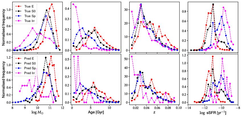
12 M. K. Cavanagh et al.

Figure 11. Similar plot as in Figure 10, albeit with the addition of the fourth morphological class. The top row plots the true morphologies of the complete
dataset, while the bottom plots predicted morphologies for samples in the testing set as classified by the 4-class CNN as either E (red), S0 (black), Sp (blue) or
Irr+Misc (magenta).

 Table 4. Table of classification accuracies for all five hierarchical classifiers.

 Path Best 3-way Accuracy Best 4-way Accuracy

 E-first 82% 63%

 Sp-first 83% 63%

 Reg+3-way N/A 65%

 Huertas-Company et al. 2019). Here we simply process each sam-
 ple in the test set by passing it through a series of binary CNNs (see
 Figure 5 for the classification accuracies of each). We can perform
 the 3-class classification using two different hierarchical classifiers;
 first, classify between E and S0+Sp, then, given the sample is not an
 elliptical, between S0 and Sp. The second route is to first classify
 between E+S0 and Sp, and then, given the sample is not a spiral,
 between E and S0. In the case of the 4-class classification, the first
 binary CNN is simply E+S0+Sp (Regular) vs. Irr+Misc. Figure 12
 illustrates these two different pathways. We will refer to the pathway
Figure 12. Diagram showing the two different paths in our hierarchical that commences with E vs. S0+Sp as E-first, and E+S0 vs. Sp as
classification tree. In the case of 3-way classification, the first step is ignored. Sp-first. We also classify between the four classes first by applying
To classify between E, S0 and Sp, there are two routes depending on whether the Regular vs. Irr+Misc binary classifier, and then applying our
to first look for ellipticals or look for spirals. The subsequent step is then to direct 3-way CNN (thus two overall steps instead of three). We refer
discriminate between the other two categories. to this as our Reg+3-way classifier. Table 4 lists the best overall
 classification accuracies for each of the five hierarchical classifiers.
 Figure 13 shows the confusion matrices for the hierarchical 3-
indirect method was also explored in an attempt to obtain better way classification with both the E-first and Sp-first pathways. Both
classification accuracies for the irregulars. Here, we use multiple have similar overall accuracies, but the Sp-first path best matches
CNNs to construct a binary decision tree, with which to classify the direct 3-way CNN (Figure 6) with a better 65% S0 accuracy and
samples. This approach has been used in many previous works, comparable E and Sp accuracies. The E-first path, while excellent
fundamentally as part of the Galaxy Zoo (Lintott et al. 2008), as at classifying ellipticals, has a much poorer S0 accuracy, with over
well as in other studies in astronomy involving machine learning a third of true S0s misclassified as ellipticals. This is despite the
(Huertas-Company et al. 2010; Domínguez Sánchez et al. 2018; fact that both the E vs. S0+Sp and E+S0 vs. Sp binary classifiers

 MNRAS 000, 1–18 (2021)

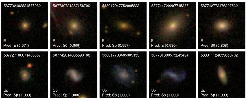
Morphological classification of galaxies 13

Figure 13. Confusion matrices for the 3-way hierarchical classification of ellipticals (E), lenticulars (S0) and spirals (Sp) for the E-first pathway (left) and
Sp-first pathway (right) (see Figure 12 for an overview of these pathways).

Table 5. Table of per-class classification accuracies for the three 4-way ter spread of accuracies across all the categories. The Reg+3-way
hierarchical classifiers (E-first, Sp-first and Reg+3-way). CNN offers a further marginal improvement.
 These results show that indirect, hierarchical classification can
 CNN E S0 Sp Irr offer comparable accuracies to direct 3-way classification, but per-
 forms poorly when compared to direct 4-way classification. Al-
 E-first 91% 33% 63% 90% though the direct CNNs outperform the hierarchical classifiers, the
 Sp-first 76% 45% 64% 90% 3-way Sp-first classifier offers a 5% improvement in S0 classifica-
 tion accuracy.
 Reg+3-way 80% 46% 65% 90%

 4.4 Galaxy Morphology
have similar >90% accuracies. The disparity is reflective of a more Galaxies exhibit an array of fine morphological structure, from
deeper issue: the fact that ellipticals and S0s are inherently much spiral arms, dust lanes and stellar bars, to tidal tails and/or tidal
harder to disentangle, compared to distinguishing between spirals interaction (Conselice 2014). The power of CNNs lie in their abil-
and S0s (compare the 82% and 88% binary classification accuracies ity to extract features in images. As can be seen in the example in
in Figure 5). This may seem counter-intuitive; after all, if Sp are Figure 4, the convolutional layers are able to outline, trace and de-
able to be accurately picked up, then the remaining E+S0 samples tect the presence of spiral arms. The process of visual classification
should have a worse accuracy. The key point is that this is dependent relies on being able to detect and categorise such morphological
on the percentage of true spirals. Spirals are able to be differentiated features (Buta 2013). In general, S0 galaxies are difficult to visually
between E and S0 with 98% and 88% accuracies respectively, so distinguish (Blanton & Moustakas 2009), in part since they exhibit
fewer false positives will progress to the next stage in the hierarchical morphological characteristics that, insofar as solely examining an
tree. However, because E vs. S0 has a lower accuracy, more false image is concerned, are near identical to ellipticals. S0s can also dis-
positive ellipticals (in particular, true S0s falsely classified as E) play prominent dust lanes, rings and large disc components, which
will emerge from the first E vs. S0+Sp stage. Hence the E-first path make them visually similar to spirals, especially in the edge-on case.
results in a greater spread of samples, while the Sp-first path is It is thus expected that the overall CNN classification accuracies are
more accurate at picking up true S0s. For both the Sp-first pathway lower for S0s. Although the networks were trained on single-band
in Figure 13 and the direct 3-way CNN in Figure 6, more true images (g-band), for the purpose of illustrations all examples in the
ellipticals are misclassified as S0s compared to true spirals. figures of this section are the colour image cut-outs taken directly
 Table 5 shows the per-class classification accuracies for each of from SDSS DR4.
our 4-way hierarchical CNNs. Note from Table 4 that the E-first and Figure 14 shows a random selection of galaxies, from each mor-
Sp-first had similar overall accuracies (63%), with a slightly higher phological class, that were correctly identified by the CNN. Most of
65% for the Reg+3-way CNN. Adding an explicit step to classify ir- these samples were classified with a near-certain confidence (>0.99).
regulars has dramatically improved the classification accuracy from Although the ellipticals and S0s in Figure 14 look visually similar,
27% to 90%, but this has come at the severe cost of reduced accu- the CNN is able to distinguish between the two types, possibly by
racies for other classes. This suggests that the more steps there are being able to detect the more prominent bulge and/or evidence of
in the pathway, the harder it is to classify the classes in the later disc-like structure as seen in the S0s. Figure 15 shows a selection
steps. Although the E-first 4-way CNN can classify ellipticals with a of fifteen randomly chosen samples that were misclassified with a
91% accuracy, the S0 accuracy is the lowest out of the three (33%). relatively high confidence, at least >70%. The first three samples
The overall Sp and Irr classification accuracies are similar across (starting from the top-left and moving across to the right) are all
all three classifiers, with the Irr accuracy unchanged. As with the S0s that were misclassified as spirals. All three exhibit fine mor-
3-way hierarchical classifiers, the Sp-first approach provides a bet- phological structure, such as a prolate bulges and stellar bars, and

MNRAS 000, 1–18 (2021)

14 M. K. Cavanagh et al.

Figure 14. Randomly selected galaxy samples from each of the 4 morphological classes that were correctly classified by the CNN. Each image is annotated,
from top to bottom, with its SDSS JID, actual morphological class, and predicted morphological class, with the CNN prediction confidence given in parentheses.

there are hints of faint spiral arms in each. Whether such arms are sified with confidences less than 70%. These examples include sam-
truly well established enough to consider the galaxy a spiral is de- ples that were both correctly and incorrectly classified, and can help
batable, but these examples show that the CNN is able to both detect reveal where most of the confusion is based. In general, compared
their presence and classify accordingly. J100944.44+525738.87, an to Figures 14 and Figures 15, there is far less variety in large-scale
elliptical classified as an S0, demonstrates the difficulty in distin- morphology, and instead distinctions must lie in finer-scale mor-
guishing between these two types by image alone. There are also phologies as well as foreground/background features. The sample
examples of clear confusion; the first two samples in the middle images containing foreground objects in Figure 16 tend to result
row, J023153.52+011234.22 and J082351.91+421319.51, are both in lower confidences, most spectacularly with the first example,
barred galaxies. They have a dataset classification of S0 and Sp re- J075634.20+301032.46. The last two examples in the second row,
spectively, but have been classified by our CNN as opposites (Sp and J004227.71-084550.76 and J144725.16+032627.94, both near vi-
S0, respectively). The CNN has also misclassified all the irregular sually identical, have dataset classifications of S0 and E respectively,
samples in Figure 15 as spirals. Since the network is only trained but both have been classified by the CNN as ellipticals with 49%
on g-band images, the prominent blue colour of the irregulars that and 51% confidence respectively. What is also important to note is
enables the naked eye to easily distinguish that morphological type the uncertainty that surrounds the classification of edge-on galax-
is instead lost to the CNN. One other interesting example is that of ies. In particular, the middle image in the top row of Figure 16
J112459.22+641850.57, a spiral galaxy with extremely faint arms and the first image in the second row (J172421.13+583341.57 and
that arguably looks like a stellar ring, which the CNN has classified J115613.87+034017.46) are both edge on galaxies, and they have
as an S0. both been classified as spiral galaxies. Indeed, since many spiral
 galaxies have prominent discs, from pure population statistics alone
 Figure 16 shows a random selection of samples that were clas-

 MNRAS 000, 1–18 (2021)