Multi-Tier Adaptive Memory Programming and Cluster- and Job-based Relocation for Distributed On-demand Crowdshipping
←
→
Page content transcription
If your browser does not render page correctly, please read the page content below

Multi-Tier Adaptive Memory Programming and Cluster- and Job-
        based Relocation for Distributed On-demand Crowdshipping
                                          Tanvir Ahamed1, Bo Zou.
      Department of Civil, Materials, and Environmental Engineering, University of Illinois at Chicago

Abstract: With rapid e-commerce growth, on-demand urban delivery is having a high time especially
for food, grocery, and retail, often requiring delivery in a very short amount of time after an order is
placed. This imposes significant financial and operational challenges for traditional vehicle-based
delivery methods. Crowdshipping, which employs ordinary people with a low pay rate and limited
time availability, has emerged as an attractive alternative. This paper proposes a multi-tier adaptive
memory programming (M-TAMP) to tackle on-demand assignment of requests to crowdsourcees with
spatially distributed request origins and destination and crowdsourcee starting points. M-TAMP starts
with multiple initial solutions constructed based on different plausible contemplations in assigning
requests to crowdsourcees, and organizes solution search through waves, phases, and steps, imitating
both ocean waves and human memory functioning while seeking the best solution. The assignment is
further enforced by proactively relocating idle crowdsourcees, for which a computationally efficient
cluster- and job-based strategy is devised. Numerical experiments demonstrate the superiority of M-
TAMP over a number of existing methods, and that relocation can greatly improve the efficiency of
crowdsourcee-request assignment.
Keywords: On-demand crowdshipping, Multi-Tier Adaptive Memory Programming, Crowdsourcee-
request assignment, Cluster- and job-based relocation, Multiple knapsack problem

1
    Corresponding author. Email: tanvir.ahamed@hotmail.com
                                                       1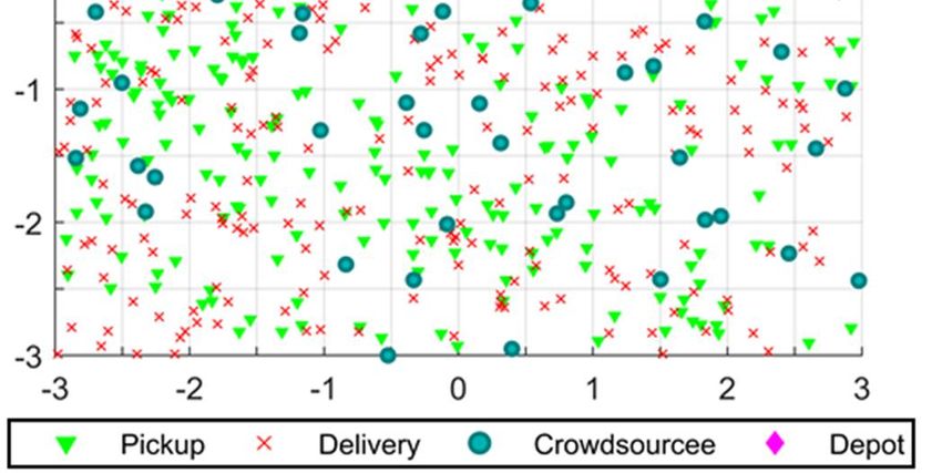
1 Introduction
    E-commerce has experienced unprecedented growth in the recent years. In the US alone, e-
commerce sales achieved $513 billion in 2018, or 9.6% in total retail sales and a 14.3% increase just
from the previous year (US census, 2019). The amount of online sales is projected to continue and
reach $669 billion by 2021 (Statista, 2018) which accounts for 13.7 percent of all retail sales in US
(Statista, 2017). The rapid development of e-commerce along with the fact that the majority of e-
commerce sales occurs in cities and increasingly on-demand suggests considerable increase in delivery
traffic. Relying still largely on vehicle asset-based business models, it means more dispatching of
delivery vehicles, which results in many negative consequences including increased VMTs, traffic
congestion, illegal street parking, greenhouse gas emissions, air pollution, and wear-and-tear of road
infrastructure, which are increasingly at odds with the need and trend of developing livable and
sustainable urban environment.
    The increasing on-demand nature of city logistics, especially among deliveries of food, grocery,
and retail, has imposed considerable pressure on delivery service providers (DSP) to control logistics
cost while meeting the customer demand. These deliveries are often of small size, and from distributed
origins (restaurants, grocery stores, and retail shops rather than the DSP’s warehouse) to distributed
destinations (customers in residence or workplaces). It has become increasingly popular that customers
want to receive the delivery after an order is placed within half to a few hours. Given the vast volume
of such orders, it would be operationally and financially impractical for DSPs to constantly dispatch
self-owned vehicles for pickup and delivery of such services. This is because, first of all, the number
of self-owned vehicles is unlikely to be sufficient to meet the demand. Even if a DSP has enough
vehicles, it would be too expensive to do so.
    As a result of the pressure, innovations are being pushed to meet the growing on-demand, small-
size, and distributed demand with short, guaranteed delivery time. Among the innovations,
crowdshipping has emerged as an attractive, low-cost alternative. In crowdshipping, a DSP solicits
ordinary people, termed crowdsourcees who have available time and may walk, bike, or drive to
perform delivery to earn income. Employing crowdsourcees as ad-hoc couriers often requires a lower
payment rate than full-time employees, thus bringing DSPs significant cost advantage. As
crowdsourcees are either non-motorized or using smaller personal cars, the negative consequences
from DSP-owned truck-/van-based delivery can be largely mitigated. In the business practice,
crowdshipping is rapidly developing with companies like UberEats, Grubhub, DoorDash, Postmates,

                                                  2
Deliv, Piggy Baggy, Amazon Flex, and Dada-Jing Dong Dao Jia reshaping the dinning, e-grocery, and
online retail businesses.
    This paper focuses on developing methodologies for dynamic assignment of requests to
crowdsourcees, and for proactively relocating idle crowdsourcees to mitigate spatial supply-demand
imbalance in the crowdshipping system. As the delivery environment considered in the paper is on-
demand, assignment and relocation decisions need to be made in real time while ensuring the quality
of the decisions. For the assignment problem, while it bears some relevance with the dynamic pickup
and delivery problem with time windows (PDPTW) in the vehicle routing problem (VRP) literature,
the problem does differ in that crowdsourcees have limited and heterogenous amount of available time,
and the time between the generation of a request and the latest delivery of the request is very short. A
novel population- and memory-based neighborhood search heuristic is developed which yields better
results than existing methods for solving PDPTWs. For the relocation problem, given that a real-world
system can involve a non-trivial number of idle crowdsourcees, a cluster- and job-based strategy is
conceived for relocation decisions in a computationally efficient manner. The performance of joint and
periodic assignment and relocation is evaluated in extensive, large-size numerical experiments, with
the results compared with those obtained from using the state-of-the-art methods.
    Three major contributions are made in the paper. First, a novel multi-start, multi-tier adaptive
memory programming (M-TAMP) algorithm is proposed for assigning requests to crowdsourcees in
an on-demand environment. The multiple tiers include decomposing the solution search through
waves, phases, and steps. By doing so, the neighborhood search for better solutions is made more
systematic and effective given the huge number of routing permutations to explore. Strategic
oscillation among solutions is embedded, which allows solutions in the memory to be reexamined,
solutions that repeatedly appear in the memory to be tabued to avoid cyclic search, and currently not-
so-good but promising solutions to be kept in memory for further improvement. We also investigate
the construction of initial solutions for the algorithm, which is shown critical to the search for best
solutions. All these contribute to the computational superiority of M-TAMP over existing methods.
Second, the possibility to improve system responsiveness to new shipping requests and reduce total
shipping cost is investigated. Specifically, a clustering-based strategy is proposed that makes relocation
decisions in a computationally effective and efficient manner. Third, through comprehensive numerical
experiments, a number of managerial insights are offered about crowdshipping system operations to
meet on-demand urban deliveries.

                                                    3
The remainder of the paper is structured as follows. Section 2 reviews relevant literature. A formal
description of the problem for on-demand request-crowdsourcee assignment and idle crowdsourcee
relocation is presented in Section 3. In Section 4, we provide an overall picture of the M-TAMP
algorithm for the assignment problem. This is followed by detailed description of the elements in M-
TAMP in Section 5. Section 6 presents the cluster- and job-based relocation strategy with its
mathematical formulation. Extensive numerical experiments are conducted in Section 7. The findings
of the paper are summarized and directions for future research are suggested in Section 8.

2 Literature review
    Our review of relevant literature is organized in three subsections. First, we review existing
research on planning and operation of crowdshipping systems. Then, methods for solving dynamic
PDPTW, a problem closely resembling our assignment problem, are reviewed. The last subsection
focuses on research on transportation resource relocation, which is relevant to relocating idle
crowdsourcees.

2.1 Crowdshipping system design and operation
    As a result of the rapid development in industry practice, crowdshipping has garnered much
research attention in recent years. Relevant literature considers three aspects: supply, demand, and
operation and management (Le et al., 2019). As our paper concerns the third aspect, the review in this
subsection mainly focuses on different operational schemes and strategies that have been proposed.
    One branch of crowdshipping research works consider crowdsourcees to perform the last leg of
the urban delivery, while propose traditional vehicles to coordinate with the crowdsourcee routes. In
the similar direction, a number of operational concepts have appeared in the literature. Kafle et al.
(2017) proposes a two-echelon crowdshipping-enabled system which allows crowdsourcees to perform
the first/last leg of pickup/delivery while relaying parcels with trucks at intermediate locations. A
mixed integer program (MIP) along with tailored heuristics is proposed to minimize system overall
cost. Wang et al. (2016) formulate a pop station-based crowdshipping problem in which a DSP only
sends parcels to a limited number of pop stations in an urban area, while crowdsourcees take care of
delivery from the pop stations to customers. Focusing on the crowdsourcee part, a minimum cost
network flow model is formulated to minimize crowdsourcing expense while performing the last-leg
deliveries. Macrina et al. (2020) consider that crowdsourcees may pick up parcels from a central depot
or an intermediate depot to which parcels are delivered by classic vehicles. Customers can be served
either by a classic vehicle or a crowdsourcee. Each crowdsourcee serves at most one customer. To
                                                 4
solve this problem, an MIP and a metaheuristic are developed. The use of intermediate transfer
locations is further considered by Sampaio et al. (2018) who propose a heuristic for solving multi-
depot pickup and delivery problems with time windows and transfers, and by Dötterl et al. (2020) who
use an agent-based approach to allow for parcel transfer between crowdsourcees.
    Another branch of crowdshipping research considers not only dedicated crowdsourcees but also
people “on-the-way” (introduced as occasional drivers), who are willing to make a single delivery for
a small amount of compensation using their own vehicles. The static version of this problem is
formulated as a vehicle routing problem with occasional drivers, solved by a multi-start heuristic
(Archetti et al., 2016). The dynamic version is considered in Dayarian and Savelsbergh (2017) solved
by two rolling horizon dispatching approaches: a myopic one that considers only the state of the system,
and one that also incorporates probabilistic information about future online order and in-store customer
arrivals. A rolling horizon framework with an exact solution approach is proposed by Arslan et al.
(2019) which look into dynamic pickups and deliveries using “on-the-way” crowdsourcees. In-store
shoppers are also considered as possible crowdsourcees to perform delivery (Gdowska et al., 2018).
    Recently, an analytic model is developed by Yildiz and Savelsbergh (2019) to investigate the
service and capacity planning problem in a crowdshipping environment, which considers the use of
both crowdsourced and company-provided capacity to ensure service quality. The study seeks to
answer many fundamental questions such as the relationship between service area and profit, and
between delivery offer acceptance probability and profit, and the benefits of integrating service of
multiple restaurants. Recognizing that using friends/acquaintances of the shipping request recipients
makes delivery more reliable, Devari et al. (2017) conduct a scenario-based analysis to explore the
benefits of retail store pickups that rely on friends/acquaintances on their routine trips to
stores/work/home. Similarly, Akeb et al. (2018) examine another type of crowd logistics in which
neighbors of a customer collect and deliver the parcels when the customer is away from home, thereby
reducing failed deliveries.
    Despite the proliferation of research in the crowdshipping field, an efficient solution technique for
dynamic PDPTW, while proactively relocating idle crowdsourcees simultaneously, has not been
considered in the literature as a way to improve the crowdshipping system operations. In addition to
this major gap, there seems to be little attention paid to the limited time availability that dedicated
crowdsourcees are likely to have while performing crowdshipping. This paper intends to address these
gaps.

                                                   5
2.2 Methods for solving dynamic PDP
    As mentioned in Section 1, the crowdshipping problem considered in this paper can be viewed as
an adapted version of dynamic PDPTW, for which the reader may refer to Berbeglia et al. (2010) and
Pillac et al. (2013) for reviews. Given the NP-hard nature of PDPTW, it is not surprising that most
existing solution methods for dynamic PDPTW are heuristics.
    A most widely used heuristic for dynamic PDPTW is tabu search. Two notable works in this field
are Mitrović-Minić et al. (2004) and Gendreau et al. (2006). The former considers jointly a short-term
objective of minimizing routing length and a long-term objective of maximizing request slack time
while inserting future requests into existing routes. The latter employs a neighborhood search structure
based on ejection chain. However, neither of the two studies account for future requests. Ferrucci et al.
(2013) develop a tabu search algorithm to guide vehicles to request-likely areas before arrival of
requests for urgent goods delivery. This work is later extended by Ferrucci and Bock (2014) to include
dynamic events (e.g., new request arrival, traffic congestion, vehicle disturbance).
    Other than tabu search, Ghiani et al. (2009) employ an anticipatory insertion procedure followed
by an anticipatory local search to solve uncapacitated dynamic PDPTW for same-day courier service.
Similar to the idea of Bent and Van Hentenryck (2004) to evaluate potential solutions using an
objective function that considers future requests through sampling. The study exploits an integrated
approach in order to address multiple issues involved in real-time fleet management including
assigning requests to vehicles, routing and scheduling vehicles, and relocating idle vehicles. The
authors find that the proposed procedure for routing construction outperforms their reactive
counterparts that do not use sampling. Besides heuristics, an optimization-based algorithm is proposed
by Savelsberg and Sol (1998) to solve real-world dynamic PDPTW.

2.3 Resource relocation
    To our knowledge, no research exists on crowdsourcee relocation. If we consider idle
crowdsourcees as resources, crowdsourcee relocation resembles the problem of relocating empty
vehicles which has been investigated in a few different contexts. An example is autonomous mobility
systems, in which relocating idle autonomous vehicles can better match vehicle supply with rider
demand (Fagnant and Kockelman, 2014; Zhang and Pavone, 2016). The need for vehicle relocation
also arises in one-way carsharing. Boyaci et al. (2017) and Nourinejad et al. (2015) show the potential
benefit of relocating empty electric vehicles to better accommodate carsharing demand. Sayarshad et
al. (2017) propose a dynamic facility location model for general on-demand service systems like taxis,

                                                   6
dynamic ridesharing services, and vehicle sharing. An online policy is proposed by the authors to
relocate idle vehicles in a demand responsive manner with look-ahead considerations.
    Relocating vehicles has been studied, at least implicitly, for freight movement as well. In the
PDPTW literature, Van Hemert and La Poutré (2004) introduce the concept of “fruitful regions” to
explore the possibility of moving vehicles to fruitful regions to improve system performance.
Motivated by overnight mail delivery services, a traveling salesman problem is investigated by Larsen
et al. (2004) with three proposed policies for vehicle repositioning based on a-priori information.
Waiting and relocation strategies are developed in Bent and Van Hentenryck (2007) for online
stochastic multiple vehicle routing with time windows in which requests arrive dynamically and the
goal is to maximize the number of serviced customers.

3 Problem description
    As mentioned in Section 1, this paper investigates a specific type of on-demand crowdshipping
that the origins and destinations of shipping requests and the starting points of crowdsourcees are all
spatially distributed. A DSP constantly receives requests and uses crowdsourcees to pick up and deliver
the requests within a short, guaranteed period of time (e.g., two hours). Crowdsourcees also
dynamically enter the crowdshipping system. Crowdsourcees have limited available time and will exit
the system when the available time is used up. Each crowdsourcee can carry multiple requests as long
as their carrying capacity allows. Crowdsourcee routes can be dynamically adjusted as new incoming
requests are added at the end or inserted in the middle of the routes. With proper payment as incentives,
idle crowdsourcees can move from their current locations to new locations suggested by the DSP. The
relocation is to benefit the DSP by reducing its total shipping cost (TSC).
    In this paper, we consider that the DSP performs periodical crowdsourcee-request assignment,
each time with the latest information about unassigned shipping requests and crowdsourcees, who can
be either idle or en route, carrying previously assigned requests. As such, a request can be inserted at
the end or middle of an existing crowdsourcee route. Alternatively, a request may be given to an idle
crowdsourcee. After a request is generated, it will be considered at the next immediate assignment.
However, it is possible that some requests cannot be assigned to any existing crowdsourcees as
feasibility and/or pickup distance constraints are violated (see subsection 5.1). In this case, a request
may be picked up and delivered by a backup vehicle if urgent, or left for the next assignment.
    Each time an assignment is made, decisions on relocating idle crowdsourcees are made right after.
Compared to instant assignment whenever a new request or a new crowdsourcee enters the system,

                                                   7
periodic treatment can take advantage of accumulated information during the inter-assignment period
to make assignment more cost-effective. The period certainly should not be too long given that each
request has a delivery time guarantee. The extent to which the inter-assignment period length on system
performance will be investigated in future computational experiments.

4 M-TAMP algorithm for request-crowdsourcee assignment: Overall
    picture
4.1 Fundamental idea
    The proposed M-TAMP algorithm is a multi-start, population- and memory-based neighborhood
search heuristic. The algorithm starts from multiple initial solutions constructed based on different
plausible contemplations for assigning requests to crowdsourcees. Through neighborhood search, a
growing number of alternative solutions are generated and evaluated in an iterative manner, with a
portion of them selected to enter an adaptive memory (          ) in which solutions are constantly updated
and direct further solution search. The selection of solutions to enter/update AM is probabilistic, thus
allowing some currently not-so-good but maybe promising solutions to be selected, which may get
substantially improved in subsequent search.       plays the role as a container of good and not-so-good
but maybe promising solutions which, like human memory, evolves in the course of the search.
Solutions that show repeated appearance will be permanently kept (tabued) in           .
    The novelties of the M-TAMP heuristic lie in three parts: 1) structuring the solution search by
constructing sequential and interconnected waves. Each wave is associated with removing requests
from one route and inserting the removed requests to other routes; 2) structuring each wave by
alternately performing vertical and horizontal phases. A vertical phase pertains to adding solutions to
   , whereas a horizontal phase reexamines solutions in           ; 3) structuring each horizontal phase by
conducting removal-replacement of         solutions in multiple steps. Below we provide more detailed
(though still conceptual) elaboration of the three novelties.
    For the first novelty, given that a solution entails a number of routes, instead of improving all
routes simultaneously, the M-TAMP heuristic focuses on one route at a time, by moving a request from
the route of focus to another route. As there exist many possibilities for a move (considering many
requests in the route of focus and many positions in other routes to insert the moved request), only a
portion of the possibilities will be selected for consideration. Such a decomposition and solution
improvement by focusing on one route at a time prevents dealing with a huge number of neighborhood

                                                    8
search all at once, which would be computationally expensive and cumbersome, and lead to the
algorithm losing focus in search. This is particularly important as memory is involved in the search.
Too many solutions all appearing at the same time will just render the probability of solution
reoccurrence very unlikely. In addition, the sequential nature of the decomposition, i.e., solutions
resulting from focusing on one route will be used for generating new solutions when focus is shifted
to the next route, allows the search efforts made earlier to be used in subsequent routing improvement.
The idea of route improvement by focusing on one route at a time is akin to ocean waves lapping at
the shore one after another, thus. This explains the use of the term “waves”.
    For the second novelty, a multitude of permutations exists in each wave because many possibilities
exist for picking up a request to remove from the route of focus and inserting the removed request in
another route. Exploring all possibilities at once will be computationally expensive. In addition, doing
so would generate a vast number of solutions which can result in exceeding randomness in selecting
solutions to enter    . Instead, M-TAMP organizes the search by performing routing improvement in
consecutive, alternating vertical and horizontal phases. A vertical phase adds solutions to          (thus the
length of     is vertically expanding), whereas a horizontal phase reexamines the solutions in                by
removing each solution and replacing the solution with another solution probabilistically selected from
   . In a vertical phase, before selecting a solution to enter                , M-TAMP also explores an
improvement possibility by removing/inserting one more request for the solutions selected. Iteratively
performing solution addition in vertical phases and removal/replacement in horizontal phases follows
the idea of a strategic oscillation (Glover and Laguna, 1997a and 1997b), which allows for reexamining
the solutions in     . By doing so,       gets updated and evolves based on the latest neighborhood
search towards better solutions.
    For the third novelty, in a horizontal phase the removal-replacement operation involves removing
each solution from     , returning the solution to        , and probabilistically selecting a solution from
and add the solution to the end of     (i.e., replacement). The purpose is to reexamine the solutions in
   : if a solution is inferior (high TSC), then the chance of getting the solution back by probabilistic
selection is low. Thus, such solutions are removed from              and replaced by better solutions. For a
good solution (low TSC), getting it back to          is still likely through probabilistic selection. As new
solutions are constantly added to      , the removal-replacement operations updates                 by giving
chances for good solutions that appear later in           to replace earlier solutions in      . To avoid the
cycling of removing solutions that have repeatedly entered               , we tabu solutions with sufficient
reoccurring frequency in       . In performing the removal-replacement, each horizontal phase is
                                                      9
decomposed into multiple steps, each step performing removal-replacement on only a portion of the
solutions in    . Doing so helps currently not-so-good but maybe promising solutions to get a chance
to be selected from     to enter      . This is because, by removing a fraction of     solutions at a time
and adding them to      , the influence of new       solutions on selecting an existing solution in     is
limited. This is desirable as it preserves the chance to enter solutions in      that are currently not so
good but could get improved in subsequent waves. Otherwise, removing                 solutions all at once
would result in decreased chance for existing solutions in       to be selected, especially when the
solutions have low TSC.

4.2 Difference of M-TAMP from existing metaheuristics
    It is worth highlighting the difference between the M-TAMP algorithm and some existing
metaheuristics: genetic algorithm (GA), simulated annealing (SA), and tabu search (TS), which have
been widely used in combinatorial optimization including VRP/PDPTW. GA and SA do not involve a
memory. For GA, it starts with an initial population of solutions and then iteratively performs genetic
operators including crossover and mutations to produce offspring solutions. For efficient search for a
given problem, tuning parameters is critical but non-trivial (Smit and Eiben, 2009). SA relies on a
single solution in the search. Mimicking the cooling process of materials, SA requires the cooling rate
to be very slow when a number of local minima are scattered in the solution space. This is in contrast
with the computational requirement for dynamically solving PDPTW in the on-demand delivery
context.
    TS exploits memory structures in combination with strategic restrictions and aspiration levels as
a means for exploring the search space (Glover et al., 1995). There are different types (e.g., classical
TS, reactive TS, threshold-based TS, etc.) in the literature. The literature suggests that the solution
quality depends on the value of the tabu tenure, i.e., duration that an attribute tabued to avoid cyclic
exploration (Glover, 1995). If the tabu tenure value is set too high, then the search will be confined to
a specific region of the search space. If the value is set too low, then the chance of cycling in solution
exploration will increase, compromising computational efficiency. Research on this topic is abundant
but still needs further development to present a robust and deterministic tabu scheme. In addition, while
the concept of tabu-list in TS bears a resemblance to AM, the use and construction mechanism of AM
(remove-replace) is very different.

                                                    10
4.3 Overall flow of M-TAMP
Following the idea discussed above, this subsection provides further details about the M-TAMP
algorithm, graphically shown in Fig. 1 and procedurally exhibited in Algorithm 1 below. Table 1
provides the notations used in this subsection and Section 5.
Table 1. Notations used in the M-TAMP algorithm and their definitions
Lists and Sets
Candidate list of routing solutions
Temporary candidate list, which is a set of routing solutions
List of solutions in the adaptive memory
Set of solutions that have entered more than a certain number of times
Variables
Initial solution
Shipping cost of solution
Guaranteed delivery time
, Travel time on a route of a solution
, Amount of lateness for delivery with respect to the delivery time guarantee for all
the assigned requests in the routes of a solution
, Amount of time violation with respect to the available time window over all
crowdsourcees for a solution
, Total number of requests that exceed the carrying limits over all crowdsourcees for
a solution
Pr( ) Probability of selecting a candidate solution
Selected candidate solution from to apply forward move
Selected solution in the vicinity of the selected solution ( )
Generated forward move by application of intra-route move on
Best solution after improvement of initial solution using M-TAMP
Best solution cost after improvement of initial solution using M-TAMP
Parameters
Parameter that emphasizes or de-emphasizes the cost reduction potential of a
solution
Number of solutions in during phase
ℎ Number of horizontal steps required during phase
, Number of remove/replace move required from/to during a horizontal step of
a phase
Parameter that facilitates the calculation of number of phase reqd. ( ∗ )
Separation between successive values
11Generate initial solutions
Iterate over waves
Generate and update
candidate list ( )
Set parameter values
Vertical phase
Iterate over phases
Select solutions from
Perform forward moves
Add solutions to adaptive memory ( )
Horizontal phase
Remove
Remove a portion of solutions
from the top of
Return the solutions to if
they do not exist in
Iterate over steps
Replace
Probabilistically select the same
number of solutions from CL as
those returned from
Add solutions to the end of
Update best solution
Concluding horizontal phase
Fig. 1. Flow of the M-TAMP algorithm.
12The structure of the M-TAMP, as discussed above, is formalized as Algorithm 1. The inputs of
the algorithm are: the total number of initial solutions ( ); the total number of existing crowdsourcee
routes ( ); the number of solutions to be added to AM during intervention ( ); the number of
∗
horizontal steps during phase (ℎ ), ∀ = 1, … , ; and the number of solutions to remove/replace
( , ) during horizontal step of phase . The output of the algorithm is the best routing solution of
crowdsourcees who are assigned with shipping requests ( ).
Algorithm 1. M-TAMP algorithm
Input: , , ,ℎ , ,
Output:
1. begin procedure
2. ←∞ ⊳ Initialize DSP total shipping cost
3. for = 1, … , ⊳ Consider multiple initial solutions
4. ← Generate an initial solution ⊳ See subsection 4.3.1
5. ←∅ ⊳ Initialize adaptive memory
6. for = 1, … , ⊳ Wave counter
7. ← Generate a candidate list of solutions ⊳ See subsection 4.3.2
8. Set values for , , , ℎ ⊳ See Appendix A
9. ← ∪ ⊳ Adding solutions in to
10. for = 1, … , ∗ ⊳ Phase counter
11. if | |< then
12. ℎ , ,
13. else
14. ℎ , ,ℎ , , ,
15. end if
16. ← min ⊳ Solution with lowest TSC in
∈
17. if > then
18. ←
19. end if
20. end for
21. Perform concluding horizontal phase
22. end for
23. end for
24. return
25. end procedure
135 Elements of the M-TAMP algorithm
5.1 Generating initial solutions
Each time an assignment is performed, M-TAMP involves generating an initial solution first, i.e.,
perform an initial assignment of each new request to an available crowdsourcee, and then improving
the solution. Except for the beginning of the day, the available crowdsourcees for an assignment consist
of two types: 1) those who are idle; and 2) those who have assigned requests which are not yet
completed, but still have some available time to be assigned more requests. In generating an initial
solution, new requests are first added, one at a time, to the end of a crowdsourcee route. Intra-route
move is then applied to the added request to obtain the routing sequence with the lowest cost. In this
paper, we propose three methods to generate initial solutions based on urgency of a request;
crowdsourcee availability of a request; and time availability of a crowdsourcee respectively. Therefore,
M-TAMP will start from three initial solutions at each assignment period. The best subsequent solution
resulting from the three initial solutions will be chosen for the actual assignment.
A few constraints need to be respected in generating initial solutions. First are feasibility
constraints: 1) all requests must be delivered within the guaranteed delivery time; 2) the time to
complete a route should not exceed the available time of the crowdsourcee; and 3) the weight carried
should not exceed the carrying capacity of the crowdsourcee. In addition, we assume that a
crowdsourcee picks up requests only within a distance threshold. Specifically, if a crowdsourcee is
idle, the pickup distance of a request is the distance between the pickup location and the current
location of the crowdsourcee. If the assigned crowdsourcee is already en route, the pickup distance
would be the distance between the end of the pickup location and the existing route.
The first method to generate an initial solution is based on slack time of each request , which is
calculated as the difference between the latest possible pickup time + − , and the current
time , where is the time when request is generated; is the guaranteed delivery time (e.g., 2
hours) of the request; and , is the crowdsourcee travel time from the pickup to the delivery location
on direct route. This calculation, inspired by Mitrović-Minić and Laporte (2004), means that the
smaller the slack time, the more urgent a request needs to be delivered. Thus the requests are assigned
in order of their urgency to crowdsourcees while satisfying the constraints mentioned above. For a
given request, the closest crowdsourcee is considered first. If not possible, then the second closest
crowdsourcee, and so on. Once a request is assigned, the time availability of the assigned crowdsourcee
will be updated. If a request cannot be assigned to any crowdsourcee, it will be labeled and put aside.
14After all requests are checked, unassigned requests that cannot wait any further will be assigned
to back-up vehicles which depart from a central depot. A request cannot wait any further if it would be
too late to pick up and deliver the request using a backup vehicle at the next assignment period. To
ensure speediness, in this paper we assume that each unassigned request will be picked up and delivered
by a dedicated back-up vehicle. Unassigned requests that can wait will be left for assignment in the
next assignment period.
The second method to generate an initial solution is based on crowdsourcee availability. The idea
is to give requests with more limited crowdsourcee availability high priority. Requests are ordered by
the number of available crowdsourcees who are within the pickup distance threshold. We look for
crowdsourcees to assign for those requests with just one available crowdsourcee, and then requests
with two available crowdsourcees, and so on. If two requests have the same number of available
crowdsourcees, they are further prioritized based on when they are generated. Similar to the first
method, for each request the closest available crowdsourcee is examined first. If not possible to be
assigned, then the second closest, etc. Requests that cannot be assigned to any available crowdsourcee
will be labeled and put aside. After all the requests are checked, the labeled requests will be similarly
treated as in the first initial solution.
The third method considers assigning crowdsourcees instead of requests. Crowdsourcees are
assigned in a descending order of available time. The argument for a descending order is that
crowdsourcees with greater time availability are more “valuable” considering their possibilities to
accommodate future requests. For a given crowdsourcee, we check if the nearest request can be added
to meet the feasibility and pickup distance constraints. If added, we update the crowdsourcee’s
available time and proceed to the crowdsourcee with the highest time availability (which could be the
same crowdsourcee if his/her available time is sufficiently large). If adding the request is not possible,
we examine the next closest request, and so on. For those requests that end up not assigned, we check
again if a request needs to be assigned to a backup vehicle right away or can wait till the next
assignment period.
5.2 Generating a candidate list of solutions
As mentioned before, once an initial solution is generated for an assignment period, we proceed
sequentially with the first wave, the second wave, and so on. The way each wave works is similar and
built on the best routing solution of the previous wave. Without loss of generality, the discussion below
focuses on the first wave. The first step of a wave is to generate a candidate list of solutions using the
initial solution.
15Specifically, we remove each request from the route of the wave one at a time. The removed
request is added to the end of another route, with intra-route move subsequently performed to generate
solutions in the . To illustrate, suppose we have three routes. A wave is associated with route 1
which has three requests. 3 × 2 = 6 solutions are first generated (i.e., removing each of the three
requests from route 1 and adding the request to the end of the other two routes). For each of the six
solutions, the added request is further moved to an earlier position in the route. This procedure yields
a set of alternative solutions. To quantify the attractiveness of a solution , Eq. (1) is used to look at
its TSC:
=∑ , + , + , + , (1)
In Eq. (1), TSC is expressed in the amount of time involved. ∑ , denotes the total travel
time over all crowdsourcee routes = 1, … , . , represents the amount of lateness of deliveries
with respect to the guaranteed delivery time of the requests. , indicates the amount of time
violation with respect to the available time window of crowdsourcees. , denotes the total excess
weight carried by crowdsourcees. , , and are parameters describing the extent of penalty for the
three different types of feasibility violation. also serves to convert the excess weight to time.
Note that the calculation of permits some feasibility constraint to be violated for a solution.
We keep some infeasible solutions as they could get improved in M-TAMP. However, if a solution is
too inferior, i.e., the cost difference between the solution and the initial solution is too large, it will be
discarded. Three pruning techniques are further applied to delete infeasible solutions. First, if the
request is too far away from other nodes on the route where the request is moved preventing on-time
delivery of the request even by putting the request as the top priority for pickup and delivery, the
solution will be deleted. Second, a solution will be pruned if the travel time from any unserved node
on the route where the request is moved to the pickup node of the request exceeds the pickup
distance threshold, and it is not possible to move another request from a different route to meet the
pickup distance threshold while satisfying the feasibility constraints. Third, a solution will be
pruned if the crowdsourcee of the route where the request is moved ends his/her available time
earlier than the appearance of a request. The remaining solutions after pruning form the candidate
list.
165.3 Vertical phase
A vertical phase deals with adding solutions to using solutions in as inputs. The pseudo
code is shown in Algorithm 2. The inputs of a vertical phase are: current , the number of solutions
required to enter in the phase ( ), and . The output is an updated . We iteratively select
solutions one from at a time (line 3) and perform a forward move (line 5) on each selected solution.
The selection of solutions from is probabilistic based on cost difference from the initial solution
using a Logit-type formula (Eq. (2)). The greater the cost reduction a solution is compared to , the
more likely is selected. Compared to deterministic selection strictly by TSC, probabilistic selection
permits diversification: not-so-good solutions in get a chance to be selected, explored by a forward
move, and enter .
( )= (2)
∑ ∈
where is a parameter which can emphasize ( > 1) or de-emphasize ( < 1) the cost difference.
In Algorithm 2, a forward move (line 4) is performed to improve the selected solution by further
exploring its neighborhood. Specifically, after a solution is selected, we remove one more request
from the route associated with the current wave and add the removed request to the end of any other
routes, thus generating a set of new solutions.
Algorithm 2. ℎ (for phase )
Input: , ,
Output: Updated
1. begin procedure
2. while | |<
3. ← Select a solution from using Eq. (2)
4. ← Forward move on
5. Update
6. Update
7. end while
8. return
9. end procedure
For example, suppose we have three routes and route 1 is associated with the current move. After
generating the initial , only two requests remain in route 1. Then four (2 × 2) new solutions will be
17generated. A solution will be selected, termed , from the four solutions using Eq. (2). Intra-route
moves are then performed on the route to which the request is added. The resulting solution with the
least TSC (termed ) will be picked. If < , then enters and remains in .
Otherwise, enters and also remains in . enters . Solutions in are ordered by their
times of entry. For a forward move during a wave, if the candidate list is empty or if the associated
route is empty we do not perform the forward move.
5.4 Horizontal phase
Once the prespecified number of solutions enters in a vertical phase, a subsequent horizontal
phase is triggered which scrutinizes solutions in in the order of their time of entry. Specifically,
we check if a solution can be removed from , returned to , and replaced with a solution selected
from . This procedure is termed as “removal-replacement”. As shown in Algorithm 3, the inputs for
a horizontal phase are: adaptive memory and candidate list, the number of horizontal steps to perform
(ℎ ), the number of solutions to remove/replace ( , ) in horizontal step of phase ; and the set of
solutions that have entered for a sufficient number of times ( ). The output of the algorithm is
an updated after scrutinizing existing solutions. A horizontal phase is divided into multiple steps
ℎ (line 2) each performing removal-replacement on a subset of solutions in . For a given step, if
the solution at the top of has not appeared in enough times (line 6), we return the solution to
and remove it from (lines 7-8). Note that if a solution is already in , then “return” does not
lead to any change to .
If a solution has appeared in enough times, we believe that the solution is attractive enough
and move it to the end of (lines 10-12). After all solutions are considered in a step, we add the
same number of solutions to the end of as the number of solutions removed from in the step
(lines 16-22). The added solutions are probabilistically selected from and should not be those
already in (lines 17-18). Each time a new solution is added to , is updated. After all
horizontal steps are performed in a horizontal phase, is returned for the next vertical phase (line
24).
The removal-replacement procedure updates toward better solutions through three aspects.
The first aspect is reducing the probability of getting an inferior solution back to . The “return”
operation adds new good solutions generated from forward moves in the previous vertical phase to .
Thus more terms will appear in the denominator of Eq. (2). Consequently, the probability of selecting
an inferior solution becomes even smaller. This aspect indeed mimics human brains in that as a person
18spends time searching for good solutions, he/she will naturally encounter many solutions. When the
number of solutions gets larger, it will become more difficult for those not-so-good solutions to come
back to the person’s memory again.
Algorithm 3. ℎ (for phase )
Input: , ,ℎ , , ,
Output: Updated
1. begin procedure
2. for = 1, … , ℎ ⊳ is horizontal step indicator during intervention
3. =0 ⊳ records the number of solutions removed from in a step
4. =1 ⊳ is solution indicator during horizontal step
5. while ≤ , ⊳ , is the number solutions at the top of list that are to
be checked during horizontal step
6. if [1] ∉ ⊳ Check if the solution on top of the list has
entered enough times
7. ← ∪ [1] ⊳ If not, add the solution back to
8. ← \ [1] ⊳ Remove the solution from the top of list
9. = +1
10. else ⊳ If the solution on top of the list has entered
enough times
11. [| | + 1] = [1] ⊳ Add the solution to the end of the list
12. ← \ [1] ⊳ Also remove the solution from the top of list
13. end if
14. = +1
15. end while
16. for = 1, … ,
17. if ∃ ∈ such that ∉ ⊳ Check if there exists one solution in that
can be added back to
18. ← Select a solution from using Eq. (2)
19. [| | + 1] = ⊳ Add selected solution to the end of list
20. Update
21. end if
22. end for
23. end for
24. return
25. end procedure
For the second aspect, the use of tabus persistently attractive solutions which are characterized
by having appeared in enough times, sparing search effort for diversification, i.e., investigating
other less explored solutions. This aspect also imitates human memory: in searching for good solutions,
solutions that have come across one’s head a sufficient number of times will “register” in the person’s
19memory and thus cannot be erased easily. The repeatedly appearing solutions are also likely to be
solutions of relatively good quality.
The third aspect relates to dividing a horizontal phase into steps, to increase the chance for not-
so-good but maybe promising solutions to be selected from into . As each step only contains a
subset of solutions in , some very good solutions in , for example those generated from forward
moves in the preceding vertical phase, will be deferred to later steps. The “return” operation in the
current step then will give greater probability to those not-so-good but promising solutions in to be
selected into . This step-wide operation ultimately helps preserve not-so-good but promising
solutions in at the end of a wave, allowing such solutions to be explored further in future waves.
Like the previous two aspects, this aspect is similar to human memory functioning: sometimes a person
wants to keep both the best solutions found so far and some currently less good solutions as alternatives
in hopes for significant improvement in the future.
5.5 Concluding horizontal phase
The purpose of the concluding horizontal phase is to re-examine solutions after the last horizontal
phase. The difference between the concluding horizontal phase and a horizontal phase is that in a
horizontal phase we remove and replace same number of solutions, whereas in the concluding
horizontal phase solutions in are replaced until a boundary solution is found (no more selection
from or forward move possible for a solution selected from ).
6 Relocating idle crowdsourcees
The efficiency of the above request-crowdsourcee assignment can be improved with balanced
spatial distribution between available crowdsourcees and unassigned requests. However, such balance
is unlikely to persist in a crowdshipping system considered in the paper. Recall that the request pickup
locations are restaurants, grocery stores, and retail shops which are likely to concentrate in downtown
or district centers of a city. In contrast, delivery locations would be residential locations spreading
across a city. As a consequence, overtime fewer crowdsourcees will be around the pickup locations of
requests. It could also occur that some request pickups are from unpopular locations far away from
available crowdsourcees. The imbalance prompts the DSP to use more backup vehicles for guaranteed
delivery, resulting in higher TSC.
Proactively relocating idle crowdsourcees in view of unfulfilled and anticipated future demand
can mitigate the spatial imbalance. Doing so can also improve crowdsourcee responsiveness. For
example, a crowdsourcee relocated in advance to locations close to anticipated requests reduces the
20travel time for pickup after assignment. However, no efforts have been made in the crowdshipping
literature to investigate the issue of crowdsourcee relocation. This section considers relocating idle
crowdsourcees between zones which are sub-units of the overall service area. We assume that monetary
incentives will be provided for idle crowdsourcees to relocate. Conceptually, an ideal relocation should
pursue two objectives that are at odds: 1) minimizing spatial imbalance between request demand and
crowdsourcee supply; and 2) minimizing relocation cost. The relocation decision also requires careful
consideration of the heterogeneity of the available time among idle crowdsourcees, and how to best
use the available time by matching one idle crowdsourcee with multiple unassigned requests while
being relocated.
6.1 Upper bound for the number of relocatable crowdsourcees
This subsection focuses on finding an upper bound of the number of relocating crowdsourcees.
The upper bound is sought assuming that each relocating crowdsourcee would be assigned one request
in the zone where he/she is relocated. The upper bound is useful by itself as well as for determining a
more cost-effective relocation strategy (subsection 6.2) in which a relocated crowdsourcee can be
assigned multiple requests.
We consider that the DSP decides what idle crowdsourcees to relocate right after each assignment,
to improve the spatial crowdsourcee-request balance for the next assignment. The relocation also
anticipates new arrivals of requests and crowdsourcees. Specifically, after an assignment time , we
estimate for each zone the numbers of idle crowdsourcees ( , ∆ ) and unassigned requests ( , ∆ )
right before the next assignment at + ∆ . , ∆ is the sum of three terms:
, ∆ = , + , ∆ + , ∆ (3)
where , is the number of idle crowdsourcees in zone right after assignment at . , ∆ is the
number of crowdsourcees who are en route at but will finish the assigned delivery trips or relocation
trips (which started before ) and become available in zone at + ∆ . , ∆ is the expected number
of new crowdsourcees arriving in zone between and + ∆ .
, ∆ is the sum of two parts:
, ∆ = , + , ∆ (4)
21where , is the number of unassigned requests in zone right after assignment at . , ∆ is the
number of new requests arriving in zone between and + ∆ .
Without relocation, the net excess of crowdsourcees ( , ∆ ) and requests ( , ∆ ) in zone right
before the next assignment at + ∆ can be expressed as Eq. (5)-(6). Obviously, only one of , ∆
and , ∆ can be positive (both could be zero).
exc
, +∆ = max , +∆ − , +∆ ,0 (5)
exc
, +∆ = max , +∆ − , +∆ ,0 (6)
To understand how many crowdsourcees to relocate between two zones, we introduce , ∆ , the
fraction of excess requests in zone among all excess requests in the system at + ∆ :
, ∆
, ∆ = (7)
∑ ∈ , ∆
It would be desirable to redistribute excess crowdsourcees, which totals ∑ ∈ , ∆ , in proportion
to the excess requests across zones. Thus, , ∆ ∑ ∈ , ∆ excess crowdsourcees would be wanted
for zone after such a proportionate relocation is done. The floor operator ensures that the number is
integer. The resulting net excess of crowdsourcees in zone right before the next assignment at +
,
∆ , , ∆ , will be:
, exc exc
, ∆ = , +∆ ∑ ∈ , +∆ − , +∆ (8)
Note that the above calculation counts the relocated crowdsourcees who may still be on the way
to the relocating zone by + ∆ . Also, for the relocation to occur, it must be that ∑ ∈ , ∆ > 0 and
at least one zone has excess requests, i.e., for some zone , ∆ > 0. Below we present three remarks
from investigating the above derivations.
Remark 1. If relocation occurs and a zone has a net excess of crowdsourcees, i.e., , ∆ > 0, then
all those crowdsourcees will be relocated out of the zone.
Proof. Given that , ∆ > 0, by Eqs. (5)-(6) it must be that , ∆ = 0, which means that , ∆ =
,
0 by Eq. (7). Plugging , ∆ = 0 and , ∆ = 0 into Eq. (8) leads to , ∆ = 0. , ∆ ≥ 0 and
22,
, ∆ = 0 together mean that any net excess of crowdsourcees in zone will be relocated out of the
zone. Moreover, no other idle crowdsourcees will be relocated to the zone. ■
Remark 2. If relocation occurs and a zone has a net excess of requests, i.e., , ∆ > 0, then this
zone will not relocate its idle crowdsourcees to other zones, but only receive idle crowdsourcees (if
any) from other zones.
Proof. This remark is not difficult to see. Given that , ∆ > 0, by Eqs. (5)-(6) it must be that
, ∆ = 0. Thus, zone has zero contribution to ∑ ∈ , ∆ number of excess crowdsourcees. On
the other hand, zone will receive , ∆ ∑ ∈ , , ∆ crowdsourcees from other zones. Note that
it is possible that no idle crowdsourcee will be relocated to zone , if , ∆ ∑ ∈ , , ∆ is less
than one. ■
Remark 3. If relocation occurs, a zone has a net excess of requests, i.e., , ∆ > 0, and the total
number of excess crowdsourcees is less than the total number of excess requests in the system, i.e.,
∑ ∈ , ∆ 0 and ∑ ∈ , ∆∈ ∪ {0} ∀ , ∈ (12)
The intent is to minimize the relocation cost while letting each zone have at least the number of
net excess crowdsourcees as in Eq. (8). ’s are decision variables in the ILP denoting the number of
crowdsourcees relocating from zone to zone . In the objective function (9), is the amount of
payment from the DSP to a crowdsourcee relocating from zone to zone . Given the travel speed of
crowdsourcees, is proportional to the distance between and . Constraint (10) stipulates that the
net idle crowdsourcees without relocation ( , ∆ − , ∆ ) plus relocated crowdsourcees
,
(∑ ∈ −∑ ∈ ) should be at least , ∆ . Note that if there exists at least one ∈ that
,
, ∆ − , ∆ < , ∆ , the need for relocation will arise (otherwise, the minimum-cost answer
would be no relocation at all). Constraint (11) requires that the number of relocating crowdsourcees
from a zone should not exceed the number of idle crowdsourcees in zone right after assignment at
time ( , ). Finally, ’s should be integers (constraint (12)).
Some investigations are performed on ILP (9)-(12). In fact, we find that constraint (11) is
redundant. With constraint (11) removed, an integer solution can be obtained by solving its linear
program (LP) relaxation. We formalize these as follows.
Remark 4: An integer optimal solution of ILP (9)-(12) can be obtained by solving its LP relaxation
(9)-(11) with ≥ 0.
Proof: ILP (9)-(12) can be written in an abstract way as: min ≤ ; ∈ ∪ {0} , where is
the constraint matrix of dimension 2| | × (| | − | |) and with elements having only values of 0, -1,
or 1 as described below (all 1’s are light shaded and all -1’s are dark shaded). The matrix is a
concatenation of two matrices and corresponding to the LHS of constraints (10) and (11)
respectively. The first | | rows of is . Because we use “≤”, the elements in are of the opposite
sign of the constraint matrix of constraint (10). For example, for zone 1 (the first row), the first | | − 1
elements are all 1’s which correspond to outflows ( ) whereas the elements corresponding to inflows
( , ,…, | |, ) are -1’s.
The last | | rows of , which comprise , correspond to constraint (11). In row | | + 1 of ,
the first | | − 1 elements corresponding to outflows from zone 1 ( ’s) are 1’s and all other elements
are zero. In row | | + 2 of , the | |th till the (2| | − 2)th elements are 1’s and all other elements
are zero, and so on.
24… ,| | … ,| | … , , … | |, | |, … | |,| |
1 1 … 1 -1 0 … 0 … 0 0 … -1 0 … 0
-1 0 … 0 1 1 … 1 … 0 0 … 0 -1 … 0
…
…
…
…
…
…
…
…
…
…
…
…
…
…
…
…
…
| | 0 0 … -1 0 0 … -1 … 0 0 … 1 1 … 1
1 1 … 1 0 0 … 0 … 0 0 … 0 0 … 0
0 0 … 0 1 1 … 1 … 0 0 … 0 0 … 0
…
0 0 … 0 0 0 … 0 … 0 0 … 0 0 … 0
| | 0 0 … 0 0 0 … 0 … 0 0 … 1 1 … 1
It is well known from the theory of integer programming that if the constraint matrix is totally
unimodular (or TUM, when a matrix has all its sub-determinants with values being 0, -1, or 1), then
min ≤ ; ∈ ∪ {0} can be solved by its LP relaxation min{ | ≤ ; ≥ 0}
(Schrijver, 1998). Thus, if we know that is TUM, then the proof is done. To show this, we first look
at and separately. For , each column has exactly one 1 and one -1 because each is inflow
of only one zone ( ) and outflow of also only one zone ( ). (In fact, is the node-arc incidence matrix
of the directed graph which characterize the network of connected zones). Then is known to be
TUM (Poincaré, 1900; Schrijver, 1998). For , it is also TUM since it is an interval matrix (i.e., a
{0,1}-matrix for which each column has its 1’s consecutively), which is known to be TUM (Schrijver,
1998). However, concatenation of two TUM matrices is not guaranteed to be always TUM, but we
show below this is the case for .
The remaining of the proof leverages the fact that a matrix is TUM if and only if every 2-by-2
submatrix has determinant in 0, -1, or 1 (Fujishige, 1984). Since and are TUM, any 2-by-2
submatrix coming totally from or satisfies this. We only need to check if any 2-by-2 submatrix
with one row from and the other row from has determinant in 0, -1, or 1. Note that all elements
−1 1
in are 0, -1, or 1. The only possibility of violation would be having a 2-by-2 submatrix of
1 1
1 −1
or . Note that the second row comes from , which only has elements of 0 and 1. If the
1 1
second row has a 0, then any 2-by-2 submatrix involving this row must have a determinant of 0, -1, or
1. Thus, the second row must be [1 1]. In other words, the corresponding columns have the same
second-subscript (e.g., and ), which indicates the corresponding two flows are out of the same
zone to other zones. On the other hand, having [−1 1] or [1 −1] as the first row from intersecting
25You can also read