Past and future interannual variability in Arctic sea ice in coupled climate models - The Cryosphere
←
→
Page content transcription
If your browser does not render page correctly, please read the page content below
The Cryosphere, 13, 113–124, 2019
https://doi.org/10.5194/tc-13-113-2019
© Author(s) 2019. This work is distributed under
the Creative Commons Attribution 4.0 License.

Past and future interannual variability in Arctic sea ice in
coupled climate models
John R. Mioduszewski1 , Stephen Vavrus1 , Muyin Wang2,3 , Marika Holland4 , and Laura Landrum4
1 Nelson  Institute Center for Climatic Research, University of Wisconsin-Madison, Madison, Wisconsin, USA
2 Joint Institute for the Study of the Atmosphere and Oceans, University of Washington, Seattle, Washington, USA
3 Pacific Marine Environmental Laboratory, National Oceanic and Atmospheric Administration, Seattle, Washington, USA
4 National Center for Atmospheric Research, Boulder, Colorado, USA

Correspondence: Stephen Vavrus (sjvavrus@wisc.edu)

Received: 11 May 2018 – Discussion started: 1 June 2018
Revised: 2 December 2018 – Accepted: 13 December 2018 – Published: 14 January 2019

Abstract. The diminishing Arctic sea ice pack has been           1   Introduction
widely studied, but previous research has mostly focused on
time-mean changes in sea ice rather than on short-term vari-     Arctic sea ice extent has declined by more than 40 % since
ations that also have important physical and societal con-       1979 during summer (e.g., Stroeve et al., 2012; Serreze and
sequences. In this study we test the hypothesis that future      Stroeve, 2015; Comiso et al., 2017), primarily as a conse-
interannual Arctic sea ice area variability will increase by     quence of greenhouse gas forcing (Notz and Marotzke, 2012)
utilizing 40 independent simulations from the Community          but also internal variability (Ding et al., 2017). While this
Earth System Model’s Large Ensemble (CESM-LE) for the            trend is greatest in summer, substantial losses are observed
1920–2100 period and augment this with simulations from          throughout the year (Cavalieri and Parkinson, 2012), result-
12 models participating in the Coupled Model Intercompar-        ing in an ice season duration that is up to 3 months shorter
ison Project Phase 5 (CMIP5). Both CESM-LE and CMIP5             in some regions (Stammerjohn et al., 2012). Reduced ice
models project that ice area variability will indeed grow sub-   area is accompanied by a greater fraction of younger ice
stantially but not monotonically in every month. There is also   (Nghiem et al., 2007; Maslanik et al., 2007a, 2011), which
a strong seasonal dependence in the magnitude and timing of      reduces the mean thickness of the basin ice pack (Kwok
future variability increases that is robust among CESM en-       and Rothrock, 2009; Kwok et al., 2009; Lang et al., 2017).
semble members. The variability generally correlates with        As a result, the estimated negative trend in sea ice volume
the average ice retreat rate, before there is an eventual dis-   ( − 27.9 % decade−1 ) is about twice as large as the trend in
appearance in both terms as the ice pack becomes seasonal        sea ice area (−14.2 % decade−1 ; Overland and Wang, 2013).
in summer and autumn by late century. The peak in vari-             Output from many climate models suggests that the Arc-
ability correlates best with the total area of ice between 0.2   tic sea ice cover will not retreat in a steady manner, but will
and 0.6 m monthly thickness, indicating that substantial fu-     likely fluctuate more as it diminishes, punctuated by occa-
ture thinning of the ice pack is required before variability     sional rapid ice loss events (RILEs; Holland et al., 2006;
maximizes. Within this range, the most favorable thickness       Döscher and Koenigk, 2013). The overall decline in ice cover
for high areal variability depends on the season, especially     is expected to continue (Collins et al., 2013), and the Arctic
whether ice growth or ice retreat processes dominate. Our        may become seasonally ice free within a few decades, de-
findings suggest that thermodynamic melting (top, bottom,        pending on emissions pathway (Stroeve et al., 2007; Wang
lateral) and growth (frazil, congelation) processes are more     and Overland, 2009, 2012; Massonnet et al., 2012; Over-
important than dynamical mechanisms, namely ice export           land and Wang, 2013; Jahn et al., 2016; Notz and Stroeve,
and ridging, in controlling ice area variability.                2016). However, internal variability confounds prediction of
                                                                 this timing (Swart et al., 2015; Jahn et al., 2016; Labe et al.,
                                                                 2018), and even the definition of ice free differs among Arc-

Published by Copernicus Publications on behalf of the European Geosciences Union.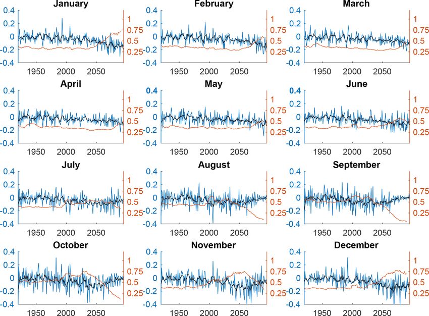
114                                       J. R. Mioduszewski et al.: Past and future interannual variability in Arctic sea ice

tic stakeholders (Ridley et al., 2016). Nonetheless, navigation     the early 20th century through the entire 21st century and
through the Arctic has already increased in frequency as a re-      find very different behavior across the four seasons. These
sult of this decline (Melia et al., 2016; Eguíluz et al., 2016),    monthly differences are societally important because marine
and even more trade routes associated with the increased ice-       access to the Arctic will likely expand beyond late sum-
free season are expected throughout the 21st century (Ak-           mer as the ice pack shrinks. Second, we detail how inter-
senov et al., 2015; Stephenson et al., 2013).                       annual sea ice area variability changes as the ice pack re-
   As the Arctic sea ice pack thins and retreats, multiyear ice     treats, and we link enhanced future variability to optimal
is being lost and there is consequently a larger proportion of      ice thicknesses and to the various thermodynamic and dy-
seasonal thin first-year ice (Kwok et al., 2010; Maykut, 1978;      namic processes that control ice area variability. We analyze
Holland et al., 2006). Overall thinner ice may result in an ice     a large 40-member ensemble from a single global climate
pack that exhibits greater interannual variability (Maslanik        model (GCM), which allows us to isolate internal variabil-
et al., 2007b; Goosse et al., 2009; Notz, 2009; Kay et al.,         ity, which is otherwise muddled with inter-model variability
2011; Holland and Stroeve, 2011; Döscher and Koenigk,               in multi-model comparisons. This allows us to test the hy-
2013), at least partially due to enhanced ice growth and melt       pothesis that interannual Arctic sea ice cover variability will
(Maykut, 1978; Holland et al., 2006; Bathiany et al., 2016).        increase throughout the year in the future as the ice pack di-
Decreased ice thickness promotes amplification of a positive        minishes.
ice–albedo feedback, which can magnify sea ice anomalies
(Grenfell and Maykut, 1977; Maykut, 1982; Ebert and Curry,
1993; Perovich et al., 2007; Hunke and Lipscomb, 2010),             2   Data and methods
and thin ice is more vulnerable to anomalous atmospheric
forcing and oceanic transport due to the smaller amount of          Ice thickness, concentration, and area were obtained from
energy required to completely melt the ice (Maslanik et al.,        simulations of the Community Earth System Model Large
1996; Zhao et al., 2018) and deform the ice dynamically (Hi-        Ensemble Project (CESM-LE). Ice concentration refers to
bler, 1979). For example, pulse-like increases in oceanic heat      the percentage of a given grid cell that is covered by ice,
transport can trigger abrupt ice-loss events in sufficiently thin   while ice area in this study refers specifically to this percent
ice (Woodgate et al., 2012).                                        coverage multiplied by the area of the grid cell, yielding a to-
   Changes in the interannual variability in sea ice cover-         tal Arctic ice-covered area. The CESM-LE was designed to
age have been studied only in a limited capacity, likely be-        enable an assessment of projected change in the climate sys-
cause they are only beginning to become visible in Septem-          tem while incorporating a wide range of internal climate vari-
ber in the present day. Both Goosse et al. (2009) and Swart et      ability (Kay et al., 2015). It consists of 40 ensemble mem-
al. (2015; their Fig. S6 in the Supplement) reported that max-      bers simulating the period 1920–2100 under historical and
imum ice area variability during September occurs once the          projected (RCP8.5 emissions scenario only) external forcing.
mean ice extent declines to 3–4 million km2 . This increased        The ensemble members are produced by introducing a small,
variability may occur due to increased prevalence of RILEs          random round-off level difference in the initial air tempera-
and periods of rapid recovery during this timeframe (Döscher        ture field for each member. This then generates a consequent
and Koenigk, 2013). The thickness distribution during these         ensemble spread that is purely due to simulated internal cli-
periods skews toward thinner ice, which is conducive to both        mate variability. A full description of the CESM-LE is given
rapid ice loss and rapid recovery processes (Tietsche et al.,       in Kay et al. (2015), and similar ensembles using the weaker
2011; Döscher and Koenigk, 2013). Holland et al. (2008)             RCP4.5 and RCP2.6 scenarios can be found in Sanderson et
considered a critical ice thickness that can serve as a precur-     al. (2017, 2018).
sor to RILEs but found it more likely that intrinsic variabil-         Another data set used in the current study is the model sim-
ity played the primary role in the particular RILEs that were       ulations from the Coupled Model Intercomparison Project
studied. More recently, Massonnet et al. (2018) analyzed the        Phase 5 (CMIP5). Although more than 40 models submitted
projected variability in sea ice volume and its projected future    their simulation results to the Program for Climate Model Di-
change in the CMIP5 ensemble, which suggested a mono-               agnosis and Intercomparison (PCMDI), only 12 of them sim-
tonic future decrease. The corresponding variability in sea         ulated the Arctic sea ice extent of both the monthly means
ice area was investigated by Olonscheck and Notz (2017),            (each individual month) and the magnitude of the seasonal
but their analysis was much coarser temporally and season-          cycle (March minus September sea-ice extent) within 20 %
ally than our study, in that it only compared changes between       error when compared with observations (Wang and Over-
two discrete time periods (the historical 1850–2005 period          land, 2012, 2015). Therefore, we used only these 12 mod-
vs. the future 2006–2100 interval) and was further restricted       els identified by Wang and Overland (2015) in this study:
to the summer and winter seasons.                                   ACCESS1.0, ACCESS1.3, CCSM4, CESM1(CAM5.1), EC-
   Building on these previous studies, our paper has two            EARTH, HadGEM2-AO, HadGEM2-CC, HadGEM2-ES,
novel aspects. First, we analyze the transient interannual          MIROC-ESM, MIROC-ESM-CHEM, MPI-ESM-LR, and
variability in sea ice area over the course of the year from        MPI-ESM-MR. Among the 12 models, half of them use the

The Cryosphere, 13, 113–124, 2019                                                        www.the-cryosphere.net/13/113/2019/
J. R. Mioduszewski et al.: Past and future interannual variability in Arctic sea ice 115
same sea ice model as CESM-LE (CICE; Hunke and Lip- each month, as found in Massonnet et al. (2012), but good
scomb, 2010) or a variation of it. If a GCM provided mul- agreement that variability increases in this timeframe.
tiple ensemble members, we only kept up to five realiza- The analysis of ice area variability in Figs. 2 and 3 follows
tions, so that the total ensemble numbers are close to that that of Goosse et al. (2009) and Swart et al. (2015), but we
used in CESM-LE. There is a total of 33 ensemble mem- extend their findings for September to all months and con-
bers from these 12 models in the RCP8.5 emissions scenario. firm that the variability in ice area is maximized as its total
Sea ice area, rather than ice extent, is computed from these basin area decline is well underway in both CESM-LE en-
12 CMIP5 models to be consistent with CESM-LE results. sembles and across CMIP5 models. A direct relationship be-
One of our primary analysis data sets is the time series of tween the rate of sea ice retreat and the magnitude of variabil-
monthly ice variables. The ensemble mean of all variables ity is evident in nearly all months in CESM-LE and CMIP5:
is taken after the statistics are calculated for each ensemble the standard deviation is generally highest when ice declines
member. The 1-year differences in ice area are calculated for the fastest (Figs. 1, 2 and S1, S2). Furthermore, the mag-
each month separately to remove the confounding effect of nitude and timing of peak ice area variability in both sets
amplified variability resulting from a downward trend. Fi- of experiments differ greatly by season. The peak in mag-
nally, a 10-year running standard deviation is applied to the nitude in CESM-LE is most pronounced from November
time series of 1-year differences in monthly ice area, centered to January when the running standard deviation of ice area
on a given year. A value of 10 years was chosen to quantify exceeds 1 × 10⁶ km2 , while the lowest magnitudes occur in
variability over decadal-scale intervals and to provide an ad- April and May, when the downward trend in ice area does
equate number of years for a standard deviation calculation. not peak prior to 2100 (Fig. 2). Near the end of the 21st cen-
The timing and magnitude of variability is generally insensi- tury, the running standard deviation also shows an increase in
tive to the standard deviation window, however, and whether the CMIP5 ensembles from December to June (Fig. 3), very
the 1-year difference in ice area or its raw time series is used. similar behavior to that displayed by CESM-LE. However,
the magnitude of the increase in the running standard devi-
ation in the CMIP5 ensemble mean is smaller than that in
3 Results CESM-LE. This is not surprising, as the timing of ice retreat
varies among models, so averaging them will smooth out the
3.1 Sea ice area and its variability possible signals. The CMIP5 models therefore provide addi-
tional evidence that increased variability is associated with
Sea ice area in the CESM-LE is projected to decline in all decreasing sea ice coverage.
months in the 21st century, proceeding in three phases: a
fairly stable regime of extensive coverage in the 20th cen- 3.2 Relationship between ice area variability and
tury, then a decline, followed by virtually no ice remaining thickness
in summer and autumn months (Fig. 1). Sea ice area variabil-
ity follows an analogous three-phase progression in months Because increasing future concentrations of thin ice are
spanning midsummer to early winter (Fig. 2). For example, likely a primary factor in increased ice area variability, we
in September this includes a period of modest variability dur- next consider the relationship between ice thickness and ice
ing the 20th century, then a distinct variability peak in the late area variability in CESM-LE. This is performed by correlat-
2020s and 2030s that coincides with the maximum rate of ice ing the standard deviation of basin-wide ice area (Fig. 2) with
retreat, and finally negligible variability in the late 21st cen- the total area of grid cells with mean ice thickness within
tury as the Arctic reaches near-ice-free conditions (Fig. 2). a given range for an aggregation of all years and ensem-
The first two phases of this progression in variability occur ble members, binned at 0.05 m intervals (Fig. 4). The 20th
for months in late winter to early summer (January–June), century data are omitted because both variables are largely
and suppressed variability would likely emerge beyond the stationary for this period. There is a large difference in the
end of the century, assuming that ice cover in these months maximum correlation coefficient across seasons, but in most
would continue to retreat. The maximum rate of ice retreat months it peaks between r = 0.6 and r = 0.8. This peak is
(negative values of the derivative) occurs at a different time associated with the thinnest ice of 0.1 to 0.2 m from October
in the 21st century in each month, occurring presently in to January, indicating that the greatest year-to-year variabil-
September but not until the end of the century in spring. ity in basin-wide ice area in these months occurs when there
The same relationship between ice area and its variability is the greatest coverage of thin sea ice between 0.1 and 0.2 m
is maintained across CMIP5 models, though with more noise thickness. There is a broad peak in the correlation coefficient
resulting from the aggregation of many different models between 0.25 and 0.40 m in August and September, while
rather than ensemble members from a single model (Fig. 3). July peaks near 0.45 m thickness but with a weaker maxi-
This is most notable in the sea ice area (1-year difference) mum correlation coefficient (r = 0.6). In June, r = 0.6 for
time series (Fig. 3, blue), indicating that there is consider- most ice thicknesses below 0.8 m, and there is only a weak
able spread in when and how the downward trend proceeds correlation between these variables in April and May.
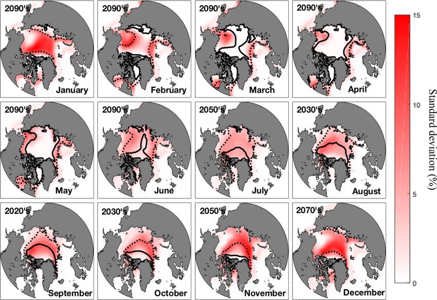
www.the-cryosphere.net/13/113/2019/ The Cryosphere, 13, 113–124, 2019116 J. R. Mioduszewski et al.: Past and future interannual variability in Arctic sea ice Figure 1. The CESM-LE ensemble mean time series of monthly sea ice area (km2 × 106 ). Figure 2. The CESM-LE ensemble mean of the 1-year differences in sea ice area (blue; million km2 ) with their 5-year running mean overlaid (black) and the running standard deviation of the interannual change in sea ice area (gold; million km2 ). The Cryosphere, 13, 113–124, 2019 www.the-cryosphere.net/13/113/2019/
J. R. Mioduszewski et al.: Past and future interannual variability in Arctic sea ice                                                  117

Figure 3. As in Fig. 2, but for the ensemble mean from 12 CMIP5 models’ sea ice area.

Figure 4. Monthly correlation coefficient (r) of the 2000–2100 10-year running standard deviation of 1-year difference in sea ice area with
mean grid cell ice thickness binned every 0.05 m of thickness.

   The analysis in Fig. 4 allows us to identify a common                throughout the basin by calculating the total area of ice that
range of ice thicknesses when ice area variability generally            falls within that range. The time-transgressive nature of when
peaks regardless of the month, which we approximate as 0.2              the peak in thin ice cover occurs (earliest in September, latest
to 0.6 m. We next track the temporal evolution of this thin ice         in winter–spring) is consistent with the corresponding timing

www.the-cryosphere.net/13/113/2019/                                                              The Cryosphere, 13, 113–124, 2019
118                                      J. R. Mioduszewski et al.: Past and future interannual variability in Arctic sea ice

Figure 5. The CESM-LE ensemble mean of the 10-year running standard deviation of 1-year difference in sea ice area from Fig. 1 (gold;
million km2 ) and the ensemble mean total area of grid cells with mean ice thickness between 0.2 and 0.6 m (blue; million km2 ).

of the peak future sea ice area variability, suggesting that the     to the boundary of maximum variability in ice coverage in
emergence of a sufficiently thin and contracted ice pack is          most months, which is consistent with results from Figs. 4
a primary factor for enhanced ice cover variability (Fig. 5).        and 5. This demonstrates the first-order relationship between
Both curves match each other in shape, with a steady state           thin ice and the variability in interannual ice coverage within
early, increasing to a peak and dropping to zero as the Arc-         a given region.
tic becomes ice free. The exception is in the spring and early
summer when neither increases until the end of the 21st cen-         3.3   Ice concentration tendency
tury, when ice begins to decline more rapidly. The two curves
are largely in phase as well, with one preceding the other by        The strong relationship between thin ice coverage and high
no more than 10–20 years in July, August, and November–              concentration variability occurs primarily due to the differing
January. The phase difference is due to the chosen range of          underlying mechanisms controlling ice concentration vari-
ice thicknesses, since the best relationship varies by month         ability at a given time, namely whether ice is expanding or
(Fig. 4). The two curves are in phase from August to October         retreating. To illustrate this, we chose two months representa-
(Fig. 5) when the 0.2 to 0.6 m range approximates the best           tive of these processes, September and December, to conduct
relationship between thickness and variability (Fig. 4). How-        an in-depth analysis of the physical mechanisms involved in
ever, ice area variability maximizes after the peak in 0.2–          the time difference in the two curves in Fig. 5. September is
0.6 m thickness area in November–January because variabil-           the end of the melt season, and therefore the ice concentra-
ity is more highly correlated with ice slightly thinner than         tion over the entire basin in this month reflects the cumulative
0.2 m in these months (Figs. 4, 5).                                  impact of melt processes throughout the summer. By con-
   There are also notable seasonal differences in the spatial        trast, December is a time of ice growth, particularly in the
pattern of variability during the decade when variability in         future, and thus the ice concentration in this month is largely
ice concentration peaks in CESM-LE (Fig. 6). The largest             regulated by cumulative growth processes during autumn.
fluctuations occur in a horseshoe-shaped pattern across the          Using available model output, we calculate the ice concentra-
Arctic Ocean in autumn, but they are restricted to the bound-        tion tendency (% day−1 ) from thermodynamics and dynam-
aries of the Atlantic and Pacific oceans in late winter and          ics in the regions where the decadal standard deviation of
spring. The result is a larger area of high variability in the       ice concentration exceeds 30 % within the grid cell (Fig. S3)
second half of the year and into January. The mean 0.2 m             to evaluate the mean ice budget. These regions of maximum
(dotted) and 0.6 m (solid) ice thickness contours are over-          variability in September and December closely match those
laid for reference (Fig. 6). The contours correspond closely         in Fig. 6, though the magnitude is smaller in Fig. 6 due to the

The Cryosphere, 13, 113–124, 2019                                                          www.the-cryosphere.net/13/113/2019/
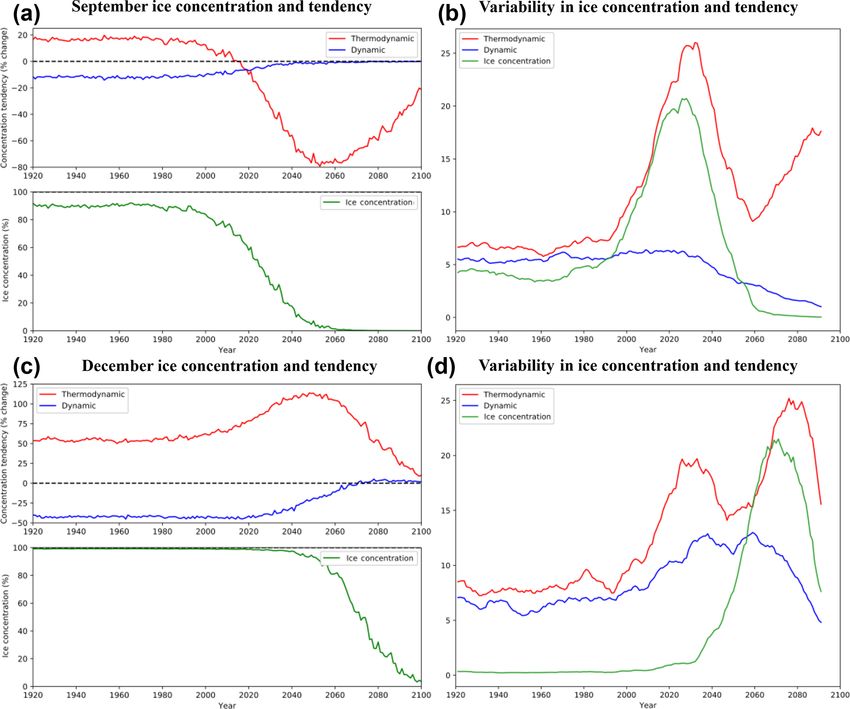
J. R. Mioduszewski et al.: Past and future interannual variability in Arctic sea ice                                              119

Figure 6. Monthly ensemble average in CESM-LE of the 10-year running standard deviation of ice concentration (%) in the decade when
ice area variability is at a maximum. Mean 0.2 and 0.6 m ice thicknesses are indicated by the dotted and solid contours, respectively.

standard deviation being a decadal mean. The daily change            first-order forcing explaining future ice concentration vari-
in ice concentration is a function of dynamic contributions          ability, particularly given that the magnitude of the dynamic
(ice import–export and ridging), thermodynamic melt pro-             contribution approaches zero by the 2020s when ice cover
cesses (the sum of top, bottom, and lateral), and thermody-          is rapidly diminishing. As shown in Fig. 7b, the peak inter-
namic growth (frazil and congelation). Because antecedent            annual variability in the thermodynamic term (red curve) is
conditions of the ice pack can be an important factor for de-        indeed several times larger than peak variability in the dy-
termining ice concentration in the month of interest, we sum         namic term (blue curve), and the variability in the thermody-
these terms over the preceding months (July–September or             namic term maximizes during the late 2020s in phase with
October–December) and report the net 3-month change in               the variability in the ice concentration (green curve) when
ice concentration resulting from each component.                     the thermodynamic term is declining most rapidly in Fig. 7a.
   The most interannually variable ice cover during Septem-          The variability likely also reflects the influence of the surface
ber occurs primarily in the 2020s and is centered across the         albedo feedback in amplifying summer ice area variations.
central Arctic (Fig. S3), though this region displays net ice        There is a secondary rise in the variability in the thermody-
expansion in July–September in the 20th century (Fig. 7a)            namic term after 2060 (Fig. 7b), coinciding with its rapid rise
due to rapid ice growth in September. Thermodynamic pro-             toward zero in Fig. 7a, but ice coverage by this point is con-
cesses dominate over dynamics and are of opposing sign dur-          fined to a diminishing area.
ing the 20th century, and thermodynamic processes add an                From the 20th century well into the 21st century, ice
average of 20 % to the ice concentration of each grid cell in        growth occurs in the October–December period in a simi-
the region by the end of September, compared with a loss             lar region of maximum interannual variability as September,
of only 10 % from dynamical processes (Fig. 7a). Ice growth          except slightly equatorward (Fig. S3). Ice export plays a rel-
diminishes and melt processes accelerate in the early to mid-        atively larger role in the regions of interest in December than
21st century when the melt processes reduce ice concentra-           in September (Fig. 7c). However, the thermodynamic ten-
tion by more than 75 % and the dynamic processes essen-              dency is still the dominant term controlling ice concentration
tially disappear with less ice to export (Fig. 7a). After 2060,      within this region of maximum interannual variability, and
September ice-free conditions occur, and the thermodynamic           this term increases in the early to mid-21st century to a total
term becomes less negative due to reduced areal coverage of          of nearly 120 %, some of which is offset by ice export that
ice in June and hence less ice area to melt over the summer          contributes to a 40 % decrease in mean ice concentration in
(Fig. 7a).                                                           the 20th and early 21st centuries (Fig. 7c). The increased net
   Because thermodynamic processes dominate in control-              ice growth occurs at this time primarily because there is more
ling ice concentration in the future, they should also be the        initial open water on which frazil ice can form.

www.the-cryosphere.net/13/113/2019/                                                           The Cryosphere, 13, 113–124, 2019
120                                      J. R. Mioduszewski et al.: Past and future interannual variability in Arctic sea ice

Figure 7. Time series of ensemble-mean (a) September ice concentration (%) and July–September averaged concentration tendency
(% day−1 ) from dynamics and thermodynamics, and (b) the 10-year running standard deviation of the interannual difference in ice con-
centration (%), and July–September ice concentration tendency from dynamics and thermodynamics (% day−1 ). The same information is
presented in panels (c) and (d) for December concentration and October–December ice concentration tendency terms.

   Figure 7d shows that the standard deviation of Decem-             in the 2050s and 2060s (Fig. 7c). This is reflected in the peak
ber ice concentration (green curve) peaks around 2070 and            in variability in the thermodynamic tendency (red curve) ap-
is accompanied by a peak in the variability in the thermo-           proximately corresponding to the timing of the peak in the
dynamic tendency (red curve) of more than double the mag-            ice area variability (green curve) in 2070 (Fig. 7d). The co-
nitude of its dynamic tendency (blue curve). A smaller first         incidence in their peak variability is similar to that in Fig. 7b
peak in thermodynamic tendency occurs in the 2020s, when             and underscores the dominance of thermodynamics over dy-
ice growth in this region increases due to increased frazil          namics in regulating the variability in ice area.
growth as this region’s waters become more open on average
in October. This initial peak may be smaller due to the anti-
correlation between dynamic and thermodynamic tendency,              4   Discussion and conclusions
which reduces the effect of the latter. The rapid subsequent
decline in ice growth occurs as conditions become too warm           This study has assessed the behavior of interannual Arctic
for ice growth over much of the October–December period              sea ice area variability in the past and future, using a large set
                                                                     of independent realizations from CESM-LE and simulations

The Cryosphere, 13, 113–124, 2019                                                          www.the-cryosphere.net/13/113/2019/
J. R. Mioduszewski et al.: Past and future interannual variability in Arctic sea ice 121
from 12 models participating in CMIP5. The results demon- son (Figs. 4–5). The mean ice thickness in late summer
strate the complex, time-varying response of the ice pack as and autumn is close to 0.6 m when ice area variability is
it transitions from a relatively stable state during the 20th highest, but is 0.2 m or less for a grid cell average in the
century to a more volatile state. A few of our most important winter.
findings are summarized below. Increased ice area variability in summer and autumn is
1. Interannual variability in Arctic sea ice cover increases partly attributable to a higher efficiency of open wa-
(at least transiently) in all months in the future as sea ice ter formation with the thinning sea ice (Holland et
area and thickness decline, but there is a strong seasonal al., 2006; Massonnet et al., 2018) and the fact that
dependence. There is also a strong seasonal dependence smaller heating anomalies are required to completely
of the magnitude of the maximum ice area variability in melt through vast areas of the thin ice pack (Bitz and
the future, with the greatest magnitude occurring during Roe, 2004). We find that the total area of thin ice be-
autumn and winter and smallest during spring by the tween the range of 0.2 and 0.6 m is closely related to
time the simulation ends in 2100 (Figs. 2–3). The fu- how soon and how strongly the peak variability in basin-
ture peak in variability emerges soonest in late-summer wide ice area emerges, and this is primarily a function of
months and latest during spring months, and the magni- variability in ice area’s thermodynamic tendency. This
tude of this peak is positively correlated with the rate of result is consistent with a physical understanding of this
ice loss in every month. relationship since ice that is too thin tends to be sea-
sonal and melt off every year, whereas thick ice is more
It is possible that the seasonal differences in ice area likely to survive the melt season. Seasonal forecasting
variability are partially a construction of the geography of September sea ice coverage takes advantage of this
of the Arctic Basin, as evident in Fig. 6: when the ice concept, with the forecast skill improved when initializ-
margin is geographically constrained and unable to ex- ing ice thickness up to 8 months in advance (Chevallier
pand and contract due to a coastline early in the simula- and Salas-Melia, 2012; Day et al., 2014).
tion, there is a smaller area subject to high ice variabil-
In contrast, ice area variability in November–January
ity. This explanation was offered by Goosse et al. (2009)
arises primarily from interannual variability in ice
for the same relationship in summer ice area variability,
growth (as represented by December in Fig. 7c, d),
as well as by Eisenman (2010), to explain retreat rate
which is dependent on existing open water conditions
differences between summer and winter. In the future,
and temperature anomalies. The peak in ice area vari-
the ice in the central Arctic Ocean becomes thin enough
ability in these months also coincides with a slightly
to expand and contract extensively each season, lead-
lower mean ice thickness of 0.2 m, though it is unclear
ing to an increase in variability. Therefore, variability
whether that is due to this ice growth processes rather
could be considered to be limited particularly in the first
than melt processes at work during the winter.
phase of its time series (Fig. 2) by the inability of ice
to spread across a large open area. Support for this in- 3. Interannual variability in ice concentration is driven pri-
terpretation comes from our calculation of Eisenman’s marily by thermodynamic mechanisms, which are pri-
equivalent ice area applied to Fig. 1 (not shown), which marily comprised of either ice growth or ice melt de-
resulted in the largest absolute decline in sea ice during pending on the season. Despite being opposing pro-
the winter–spring months, though summer–autumn ice cesses, their magnitudes exceed those of dynamic ice
loss was still greater in relative terms. While useful for processes (Fig. 7).
approximating potential sea ice extent in the absence of
The thermodynamic tendency in ice concentration is
geographic constraints, equivalent ice area is still a the-
of much greater magnitude than its dynamic counter-
oretical construct; our purpose is to assess the variabil-
part at both the end of the melt season and start of the
ity in ice cover that actually exists. Furthermore, results
growth season, and the maximum interannual variabil-
from Figs. 4 and 5 suggest that the amount of thin ice
ity in the thermodynamic term is mostly in phase with
alone can explain the evolution of ice variability in ev-
that of ice concentration. The inverse relationship be-
ery month, though differences in the optimal ice thick-
tween ice area’s interannual variability and its interan-
ness by month may require a partial geographical expla-
nual rate of change (Figs. 1, 2, S1, S2) is also found
nation, in addition to one incorporating the components
between the thermodynamic tendency and its rate of
of the thermodynamic tendency of ice area from Fig. 7.
change (not shown, but inferred from Fig. 7). This is fur-
2. Ice needs to be sufficiently thin before areal variabil- ther evidence that ice area variability is primarily driven
ity maximizes, and in CESM-LE the optimal thick- by thermodynamic processes in the ice pack.
ness range is generally between 0.2 and 0.6 m but with The dominance of the thermodynamic tendency is un-
some seasonal dependence resulting from the ice melt surprising and has been established as the relatively
or ice growth processes that dominate in a given sea- more important set of processes controlling sea ice vari-
www.the-cryosphere.net/13/113/2019/ The Cryosphere, 13, 113–124, 2019122 J. R. Mioduszewski et al.: Past and future interannual variability in Arctic sea ice
ability, primarily via transport of midlatitude eddy heat Data availability. CESM LE data are publicly available at the
flux anomalies (Kelleher and Screen, 2018), anticyclone National Center for Atmospheric Research Climate Data Gate-
passage (Wernli and Papritz, 2018), and increased ocean way (https://www.earthsystemgrid.org/, last access: 12 May 2018).
heat transport (Li et al., 2018). However, the dynamic CMIP5 data are publicly available and hosted by Lawrence
contribution to changes in ice concentration can likely Livermore National Laboratory (https://esgf-node.llnl.gov/projects/
cmip5/, last access: 15 November 2017).
be substantial in the absence of regional and monthly
averaging, and numerous mechanisms have been de-
scribed that can generate increased ice transport. Recent
Supplement. The supplement related to this article is available
examples include divergent ice drift events connected
online at: https://doi.org/10.5194/tc-13-113-2019-supplement.
to anomalous circulation patterns (Zhao et al., 2018) as
well as the collapse of the Beaufort high (Petty, 2018;
Moore et al., 2018), both of which may become more Author contributions. JRM analyzed the CESM data and prepared
common in the future due to preconditioning of the ice the paper, MW provided CMIP5 data and guidance, SV assisted in
pack and further intrusion of midlatitude cyclones into paper preparation and revision, and MH and LL provided guidance
the Arctic. and edits.
This study offers a unique contribution by focusing on the
projected transient evolution of Arctic sea ice area variability Competing interests. The authors declare that they have no conflict
throughout the year, as characterized by its response to exter- of interest.
nal greenhouse forcing superimposed on short-term internal
variability. A recent study (Olonscheck and Notz, 2017) also
identified an overall increase in projected interannual vari- Acknowledgements. We thank the two anonymous reviewers for
ability in summertime sea ice area in CMIP5, but this conclu- their helpful comments. Support was provided by the NOAA
sion was not consistent across all models, possibly because Climate Program Office under Climate Variability and Pre-
the analysis did not incorporate the pronounced changes in dictability Program grant NA15OAR4310166. This project is
variability over time as the ice pack diminishes. Interestingly, partially funded by the Joint Institute for the Study of the Atmo-
another recent study (Massonnet et al., 2018) revealed that sphere and Ocean (JISAO) under NOAA Cooperative Agreement
CESM-LE simulates a future decrease in interannual vari- NA10OAR4320148, contribution number 2017-087, the Pacific
Marine Environmental Laboratory contribution number 4671. We
ability in sea ice volume, due to the dominance of the sea
would like to acknowledge high-performance computing support
ice thickness term. Contrary to the behavior of ice area vari- from Yellowstone (ark:/85065/d7wd3xhc) provided by NCAR’s
ability analyzed here, their analysis showed that interannual Computational and Information Systems Laboratory, sponsored by
variability in ice thickness consistently declines when the ice the National Science Foundation.
pack thins. This relationship is a robust thermodynamic con-
sequence of a strengthened “ice-formation efficiency”, in- Edited by: Dirk Notz
dicative of an enhanced stabilizing ice thickness–ice growth Reviewed by: Dirk Olonscheck and one anonymous referee
feedback (Notz and Bitz, 2017) caused by greater wintertime
vertical ice growth following summers with pronounced ice
thinning. Therefore, it is important to distinguish which term
(area or thickness) is being considered when assessing future References
changes in the variability in the ice pack.
Increased interannual variability in sea ice area in the Aksenov, Y., Popova, E. E., Yool, A., Nurser, J. G., Williams,
T. D., Bertino, L., and Bergh, J.: On the future nav-
CESM Large Ensemble as sea ice declines most rapidly is
igability of Arctic sea routes: High-resolution projections
an important result that needs to be accounted for as the ice- of the Arctic Ocean and sea ice, Mar. Policy, 75, 1–18,
free season expands and the timing of maximum variability https://doi.org/10.1016/j.marpol.2015.12.027, 2015.
shifts from September. We also confirm that this relationship Bathiany, S., van der Bolt, B., Williamson, M. S., Lenton, T. M.,
is maintained across CMIP5 models, suggesting that the re- Scheffer, M., van Nes, E. H., and Notz, D.: Statistical indica-
sponsible mechanisms reported here may apply more gen- tors of Arctic sea-ice stability – prospects and limitations, The
erally. These results have important implications for marine Cryosphere, 10, 1631–1645, https://doi.org/10.5194/tc-10-1631-
navigation going forward, indicating that the otherwise aus- 2016, 2016.
picious transition to diminished sea ice in every month may Bitz, C. M. and Roe, G. H.: A mechanism for the high
be accompanied by a confounding increase in interannual rate of sea ice thinning in the Arctic Ocean, J. Cli-
variability in the ice cover before the ice disappears com- mate, 17, 3623–3632, https://doi.org/10.1175/1520-
0442(2004)0172.0.CO;2, 2004.
pletely.
Cavalieri, D. J. and Parkinson, C. L.: Arctic sea ice vari-
ability and trends, 1979–2010, The Cryosphere, 6, 881–889,
https://doi.org/10.5194/tc-6-881-2012, 2012.
The Cryosphere, 13, 113–124, 2019 www.the-cryosphere.net/13/113/2019/J. R. Mioduszewski et al.: Past and future interannual variability in Arctic sea ice 123 Chevallier, M. and Salas-Melia, D.: The Role of Sea Ice Thickness jections, mechanisms, and implications, edited by: DeWeaver, Distribution in the Arctic Sea Ice Potential Predictability: A Di- E. T., Bitz, C. M., and Tremblay, L. M., Geophysical Mono- agnostic Approach with a Coupled GCM, J. Climate, 25, 3025– graph Series, American Geophysical Union, Washington, 133– 3038, 2012. 150, https://doi.org/10.1029/180GM10, 2008. Collins, M., Knutti, R., Arblaster, J., Dufresne, J.-L., Fichefet, T., Hunke, E. C. and Lipscomb, W. H.: CICE: the Los Alamos Sea Ice Friedlingstein, P., Gao, X., Gutowski, Jr, W. J., Johns, T., Krin- Model Documentation and Software User’s Manual Version 4.1 ner, G., Shongwe, M., Tebaldi, C., Weaver, A. J., and Wehner, LA-CC-06-012, T-3 Fluid Dynamics Group, Los Alamos Na- M.: Long-term Climate Change: Projections, Commitments and tional Laboratory, Los Alamos, NM, USA, 2010. Irreversibility, in: Climate Change 2013: The Physical Science Jahn, A., Kay, J. E., Holland, M. M., and Hall, D. M.: How pre- Basis, Contribution of Working Group I to the Fifth Assessment dictable is the timing of a summer ice-free Arctic?, Geophys. Report of the Intergovernmental Panel on Climate Change, edited Res. Lett., 43, 1–8, https://doi.org/10.1002/2016GL070067, by: Stocker, T. F., Qin, D., Plattner, G.-K., Tignor, M., Allen, S. 2016. K., Boschung, J., Nauels, A., Xia, Y., Bex, V., and Midgley, P., Kay, J. E., Holland, M. M., and Jahn, A.: Inter-annual Cambridge University Press, Cambridge, UK and New York, NY, to multi-decadal Arctic sea ice extent trends in a USA, 12, 1029–1136, 2013. warming world, Geophys. Res. Lett., 38, L15708, Comiso, J. C., Meier, W. N., and Gersten, R.: Variabil- https://doi.org/10.1029/2011GL048008, 2011. ity and trends in the Arctic Sea ice cover: Results from Kay, J. E., Deser, C., Phillips, A., Mai, A., Hannay, C., Strand, different techniques, J. Geophys. Res.-Oceans, 122, 1–22, G., Arblaster, J. M., Bates, S. C., Danabasoglu, G., Edwards, https://doi.org/10.1002/2017JC012768, 2017. J., Holland, M., Kushner, P., Lamarque, J.-F., Lawrence, D., Day, J. J., Tietsche, S., and Hawkins, E.: Pan-Arctic and regional sea Lindsay, K., Middleton, A., Munoz, E., Neale, R., Oleson, K., ice predictability: Initialization month dependence, J. Climate, Polvani, L., and Vertenstein, M.: The Community Earth Sys- 27, 4371–4390, 2014. tem Model (CESM) Large Ensemble Project: A Community Re- Ding, Q., Schweiger, A., L’Heureux, M., Battisti, D. S., source for Studying Climate Change in the Presence of Inter- Po-Chedley, S., Johnson, N. C., Blanchard-Wrigglesworth, nal Climate Variability, B. Am. Meteorol. Soc., 96, 1333–1349, E., Harnos, K., Zhang, Q., and Eastman, R.: Influence https://doi.org/10.1175/BAMS-D-13-00255.1, 2015. of high-latitude atmospheric circulation changes on sum- Kelleher, M. and Screen, J.: Atmospheric precursors of and re- mertime Arctic sea ice, Nat. Clim. Change, 7, 289–295, sponse to anomalous Arctic sea ice in CMIP5 models, Adv. At- https://doi.org/10.1038/nclimate3241, 2017. mos. Sci., 35, 27–37, https://doi.org/10.1007/s00376-017-7039- Döscher, R. and Koenigk, T.: Arctic rapid sea ice loss events in re- 9, 2018. gional coupled climate scenario experiments, Ocean Sci., 9, 217– Kwok, R. and Rothrock, D. A.: Decline in Arctic sea ice thickness 248, https://doi.org/10.5194/os-9-217-2013, 2013. from submarine and ICESat records: 1958–2008, Geophys. Res. Ebert, E. E. and Curry, J. A.: An intermediate one-dimensional Lett., 36, L15501, https://doi.org/10.1029/2009GL039035, 2009. thermodynamic sea ice model for investigating ice- Kwok, R., Cunningham, G. F., Wensnahan, M., Rigor, I., Zwally, atmosphere interactions, J. Geophys. Res., 98, 10085–10109, H. J., and Yi, D.: Thinning and volume loss of the Arctic Ocean https://doi.org/10.1029/93JC00656, 1993. sea ice cover: 2003–2008, J. Geophys. Res.-Oceans, 114, 2003– Eguíluz, V. M., Fernández-Gracia, J., Irigoien, X., and Duarte, C. 2008, https://doi.org/10.1029/2009JC005312, 2009. M.: A quantitative assessment of Arctic shipping in 2010–2014, Kwok, R., Pederse, L. T., Gudmandsen, P., and Pang, S. S.: Large Sci. Rep., 6, 30682, https://doi.org/10.1038/srep30682, 2016. sea ice outflow into the Nares strait in 2007, Geophys. Res. Lett, Eisenman, I.: Geographic muting of changes in the Arc- 37, L03502, https://doi.org/10.1029/2009GL041872, 2010. tic sea ice cover, Geophys. Res. Lett., 371, L16501, Labe, Z., Magnusdottir, G., and Stern, H.: Variability of Arctic Sea https://doi.org/10.1029/2010GL043741, 2010. Ice Thickness Using PIOMAS and the CESM Large Ensemble, Goosse, H., Arzel., O., Bitz, C. M., de Montety, A., and Van- J. Climate, 31, 3233–3247, https://doi.org/10.1175/JCLI-D-17- coppenolle, M.: Increased variability of the Arctic summer ice 0436.1, 2018. extent in a warmer climate, Geophys. Res. Lett., 36, L23702, Lang, A., Yang, S., and Kaas, E.: Sea ice thickness and re- https://doi.org/10.1029/2009GL040546, 2009. cent Arctic warming, Geophys. Res. Lett., 44, 409–418, Grenfell, T. C. and Maykut, G. A.: The optical properties of https://doi.org/10.1002/2016GL071274, 2017. ice and snow in the Arctic Basin, J. Glaciol., 18, 445–463, Li, D., Zhang, R., and Knutson, T.: Comparison of Mecha- https://doi.org/10.3189/S0022143000021122, 1977. nisms for Low-Frequency Variability of Summer Arctic Sea Hibler, W. D.: A dynamic thermodynamic sea ice model, J. Phys. Ice in Three Coupled Models, J. Climate, 31, 1205–1226, Oceanogr., 9, 815–846, 1979. https://doi.org/10.1175/JCLI-D-16-0617.1, 2018. Holland, M. M. and Stroeve, J.: Changing seasonal sea ice predictor Maslanik, J. A., Serreze, M. C., and Barry, R. G.: Recent de- relationships in a changing Arctic climate, Geophys. Res. Lett., creases in Arctic summer ice cover and linkages to atmo- 38, L18501, https://doi.org/10.1029/2011GL049303, 2011. spheric circulation anomalies, Geophys. Res. Lett., 23, 1677– Holland, M. M., Bitz, C. M., and Tremblay, B.: Future abrupt re- 1680, https://doi.org/10.1029/96GL01426, 1996. ductions in the summer Arctic sea ice, Geophys. Res. Lett., 33, Maslanik, J. A., Drobot, S., Fowler, C., Emery, R., and Barry, R.: 1–5, https://doi.org/10.1029/2006GL028024, 2006. On the Arctic climate paradox and the continuing role of atmo- Holland, M. M., Bitz, C. M., Tremblay, B., and Bailey, D. A.: spheric circulation in affecting sea ice conditions, Geophys. Res. The role of natural versus forced change in future rapid sum- Lett., 34, 2–5, https://doi.org/10.1029/2006GL028269, 2007a. mer Arctic ice loss. Arctic sea ice decline: Observations, pro- www.the-cryosphere.net/13/113/2019/ The Cryosphere, 13, 113–124, 2019
124                                           J. R. Mioduszewski et al.: Past and future interannual variability in Arctic sea ice

Maslanik, J. A., Fowler, C., Strove, J., Drobot, S., Zwally, J., Yi, D.,   Ridley, J. K., Wood, R. A., Keen, A. B., Blockley, E., and
  and Emery, W.: A younger, thinner Arctic ice cover: Increased               Lowe, J. A.: Brief Communication: Does it matter exactly when
  potential for rapid, extensive sea-ice loss, Geophys. Res. Lett.,           the Arctic will become ice-free?, The Cryosphere Discuss.,
  34, 2004–2008, https://doi.org/10.1029/2007GL032043, 2007b.                 https://doi.org/10.5194/tc-2016-28, in review, 2016.
Maslanik, J. A., Stroeve, J., Fowler, C., and Emery, W.: Distribution      Sanderson, B. M., Xu, Y., Tebaldi, C., Wehner, M., O’Neill, B.,
  and trends in Arctic sea ice age through spring 2011, Geophys.              Jahn, A., Pendergrass, A. G., Lehner, F., Strand, W. G., Lin, L.,
  Res. Lett., 38, 2–7, https://doi.org/10.1029/2011GL047735,                  Knutti, R., and Lamarque, J. F.: Community climate simulations
  2011.                                                                       to assess avoided impacts in 1.5 and 2 ◦ C futures, Earth Syst. Dy-
Massonnet, F., Fichefet, T., Goosse, H., Bitz, C. M., Philippon-              nam., 8, 827–847, https://doi.org/10.5194/esd-8-827-2017, 2017.
  Berthier, G., Holland, M. M., and Barriat, P.-Y.: Constraining           Sanderson, B. M., Oleson, K. W., Strand, W. G., Lehner, F., and
  projections of summer Arctic sea ice, The Cryosphere, 6, 1383–              O’Neill, B. C.: A new ensemble of GCM simulations to as-
  1394, https://doi.org/10.5194/tc-6-1383-2012, 2012.                         sess avoided impacts in a climate mitigation scenario, Climatic
Massonnet, F., Vancoppenolle, M., Goosse, H., Docquier, D.,                   Change, 146, 303–318, 2018.
  Fifechet, T., and Blanchard-Wrigglesworth, E.: Arctic sea-ice            Serreze, M. C. and Stroeve, J. C.: Arctic sea ice trends, variability
  change tied to its mean state through thermodynamic processes,              and implications for seasonal ice forecasting, Philos. T. Roy. Soc.
  Nat. Clim. Change, 8, 599–603, 2018.                                        A, 373, 20140159, https://doi.org/10.1098/rsta.2014.0159, 2015.
Maykut, G. A.: Energy exchange over young sea ice in                       Stammerjohn, S., Massom, R., Rind, D., and Martinson, D.:
  the central Arctic, J. Geophys. Res., 83, 3646–3658,                        Regions of rapid sea ice change: An inter-hemispheric
  https://doi.org/10.1029/JC083iC07p03646, 1978.                              seasonal comparison, Geophys. Res. Lett., 39, L06501,
Maykut, G. A.: Large-scale heat exchange and ice produc-                      https://doi.org/10.1029/2012GL050874, 2012.
  tion in the central Arctic, J. Geophys. Res., 87, 7971–7984,             Stephenson, S. R., Smith, L. C., Brigham, L. W., and Agnew,
  https://doi.org/10.1029/JC087iC10p07971, 1982.                              J. A.: Projected 21st-century changes to Arctic marine access,
Melia, N., Haines, K., and Hawkins, E.: Sea ice decline and 21st              Climatic Change, 118, 885–899, https://doi.org/10.1007/s10584-
  century trans-Arctic shipping routes, Geophys. Res. Lett., 43,              012-0685-0, 2013.
  9720–9728, https://doi.org/10.1002/2016GL069315, 2016.                   Stroeve, J., Holland, M. M., Meier, W. Scambos, T., and Serreze,
Moore, G. W. K., Schweiger, A., Zhang, J., and Steele, M.:                    M.: Arctic sea ice decline: Faster than forecast, Geophys. Res.
  Collapse of the 2017 winter Beaufort High: A response                       Lett., 34, 1–5, https://doi.org/10.1029/2007GL029703, 2007.
  to thinning sea ice?, Geophys. Res. Lett., 45, 2860–2869,                Stroeve, J. C., Serreze, M. C., Holland, M. M., Kay, J. E., Maslanik,
  https://doi.org/10.1002/2017GL076446, 2018.                                 J., and Barrett, A. P.: The Arctic’s rapidly shrinking sea ice
Nghiem, S. V., Rigor, I. G., Perovich, D. K., Clemente-Colón,                 cover: a research synthesis, Climatic Change, 110, 1005–1027,
  P., Weatherly, J. W., and Neumann, G.: Rapid reduction                      https://doi.org/10.1007/s10584-011-0101-1, 2012.
  of Arctic perennial sea ice, Geophys. Res. Lett., 34, 1–6,               Swart, N. C., Fyfe, J. C., Hawkins, E., Kay, J. E., and Jahn, A.: In-
  https://doi.org/10.1029/2007GL031138, 2007.                                 fluence of internal variability on Arctic sea-ice trends, Nat. Clim.
Notz, D.: The future of ice sheets and sea ice: between reversible re-        Change, 5, 86–89, https://doi.org/10.1038/nclimate2483, 2015.
  treat and unstoppable loss, P. Natl. Acad. Sci. USA, 106, 20590–         Tietsche, S., Notz, D., Jungclaus, J. H., and Marotzke, J.: Recovery
  20595, https://doi.org/10.1073/pnas.0902356106, 2009.                       mechanisms of Arctic summer sea ice, Geophys. Res. Lett., 38,
Notz, D. and Bitz, C. M.: Sea ice in Earth system models, edited by:          1–4, https://doi.org/10.1029/2010GL045698, 2011.
  Thomas, D. N., John Wiley & Sons, Chichester, UK, 2017.                  Wang, M. and Overland, J. E.: A sea ice free summer Arc-
Notz, D. and Marotzke, J.: Observations reveal external driver                tic within 30 years?, Geophys. Res. Lett., 36, L07502,
  for Arctic sea-ice retreat, Geophys. Res. Lett., 39, 1–6,                   https://doi.org/10.1029/2009GL037820, 2009.
  https://doi.org/10.1029/2012GL051094, 2012.                              Wang, M. and Overland, J. E.: A sea ice free summer Arctic within
Notz, D. and Stroeve, J.: Observed Arctic sea-ice loss directly               30 years: An update from CMIP5 models, Geophys. Res. Lett.,
  follows anthropogenic CO2 emission, Science, 354, 747–750,                  39, L18501, https://doi.org/10.1029/2012GL052868, 2012.
  https://doi.org/10.1126/science.aag2345, 2016.                           Wang, M. and Overland, J. E.: Projected future duration of the sea-
Olonscheck, D. and Notz, D.: Consistently estimating internal vari-           ice-free season in the Alaskan Arctic, Prog. Oceanogr., 136, 50–
  ability from climate model simulations, J. Climate, 30, 9555–               59, https://doi.org/10.1016/j.pocean.2015.01.001, 2015.
  9573, 2017.                                                              Wernli, H. and Papritz, L.: Role of polar anticyclones and mid-
Overland, J. E. and Wang, M.: When will the summer Arctic                     latitude cyclones for Arctic summertime sea-ice melting, Nat.
  be nearly sea ice free?, Geophys. Res. Lett., 40, 2097–2101,                Geosci., 11, 108–113, https://doi.org/10.1038/s41561-017-0041-
  https://doi.org/10.1002/grl.50316, 2013.                                    0, 2018.
Perovich, D. K., Light, B., Eicken, H., Jones, K. F., Runci-               Woodgate, R. A., Weingartner, T. J., and Lindsay, R.: Observed
  man, K., and Nghiem, S. V.: Increasing solar heating of the                 increases in Bering Strait oceanic fluxes from the Pacific to
  Arctic Ocean and adjacent seas, 1979–2005: Attribution and                  the Arctic from 2001 to 2011 and their impacts on the Arc-
  role in the ice-albedo feedback, Geophys. Res. Lett., 34, 1–5,              tic Ocean water column, Geophys. Res. Lett., 39, L24603,
  https://doi.org/10.1029/2007GL031480, 2007.                                 https://doi.org/10.1029/2012GL054092, 2012.
Petty, A. A.: A possible link between winter Arctic sea ice decline        Zhao, J., Barber, D., Zhang, S., Yang, Q., Wang, X., and Xie,
  and a collapse of the Beaufort High?, Geophys. Res. Lett., 45,              H.: Record Low Sea-Ice Concentration in the Central Arc-
  2879–2882, https://doi.org/10.1002/2018GL077704, 2018.                      tic during Summer 2010, Adv. Atmos. Sci., 35, 106–115,
                                                                              https://doi.org/10.1007/s00376-017-7066-6, 2018.

The Cryosphere, 13, 113–124, 2019                                                                  www.the-cryosphere.net/13/113/2019/
You can also read