PORT PHILLIP BAY HABITAT MAP - HABITAT COMPLEX MODELLING (CBICS LEVEL 3) - MARINE AND COASTS
←
→
Page content transcription
If your browser does not render page correctly, please read the page content below

Port Phillip Bay Habitat Map
                                  Habitat Complex Modelling (CBiCS Level 3)

Marine Biodiversity Policy & Programs | Biodiversity Strategy and Knowledge | Biodiversity Division
                                           August 2021

                                            OFFICIAL
Acknowledgements

The Victorian Government proudly acknowledges Victoria’s Aboriginal communities and their rich culture and pays
respect to their Elders past and present. We recognise the intrinsic connection of the Kulin nation people to Nairm (Port
Phillip Bay) and its catchment, and we value their contribution in the management of land, water and the natural
landscape. We support the need for genuine partnerships with Aboriginal people and communities, to understand their
culture and connections to Country, and to better manage the Bay and its catchments. We embrace the spirit of
reconciliation, working towards the equality of outcomes and ensuring an equal voice. DELWP would like to acknowledge
and thank all individuals who provided data to support the outcomes of this work.

Authors
Dr. Tessa Mazor: Marine Spatial Analyst, Biodiversity Division, DELWP, tessa.mazor@delwp.vic.gov.au

Dr. Matt Edmunds: Australian Marine Ecology Pty Ltd, matt@marine-ecology.com.au

Dr. Adrian Flynn: Fathom Pacific Pty Ltd, adrian.flynn@fathompacific.com

Mr Lawrance Ferns: Marine Knowledge Manager, Biodiversity Division, DELWP, lawrance.ferns@delwp.vic.gov.au

Citation
Mazor, T., Edmunds, M., Flynn, A., Ferns, L. (2021) Port Phillip Bay Habitat Map. Habitat Complex Modelling (CBiCS
Level 3). The State of Victoria Department of Environment, Land, Water and Planning 2021.

ISBN 978-1-76105-690-1

Photo credit
Front cover: Marcia Riederer, DELWP

    Acknowledgment
    We acknowledge and respect Victorian Traditional Owners as the
    original custodians of Victoria's land and waters, their unique ability to
    care for Country and deep spiritual connection to it. We honour Elders
    past and present whose knowledge and wisdom has ensured the
    continuation of culture and traditional practices.
    We are committed to genuinely partner, and meaningfully engage, with
    Victoria's Traditional Owners and Aboriginal communities to support the
    protection of Country, the maintenance of spiritual and cultural practices and
    their broader aspirations in the 21st century and beyond.

© The State of Victoria Department of Environment, Land, Water and Planning 2021
                  This work is licensed under a Creative Commons Attribution 4.0 International licence. You are free to re-use the work
                  under that licence, on the condition that you credit the State of Victoria as author. The licence does not apply to any
                  images, photographs or branding, including the Victorian Coat of Arms, the Victorian Government logo and the
Department of Environment, Land, Water and Planning (DELWP) logo. To view a copy of this licence, visit
http://creativecommons.org/licenses/by/4.0/

Disclaimer
This publication may be of assistance to you but the State of Victoria and its employees do not guarantee that the publication is without
flaw of any kind or is wholly appropriate for your particular purposes and therefore disclaims all liability for any error, loss or other
consequence which may arise from you relying on any information in this publication.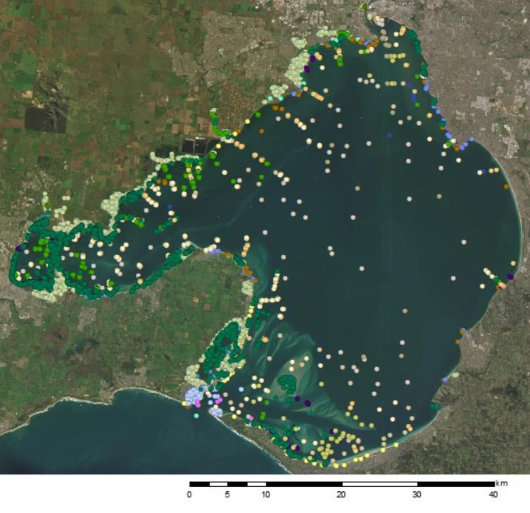
Port Phillip Bay Habitat Map
       Habitat maps represent                                  CoastKit
       communities of marine species                           CoastKit is a new DELWP online
       across Port Phillip Bay. They are                       platform for environmental managers
                                                               and researchers, that synthesises
       developed from observation
                                                               coastal scientific data and resources.
       records and environmental
       variables by applying machine
       learning methods to build
       predictive models that estimate
       their distribution. Habitat maps
       support the monitoring and
       management of marine
       biodiversity and health in the                          The spatial toolkit promotes
       region.                                                 standardised data classification for
                                                               collection, reporting, monitoring and

       Habitat Models                                          assessment across Victoria. CoastKit
                                                               support marine managers by
                                                               interactive tools that facilitate:
       Port Phillip Bay supports many different natural
       habitats. Along the foreshore are sandy beaches,         • Marine biotope distribution maps
       rocky intertidal reefs, mud flats, mangroves and         • Cumulative risk assessments
       saltmarshes. Habitats within the Bay include
                                                                • Marine environmental impact
       seagrass meadows, rocky reefs, sponge gardens
       and unvegetated soft sediments (sands and silt).           assessments
       Unvegetated soft sediments on the seafloor are           • Marine spatial planning
       home to a diverse array of invertebrates and micro-
                                                                • Ecsosytem modelling
       organisms that are critical in processing nitrogen
       and other nutrients. Seagrasses provide nurseries        • Marine habitat records
       for many fish and invertebrate species. Rocky reefs      • Ecosystem-based management
       provide hard substrate on which hundreds of                (EBM)
       species of seaweed grow. The Bay provides habitats
       for a diversity of marine plants and animals, many of   Ultimately, CoastKit unifies and
       which are endemic. They include hundreds of             disseminates relevant information to
       species of fish, molluscs, crustaceans, marine
       worms, jellyfish, sea anemones, algae (seaweeds),       improve the efficiency and
       sponges as well as seabirds, dolphins and little        effectiveness of decision making,
       penguins.                                               ensuring the future health and
       The health of Port Phillip Bay and its marine and       sustainability of Victoria’s unique
       coastal areas are vital for Victoria and its people,    marine and coastal assets.
       providing invaluable benefits ecologically,
       recreationally, and economically. Mapping the
       distribution and extent of marine habitats in the Bay
       helps achieve a better understanding of the             Further information about CoastKit
       ecosystem to monitor and maintain ecological            https://mapshare.vic.gov.au/coastkit/
       functions, ecosystem services and improve its
       overall health.

Port Phillip Bay Habitat Map                                                                 1
Habitat Complex Modelling (CBiCS Level 3)
                                               OFFICIAL
Habitat Classification System                                        Port Phillip Bay and offers a baseline for future data
                                                                     to build upon.
The habitat map uses the Combined Biotope
Classification Scheme (CBiCS) as developed and                       Ground-truth records
described by Edmunds and Flynn (2015, 2018;                          Ground-truth survey data provide the primary data to
2021). CBiCS has six, hierarchical classification                    build the habitat model. Field observations of
components; Level 1 – Environment, Level 2 –                         Victorian marine species and habitats are
Broad Habitat, Level 3 – Habitat Complex, Level 4 –                  categorised according to the CBiCS method to the
Biotope Complex, Level 5 – Biotope, Level 6 – Sub-                   lowest hierarchical level where possible. Records
biotope. The hierarchical design (Figure 1) is                       are combined from various sources including habitat
adopted directly from the United Kingdom’s Joint                     mapping, monitoring, impact assessments and
Nature Conservation Committee (JNCC) scheme                          historical ecological surveys. Across Port Phillip Bay
that is a proven system for classification. With some                9,683 ground-truth records have currently been
conversion, many of the actual classes from the                      categorised to level 3 - Habitat Complex across the
JNCC scheme that are mapped in Europe (e.g.,                         years 1969 to 2019 (Figure 2; Appendix Figure 1).
seaweed biotopes, mussel, worm, and other                            These records can be explored spatially using the
biogenic reefs) were imported directly into the                      ‘Biotope Atlas Tool’ in CoastKit.
Australian context (Edmunds et al. 2021). This
scheme also aligns with the terrestrial Ecological
Vegetation Class (EVC) system for recording
mangrove and saltmarsh biotopes.

                          Sub-
                         Biotope

                         Biotope

                     Biotope Complex

                     Habitat Complex

                      Broad Habitat

                   Environment (Marine)

Figure 1. Hierarchical classification system. CBiCS classification
components as outlined in Edmunds et al. (2021). Level 3 is
                                                                     Figure 2: Ground truth samples (9683 records at level 3) in Port
highlighted in yellow to indicate the level the resulting habitat
                                                                     Philip Bay, Victoria. Base map source: ESRI, (2021).
model was constructed.
                                                                     DigitalGlobe, GeoEye, i-cubed, USDA FSA, USGS, AEX,
                                                                     Getmapping, Aerogrid, IGN, IGP, swisstopo, and the GIS User
Building Habitat Models                                              Community. Created in ArcGIS (ESRI 2019).

Habitat models were built to predict habitat
distribution by applying machine learning tools which
                                                                     Environmental predictors
integrate ground truthed data and environmental
predictors. Level 3 Habitat Complex was selected                     Gridded data products that are at a high resolution
providing the lowest classification (Figure 1) with                  across Port Phillip Bay and that are considered
data availability to support a broad-scale model                     important predictors for marine habitats (i.e., biotope
across Port Phillip Bay. Previous mapping of Port                    related fauna and flora) were included in the model
Phillip Bay has provided insight into habitats across                (Table 1).
the region, with the latest map produced in 2016
(Edmunds & Flynn 2018). Since then, additional                       Environmental parameters were sourced from
benthic survey data and data on environmental                        different methods including lidar, multibeam, and
predictors has developed which increases the                         indexes calculated from the Digital Elevation Model
capacity to improve mapping outputs. This work                       (DEM), and mapped at a resolution of 2.5 metres
provides an updated broad-scale habitat map across                   (e.g., Figure 3). Predictor data were largely complete
                                                                     across the study region with few missing values (0-

2   Port Phillip Bay Habitat Map
    Habitat Complex Modelling (CBiCS Level 3)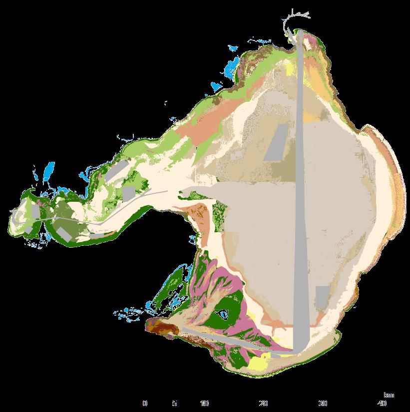
5% of coverage), these values were filled by spline
       interpolation.

       Table 2. Environmental Predictors used in habitat model. For full
       details of predictors see Appendix Table 1.

          Environmental
                                             Description
            Predictor
                               Calculated using the differential
       Aspect                  weighted algorithm (Horn 1981) for
                               DEMs
                               DEM from lidar and multibeam data
       Bathymetry
                               at 2.5 m resolution
                               Fetch 200 km offshore,
                               approximated as the minimum
       Distance to Coast
                               distance from shore in one of the
                               eight directions.
                               CBiCS energy classification ordinal         Figure 3. Examples of environmental predictor layers for Port
       Energy                  layer based on tidal currents, swell        Phillip Bay. Created in: ESRI (2019). ArcGIS Desktop: Release
                               ground surge and observed biotopes          10.8. Redlands, CA: Environmental Systems Research Institute.
       Exposure                Wind power, fetch (km), and depth
                               Lidar Reflectance at 5 m grid
       Light Reflectance                                                   Machine learning method
                               resolution resampled to 2.5 m
                               Calculated using the DEM, as the            Random Forest is an ensemble model using
                               greatest absolute difference                bagging as the ensemble method and decision tree
       Relief
                               between the centre cell and the             as the individual model (Breiman 2001). Ensemble
                               surrounding cells                           models incorporates multiple models to make overall
                               Calculated using the DEM and a              predictions, thus incorporates the variance within
       Ruggedness              Terrain Ruggedness Index (TRI;              different models to give results that are less
                               Riley et al. 1999).                         sensitive and that are more robust (less bias and
                               Rugosity was indexed by the square          less variance). Random Forest uses a bagging
                               root of the sum of the residuals            approach where subsets of the data are used to
                               when slope and aspect (Horn 1981)           train each model in parallel (not sequential; Figure
       Rugosity
                               were used to fit a plane to a 3 x 3         4). Random Forest is not affected by correlated
                               neighbourhood region and provide            variables as per other modelling approaches as it
                               residuals above and below the plane         uses a random selection of variables to build trees.
                               Compiled by Edmunds & Flynn
                               (2018) from: Beasely (1966); Currie         Random Forest is considered an effective modelling
       Sediment &              & Parry (1999); Poore (1992); Poore         method for marine habitats and biodiversity with
       Substratum              et al. (1975); Poore & Rainer (1976);       application across the globe, with high performance
                               Wilson et al. (1998); Cohen et al.          achieved in comparison to other methods (Wei et al.
                               (2000); Holdgate et al. (2001).             2010; Pitcher et al. 2012; Peterson & Herkul 2017;
                               Calculated using the differential           McLaren et al. 2019). To map the multiple habitat
       Slope                   weighted algorithm of Horn (1981)           types for the Level 3 Habitat complex in Port Phillip
                               for digital elevation models (DEMs)         Bay, the Random Forest classification algorithm was
                                A modified topographic position            used. Analyses were implemented in the R
                               index (Weiss 2001). Three                   computing environment (R Core Team, 2021) using
       Topographic
                               topographic index scales were               package “randomForest” (Liaw & Wiener, 2002). A
       Position Index                                                      total of 8,325 ground-truth records were used within
                               calculated: TPI a (5 m), TPI b – (25
                               m), TPI c (100 m).                          the model (of the 9,683 records) that met the
                                                                           Random Forest modelling criteria (≥5 unique values
                                                                           for each biotope category; Breiman 2001).

Port Phillip Bay Habitat Map                                                                                                 3
Habitat Complex Modelling (CBiCS Level 3)
                                                        OFFICIAL
Thalassia, Zostera), which are found near the
                                                                  coastline, particularly around Corio Bay. Saltmarsh
                                                                  and reedbeds (ba2.5; Boon et al. 2011), and
                                                                  mangroves (ba2.6; Edmunds & Flynn 2018) were
                                                                  not modelled in this study due to their different
                                                                  environmental variables as well as their well
                                                                  described distribution, these data were therefore
                                                                  joined to the habitat map after the modelling
                                                                  process. Several features of the bay such as the
                                                                  shipping channel and dredging areas were sections
                                                                  that were extracted from the habitat modelling
                                                                  process due to the altered habitat composition in
                                                                  these areas. These areas are depicted in grey.
Figure 4. Random Forest Classification. Source: Martinez, E. et
al. (2018).

Parameter tuning
The Random Forest algorithm can be tuned
according to parameter settings. A grid search
approach was applied based on the out-of-bag
(OOB) estimate of error to optimize the random
forest parameters. Three parameter which are
considered to influence the model were tuned; 1)
The number of variables randomly sampled as
candidates at each split (mtry), 2) the number of
trees to grow (ntree), and the maximum number of
terminal nodes that trees in the forest can have
(maxnodes).
Validation
Random Forest has inbuilt cross-validation using
bootstrapping. By default, Random Forest picks up
two-thirds of the data for training and rest for testing.
Trees are also constructed from randomised
variable selection and is not prone to overfit unlike
other models.

Habitat Complex Map (CBiCS Level 3)
The resulting Level 3 Habitat Complex map is
presented in Figure 5. Here the model represents 19
different habitat complexes at Level 3. The most
dominant habitat types are sublittoral sand and
muddy sand (ba5.2) and sublittoral mud (ba5.3)
within the centre of the bay. However, a diversity of
habitats are observed with other prominent habitats
of sublittoral seaweed on sediment (ba5.7) which
supports various seaweed communities as well as
drift algae mats, and non-reef sediment epibenthos
(ba5.b) characterised by mixed sublittoral sediments
covered by epibenthic biota including scallop beds,
seapen beds, Pyura and ascidians. The entrance of
the Bay is uniquely characterised by moderate
energy infralittoral rock (ba3.2) as well as patches of
                                                                  Figure 5. Habitat map of Port Phillip Bay (Level 3 CBiCS).
sublittoral seagrass beds (ba5.8; genera
                                                                  Created in R (R Core Team, 2021) and mapped in ArcGIS (ESRI
Cymodocea, Halophila, Posidonia, Ruppia,
                                                                  2019). Coordinate system: WGS 1984 UTM Zone 55S.

4   Port Phillip Bay Habitat Map
    Habitat Complex Modelling (CBiCS Level 3)
Map accuracy and uncertainty                            mapping is required as well as those that depict
                                                               lower levels of CBiCS classification (i.e., level 4 and
       Random forest modelling produced an accuracy
                                                               5). However, the map also serves as a first indicator
       (Out-of-bag) of 91%. Bathymetry, substratum,
                                                               of the potential presence of vulnerable or rare
       sediment, and distance were the most important
                                                               habitats that may exist within the larger habitat
       predictors in the model (Appendix Figure 2). For full
                                                               complex, and marks areas where further detailed
       a full description of habitat classes and their
                                                               mapping could be undertaken. The current habitat
       prediction user and producer accuracy as well as
                                                               map presented here provides broad habitat
       error commission and omission please see the
                                                               complexes across the bay and provides greater
       Appendix Table 2. The resulting raster data were
                                                               knowledge of the diversity across the bay as whole.
       processed into polygon data using the ArcGIS
                                                               This work can support the management of large-
       Conversion and Cartography tool sets (ESRI 2019;
                                                               scale habitat complexes, their condition, and their
       Appendix Figure 3). Polygon data were aggregated
                                                               alignment with other broad scale processes across
       at 25 metres and do not represent the fine resolution
                                                               the bay.
       from the raster data (2.5m; available for download
       from CoastKit). The polygonised data were also
       assessed against previous mapping products across
       the bay, satellite imagery and marine navigation        Continuous Improvements
       charts, with small edits made for alignment.            Habitat models can be easily improved as more
                                                               ground-truth data are obtained. Similarly, the
       Limitations of the model include the reliance upon
                                                               incorporation of relevant environmental predictor
       past ground-truthed data, where habitat changes
                                                               data such as hydrodynamics and satellite imagery
       and shifts may have occurred. Habitat areas
                                                               can help improve model performance. Finer
       depicted in this model may also represent areas
                                                               resolutions models and habitat maps to CBiCS level
       which are suitable for particular habitats, however,
                                                               4 to 6, can be achieved with the availability of more
       they may not exist in that exact location. For
                                                               data. The habitat model (level 3) and resulting map
       example, seagrass is largely ephemeral in the Bay
                                                               provides an updated broad-scale habitat map across
       varies where its growth is influenced by
                                                               Port Phillip Bay and provide a baseline for future
       environmental conditions. Habitats represented at
                                                               data to build upon.
       CBiCS level 3 will also comprise a mosaic of
       biotopes and in some cases the represented habitat
       will not accurately define the integrated habitat
       complexes. Similarly, the model relies upon             References
       environmental variables to find a niche of suitable
                                                               Beasely, A.W. (1966). Port Phillip Survey 1957-1963. Bottom
       parameters that characterise the habitat complex
                                                               Sediments, Memoirs of the National Museum of Victoria
       within the Bay. Hence, inclusion of other
                                                               Melbourne, No. 27.
       environmental variables may improve the accuracy
       of the results and importantly environmental            Boon, P.I. et al. (2011). Mangroves and coastal saltmarsh of
       variables also contain some degree of uncertainty.      Victoria: distribution, condition, threats and management. Report
                                                               to DSE, Bendigo. 513 pp.

                                                               Breiman, L. (2001). Random forests. Machine learning, 45: 5-32.
       Habitat Map Applications                                Cohen, B.F., Currie, D.R. and McArthur, M.A. (2000). Epibenthic
       The habitat complex (Level 3 CBiCS) map supports        community structure in Port Phillip Bay, Victoria, Australia. Marine
       knowledge of the broad scale distributions and          and Freshwater Research, 51: 689-702.
       extent of marine habitats within Port Phillip Bay.      Currie, D.R. and Parry, G.D., (1999). Changes to benthic
       Importantly, these habitats encompass a range of        communities over 20 years in Port Phillip Bay, Victoria, Australia.
       other species, for example sublittoral seagrass beds    Marine Pollution Bulletin, 38(1), pp.36-43.
       (ba5.8) may contains a diversity of seagrass species
       including genera Cymodocea, Halophila, Posidonia,       Edmunds, M. and Flynn, A. (2015). A Victorian Marine Biotope
       Ruppia, Thalassia, Zostera, which are not depicted      Classification Scheme. Australian Marine Ecology Report No.
       individually in the model. Some of these species        545. Melbourne.
       may be more vulnerable than others, and some may        Edmunds, M. and Flynn, A. (2018). CBiCS Classification of
       or may not be present within the habitat complex        Victorian Biotopes. Report to Department of Environment, Land,
       that is mapped. The map should be used at broad         Water and Planning. Australian Marine Ecology Report No. 560,
       scales of >25 m, and where detailed work of habitat     Melbourne. 176 pp.
       types is needed, for example to examine the
       potential impacts of developments, finer resolution

Port Phillip Bay Habitat Map                                                                                         5
Habitat Complex Modelling (CBiCS Level 3)
                                               OFFICIAL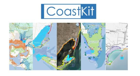
Edmunds, M., Flynn, A. and Ferns, L. (2021). Combined Biotope          Wilson, R.S., Heislers, S. and Poore, G.C. (1998). Changes in
Classification Scheme (CBiCS). A New Marine Ecological                 benthic communities of Port Phillip Bay, Australia, between 1969
Classification Scheme to Meet New Challenges. The State of             and 1995. Marine and Freshwater Research, 49: 847-861.
Victoria Department of Environment, Land, Water and Planning
                                                                       Weiss, A.D. (2001). Topographic Position and Landforms
2021.
                                                                       Analysis. Poster Presentation, ESRI User Conference, San
ESRI (2019). ArcGIS Desktop: Release 10.8. Redlands, CA:               Diego, July 2001. The Nature Conservancy.
Environmental Systems Research Institute.

Holdgate, G.R., Geurin, B., Wallace, M.W. and Gallagher, S.J.,
(2001). Marine geology of Port Phillip, Victoria. Australian Journal
of Earth Sciences, 48(3), 439-455.

Horn, B.K.P. (1981). Hill shading and the reflectance map:
Proceedings of the IEEE, 69: 14-47.

Liaw, A., and Wiener, M. (2002). Classification & regression by
randomForest. R News, 2: 18–22.

Martinez, E. et al. (2018), Evading deep neural network and
random forest classifiers by generating adversarial samples.
International Symposium on Foundations and Practice of
Security, 143-155.

McLaren, K., McIntyre, K. and Prospere, K. (2019). Using the
random forest algorithm to integrate hydroacoustic data with
satellite images to improve the mapping of shallow nearshore
benthic features in a marine protected area in Jamaica.
GIScience & Remote Sensing, 56(7), pp.1065-1092.

Peterson, A. and Herkül, K. (2019). Mapping benthic biodiversity
using georeferenced environmental data and predictive modeling.
Marine Biodiversity, 49: 131-146.

Poore, G.C. (1992). Soft-bottom macrobenthos of Port Phillip Bay:
a literature review. Technical Report No. 2, CSIRO.

Poore, G.C.B., Rainer, S.F., Spies, R.B. and Ward, E. (1975). The
zoobenthos program in Port Phillip Bay, 1969-73. Fisheries and
Wildlife Paper, Victoria. 1975; 7:1-78.

Poore, G.C. and Rainer, S., (1979). A three-year study of benthos
of muddy environments in Port Phillip Bay, Victoria. Estuarine and
Coastal Marine Science, 9: 477-497.

R Core Team (2021). R: A language and environment for
statistical computing. R Foundation for Statistical Computing.
http://www.R-project.org/

Riley, S.J., DeGloria, S.D. and Elliot, R. (1999). A terrain
ruggedness index that quantifies topographic heterogeneity,
Intermountain Journal of Sciences, 5:1-4.

Pitcher, C.R, Lawton, P., Ellis, N., Smith, S.J., Incze, L.S., Wei,
C.L., Greenlaw, M.E., Wolff, N.H., Sameoto, J.A. and Snelgrove,
P.V. (2012). Exploring the role of environmental variables in
shaping patterns of seabed biodiversity composition in regional‐
scale ecosystems. Journal of Applied Ecology, 49: 670-679.

Wei, C.L., Rowe, G.T., Escobar-Briones, E., Boetius, A.,
Soltwedel, T., Caley, M.J., Soliman, Y., Huettmann, F., Qu, F.,
Yu, Z. and Pitcher, C.R. (2010). Global patterns and predictions of
seafloor biomass using random forests. PloS one, 5: p.e15323.

6    Port Phillip Bay Habitat Map
     Habitat Complex Modelling (CBiCS Level 3)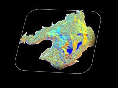
Appendix

       Table 1. Environmental predictors

         Predictors                 Description

         Bathymetry,                The data provided by DELWP included tiles of mixed lidar and multibeam data from 0.5 to 5 m grid resolution, (universal transverse Mercator projection, WGS84) and a state-
         Digital Elevation          wide combined product that included other hydrographic data at 10 m grid resolution (conical Lambertian projection - Vic Grid). The provided tiles were 10 x 10 km, and the
         Model (DEM)                tiling were set as a standard for state-wide raster mapping of marine habitats and biota. All provided data had a vertical datum of mean sea level (MSL). Lidar data for
                                    Gippsland Lakes was provided by DELWP separately and inserted into the DEM.

                                    The state-wide 10 m resolution grid was converted to Universal Transverse Mercator projection and tiled into 10 x 10 km tiles for zones 54 and 55 in Victoria. All data were
                                    then either up-scaled or down-scaled to a 2.5 m grid resolution in 10 x 10 km tiles. This resolution was chosen as being fine enough to map key marine habitats, particularly in
                                    the littoral zone, and be practical for data retrieval and computational analyses at a state-wide level. Data were down-scaled using bilinear interpolation and up-scaled using
                                    bicubic interpolation, with modelling and sharpening using a dual-tree discrete wavelet transform. A standard set of DEM tiles were then constructed by first constructing a set
                                    of blank tiles for the State, adding the down-scaled (high resolution) data and then filling the missing cells with the upscaled data. The Gippsland Lakes data were then
                                    inserted.

                                    The DEM was then converted from a vertical datum of mean sea level (MSL) to lowest astronomical tide (LAT) using spatial interpolations from the Australian Coastal Vertical
                                    Datum Tool. The interpolation points were derived from the spatial position of break points in the corrections from the tool. The standard tiles are divided into UTM Zone 54 and
                                    Zone 55 and saved as 4k x 4k byte arrays (.bin) with separate header (.hdr) and projection (.prj) files suitable for direct import to any GIS software. The position of the top left
                                    corner of the tile is indicated in the file name, enabling scripted and automatic data retrieval and handling.

         Lidar Reflectance          Lidar Reflectance was collected at 5 m grid resolution but was upscaled to 2.5 m resolution into tiles matching the DEM. The upscaling method was the same as for the
                                    bathymetry. The lidar reflectance data was not radiometrically corrected for depth and this should be considered for most habitat mapping purposes that cross ecological depth
                                    zones.

         Slope and Aspect           Fine-scale slope and aspect were calculated using the differential weighted algorithm of Horn (1981) for digital elevation models (DEMs). The algorithm was applied to a 3 x 3
                                    grid of cell size 2.5 m.

         Rugosity                   Rugosity was derived to provide a roughness measure relatively independent of slope, as opposed to most other texture indicators. In this case, the Horn slope and aspect
                                    was used to fit a plane to the 3 x 3 neighbourhood region and provide residuals above and below the plane. Rugosity was indexed by the square root of the sum of the
                                    residuals.

         Ruggedness and             Fine scale relief and ruggedness was calculated from the DEM using a 3 x 3 m grid of cells. Although the horizontal scale of the indices could be determined by a step size
         Relief                     between the cells, the calculation only used direct neighbours (matching slope, aspect and rugosity). For each centre cell, the elevation at the eight surrounding cells was
                                    extracted. Relief was calculated as the greatest absolute difference between the centre cell and the surrounding cells. Ruggedness was indicated using Riley et al. (1999)
                                    Terrain Ruggedness Index (TRI). This was calculated as the average of the squared elevation differences between the centre cell and the eight surrounding cells.

Port Phillip Bay Habitat Map                                                                                                     1
Habitat Complex Modelling (CBiCS Level 3)             OFFICIAL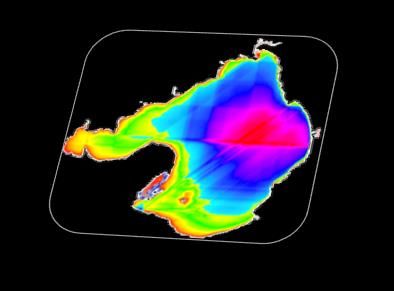
Topographic                A modified topographic position index (Weiss 2001) was used so the index could be calculated and compared at different scales. In this case the calculations were derived
                               from a circle of a selected number of points at a selected distance from a centre cell.
    Position Index
                               Data from a selected distance was used rather than the more traditional method of integrating data from the whole area within the circle, or from the area within an annulus, so
                               that different scaled data are not confounded by
                               the inclusion of data close to the centre cell. The circular data was extracted according to the estimated elevation of a point from each selected direction and radius from the
                               centre cell. This was estimated using bilinear interpolation from the four DEM cells surrounding the radius point of interest. Each index was calculated using 32 radials from the
                               centre cell.

                               Three topographic index scales were calculated:
                               TPI a - fine = 5 m (2 cell radius)
                               TPI b - medium = 25 m (10 cell radius)
                               TPI c - coarse = 100 m (40 cell radius)

    Distance from              Distance from shore, Fetch and Exposure was calculated using the DEM downscaled to 10 m grid scale then upscaled back to the standard tiles and scales. The downscaling
    Shore, Fetch and           was done to enable practical integral calculations over larger areas of the coast. All calculations were clamped at 60 km from the coast.
    Exposure                   A fetch index was calculated for each DEM cell as the sum of all distance steps to shore, in 8-point compass rose directions, out to the 60 m arbitrary limit. The fetch was
                               modified in shallow water < 5 m by a ramp function to account for wave breaking and sheltering by shoaling waters.

                               Distance from shore was approximated as the minimum distance from shore in one of the eight directions.

                               A relative exposure index was derived by integrating wind power with the fetch for each of the eight directions. The calculation used wind roses provided by the Bureau of
                               Meteorology for the locations of Mt Gambier, Cape Nelson, Warrnambool, Cape Otway, Lorne, Aireys Inlet, Queenscliff, Avalon, Melbourne, Cape Schanck, Wilsons
                               Promontory, Lakes Entrance, Point Hicks and Gabo Island. The wind speeds were converted to an approximation of power using the cube of speed in metres per second,
                               weighted by the frequency of occurrence for each wind speed category and totalled for each direction. The exposure index was calculated for each cell as a product of the
                               wind power and the fetch, summed over each of the eight directions. A gaussian smoothing function was then used to remove some of the quantisation imposed by the small
                               number of directions assessed.

    Sediment &                 Compiled by Edmunds & Flynn (2018) from: Beasely (1966); Currie & Parry (1999); Poore (1992); Poore et al. (1975); Poore & Rainer (1976); Wilson et al. (1998); Cohen et al.
    Substratum                 (2000); Holdgate et al. (2001).

    Energy                     CBiCS energy classification ordinal layer based on tidal currents, swell ground surge and observed biotopes. The open coast is classified as high energy and embayment’s are
                               low energy, with moderate energy zones connecting the high and low zones. In Victoria, there are not that many moderate energy zones, for Port Phillip Bay these include Port
                               Phillip Heads (inside Rip Bank to northern edge of Great Sands and eastward to Rosebud).

2     Port Phillip Bay Habitat Map
      Habitat Complex Modelling (CBiCS Level 3)
Table 2. The Random Forest habitat model accuracy, overall accuracy of 91%.
User Error
Accuracy Commission
ba11 ba12 ba13 ba22 ba23 ba26 ba31 ba32 ba33 ba42 ba51 ba52 ba53 ba54 ba56 ba57 ba58 ba5b ba5c ba5d % %
ba11 60 1 0 0 0 0 0 0 0 0 0 0 0 0 0 0 0 0 0 0 98.36 1.64
ba12 0 28 2 0 0 0 0 2 0 0 0 0 0 0 0 0 0 0 0 0 87.50 12.50
ba13 0 0 249 1 0 0 0 0 2 0 0 0 0 0 1 0 6 0 0 0 96.14 3.86
ba22 0 0 2 67 0 0 0 0 1 0 0 0 0 0 0 0 25 0 0 0 70.53 29.47
ba23 0 0 0 0 10 0 0 0 0 0 0 0 0 0 0 0 24 0 0 0 29.41 70.59
ba26 0 0 2 2 0 3 0 0 0 0 0 0 0 0 0 0 2 0 0 0 33.33 66.67
ba31 0 0 1 0 0 0 342 30 0 1 0 2 0 0 0 0 0 0 0 0 90.96 9.04
ba32 0 0 0 0 0 0 43 655 0 0 0 0 0 0 0 0 9 0 1 0 92.51 7.49
ba33 0 0 8 1 0 0 0 0 282 0 0 8 0 0 1 8 20 3 0 0 85.20 14.80
ba42 0 0 0 0 0 0 1 2 0 2 0 0 0 1 0 0 0 0 0 0 33.33 66.67
ba51 0 0 0 0 0 0 0 0 1 0 8 2 1 0 0 2 0 3 0 0 47.06 52.94
ba52 0 0 0 0 0 0 1 1 11 0 0 1741 0 1 1 28 73 5 0 0 93.50 6.50
ba53 0 0 0 0 0 0 0 0 0 0 0 19 28 3 0 13 1 0 0 5 40.58 59.42
ba54 0 0 0 0 0 0 0 1 0 1 0 14 6 5 0 1 5 9 5 0 10.64 89.36
ba56 0 0 1 1 0 0 0 0 2 0 0 1 0 1 50 3 26 6 0 0 54.95 45.05
ba57 0 0 0 1 0 0 0 0 7 0 1 50 1 2 2 985 26 7 0 0 91.04 8.96
ba58 0 0 2 2 0 0 0 20 7 0 1 65 0 0 9 22 2738 2 1 0 95.43 4.57
ba5b 0 0 0 0 0 0 0 0 4 0 0 4 1 1 3 9 5 275 2 0 90.46 9.54
ba5c 0 0 0 0 0 0 0 0 0 0 0 7 0 1 1 2 3 2 33 0 67.35 32.65
ba5d 0 0 0 0 0 0 0 0 0 0 0 2 7 2 0 0 0 0 0 13 54.17 45.83
Producer
Accuracy
% 100.00 96.55 93.26 89.33 100.00 100.00 88.37 92.12 88.96 50.00 80.00 90.91 63.64 29.41 73.53 91.80 92.41 88.14 78.57 72.22
Error Overall Accuracy 91%
Omission
% 0.00 3.45 6.74 10.67 0.00 0.00 11.63 7.88 11.04 50.00 20.00 9.09 36.36 70.59 26.47 8.20 7.59 11.86 21.43 27.78
Port Phillip Bay Habitat Map 3
Habitat Complex Modelling (CBiCS Level 3) OFFICIAL3500
3000
2500
Frequency
2000
1500
1000
500
0
1969 1970 1996 1998 1999 2000 2001 2002 2003 2004 2005 2006 2007 2009 2010 2011 2012 2013 2014 2015 2019
Year
ba11 ba12 ba13 ba22 ba23 ba25 ba26 ba31 ba32 ba33 ba42
ba51 ba52 ba53 ba54 ba56 ba57 ba58 ba5b ba5c ba5d
Figure 1. Ground-truth records across Port Phillip Bay (biotope level 3 habitat level) sampled per year from 1969 to 2019.
4 Port Phillip Bay Habitat Map
Habitat Complex Modelling (CBiCS Level 3)Figure 2. Environmental predictor importance from the Random Forest model. Bathymetry, substratum, sediment and distance were the most important
predictors in the model.
Port Phillip Bay Habitat Map 5
Habitat Complex Modelling (CBiCS Level 3) OFFICIALFigure 3. Habitat map of Port Phillip Bay (Level 3 CBiCS). Created in R (R Core Team, 2021) and mapped in ArcGIS (ESRI 2019). Coordinate system:
WGS 1984 UTM Zone 55S; A) polygon data aggregated at 25 metres with minor edits made to align with previous mapping products across the bay,
satellite imagery and marine navigation charts B) fine resolution raster (2.5m; available for download from CoastKit) output from random forest
classification model.
6 Port Phillip Bay Habitat Map
Habitat Complex Modelling (CBiCS Level 3)You can also read