Privacy-Preserving Publication of Time-Series Data in Smart Grid - Hindawi.com
←
→
Page content transcription
If your browser does not render page correctly, please read the page content below
Hindawi
Security and Communication Networks
Volume 2021, Article ID 6643566, 21 pages
https://doi.org/10.1155/2021/6643566

Research Article
Privacy-Preserving Publication of Time-Series Data in Smart Grid

 Franklin Leukam Lako ,1,2 Paul Lajoie-Mazenc ,2 and Maryline Laurent 1

 1
 Department of Network and Telecommunication Services, Samovar Lab, Télécom SudParis, Institut Polytechnique de Paris,
 19 rue Marguerite Perey, Palaiseau 91120, France
 2
 EDF Lab Paris-Saclay, 7 Boulevard Gaspard Monge, Palaiseau 91120, France

 Correspondence should be addressed to Franklin Leukam Lako; franklin.leukam-lako@edf.fr

 Received 4 December 2020; Revised 18 February 2021; Accepted 2 March 2021; Published 26 March 2021

 Academic Editor: Chalee Vorakulpipat

 Copyright © 2021 Franklin Leukam Lako et al. This is an open access article distributed under the Creative Commons Attribution
 License, which permits unrestricted use, distribution, and reproduction in any medium, provided the original work is
 properly cited.

 The collection of fine-grained consumptions of users in the smart grid enables energy suppliers and grid operators to propose new
 services (e.g., consumption forecasts and demand-response protocols) allowing to improve the efficiency and reliability of the grid.
 These services require the knowledge of aggregate consumption of users. However, an aggregate can be vulnerable to rei-
 dentification attacks which allow revealing the users’ individual consumption. Revealing an aggregate data is a key privacy
 concern. This paper focuses on publishing an aggregate of time-series data such as fine-grained consumptions, without indirectly
 disclosing individual consumptions. We propose novel algorithms which guarantee differential privacy, based on the discrete
 Fourier transform and the discrete wavelet transform. Experimental results using real data from the Irish Commission for
 Regulation of Utilities (CRU) demonstrate that our algorithms achieve better utility than previously proposed algorithms.

1. Introduction particular, forecasting enables the supplier to predict future
 consumptions based on past aggregate data in order to
A smart city is a designation given to a city that incorporates improve the grid and retail operations and enhance energy
information and communication technologies to enhance trading [4], while demand-response (DR) aims to shift the
the quality and performance of urban services such as en- users’ consumption from peak to off-peak periods in order
ergy, transportation, and utilities in order to reduce resource to avoid consumption peaks in the smart city.
consumption, wastage, and overall costs. The overarching However, aggregates are vulnerable to reidentification
aim of a smart city is to enhance the quality of living for its attacks, such as set difference attacks [5] in which two ag-
citizens through smart technology [1–3]. gregates that differ by a single consumer allow learning this
 The smart grid is an important part of the smart city. individual consumption. Since the individual consumption
Indeed, the smart grid allows greater penetration of highly data collected by smart meters reflect the use of all electric
variable renewable energy sources such as solar and wind appliances by inhabitants in a household over time and
power in the smart city. enable to deduce the behaviors, activities, age, or preferences
 The smart grid modernizes the traditional electricity grid of the inhabitants [6–11], revealing an aggregate is a key
by establishing a communication infrastructure in parallel to privacy concern.
the energy delivery network. This infrastructure is used by Differential privacy (DP) [12] allows publishing an ag-
the grid operators and suppliers to remotely collect fine- gregate data while guaranteeing that an attacker does not
grained consumptions from household smart meters and to learn any individual inputs from the aggregate. However, the
provide new energy services such as consumption forecasts noise added by DP often leads to a loss of utility. Moreover,
or demand-response. These services are suitable for im- publishing time-series data such as users’ consumption,
proving the efficiency and reliability of the grid, saving which are correlated, by using DP, results in more noise
energy and, more generally, for optimizing energy usage. In added than publishing a single aggregate for the same
2 Security and Communication Networks

privacy guarantee. Thus, disclosing time-series data leads to Table 1: List of acronyms.
more loss of utility. Utility can be improved by increasing the
 Acronym Meaning
size of the aggregate. Eibl and Engel [13] showed that for
real-world smart metering, the aggregation group size must CFPA Clamping Fourier perturbation algorithm
 CWPA Clamping wavelet perturbation algorithm
be of the order of thousands of smart meters in order to have
 DFT Discrete Fourier transform
reasonable utility. This paper shows how to obtain good DP Differential privacy
utility with a group size smaller than 600. We obtain a mean DWT Discrete wavelet transform
relative error lower than 10% between the original data and FPA Fourier perturbation algorithm
the published one, which is considered practically suitable by MRE Mean relative estimation error
energy experts for consumption forecasts. WPA Wavelet perturbation algorithm
 The Laplace mechanism [14] is a popular mechanism to
enable DP, by adding independent and identically distrib- while supporting energy services such as demand-response,
uted (IID) Laplace noise to each component of the time- smart metering, billing, or forecasting.
series. However, adding IID noise for correlated time-series In this paper, we investigate tools enabling forecasting
is not appropriate. In fact, an adversary can use refinement and demand-response. In particular, we are interested in
methods, such as filtering, to sanitize the IID noise and publishing an aggregate of individual consumptions, while
improve the probability of disclosing individual data preserving privacy.
[15, 16]. Differential privacy (DP), introduced by Dwork in 2006,
 This paper focuses on disclosing an aggregate of users’ guarantees that the publication of an aggregate does not
consumption data without learning individual data and indirectly reveal the individual data [12]. Moreover, DP
proposes methods with improved utility. We summarize our guarantees that two aggregates that differ by a single con-
contributions as follows: sumer are almost indistinguishable. DP has evolved over-
 time [31] and was adopted by organizations such as the US
 (i) We revisit the Fourier perturbation algorithm
 Census Bureau [32], Google [33], Apple [34], and Microsoft
 (FPA) [17] in order to correct some mistakes leading
 [35]. The Laplace mechanism [14] is a popular mechanism
 to poor users’ privacy protection. We show that, in
 that allows guaranteeing DP by adding a noise drawn from
 order to√��ensure
 � the desired budget of privacy ϵ, a
 the Laplace distribution L(·) to the aggregate.
 factor 2T must be added to the noise, where T is
 The Laplace mechanism takes as input two parameters:
 the size of the time-series. However, this reduces the
 the privacy budget ϵ and the sensitivity of the function to
 utility of FPA.
 publish (in our case, the sum of users’ consumption).
 (ii) We propose the “clamping Fourier perturbation Smaller values of ϵ lead to a better protection, but add a
 algorithm (CFPA)” using the clamping mechanism bigger noise to the aggregate.
 proposed in [18], for reducing the sensitivity, and Utility can be improved by increasing the size of the
 thus the noise introduced in FPA. This new algo- aggregate in order that the effect of noise is small enough
 rithm is an improvement of the Fourier perturba- that the result can be utilized. Eibl and Engel [13] showed
 tion algorithm (FPA). Experimental results show a that for real-world smart metering, the aggregation group
 utility improvement by a factor more than 6. size must be of the order of thousand smart meters in order
 (iii) We also propose the “clamping wavelet perturba- to have reasonable utility. This paper shows how to obtain
 tion algorithm” (CWPA), a similar adaptation of good utility with a group size smaller than a thousand.
 wavelet perturbation algorithm (WPA) [19], with a DP is typically applied to static data, i.e., to a single
 utility improvement by a factor 2. query. In this paper, we consider time-series consumption,
 (iv) We compare FPA, CFPA, WPA, and CWPA by which is equivalent to multiple queries on correlated data.
 analyzing their relative errors on a real dataset, and Applying the Laplace mechanism independently to each data
 we explain why CFPA obtains the best utility. point of the time-series is not appropriate. Indeed, an ad-
 versary can use refinement methods, such as filtering, to
 The remainder of this paper is structured as follows. sanitize the Laplace noise and improve the probability
Section 2 provides an overview of the literature, while disclosing individual data [15, 16]. Thus, the data points of
Section 3 presents preliminaries. Section 4 correctly com- the time-series are correlated. The composition theorem [14]
putes the sensitivity of DFT in order to make FPA ϵ-dif- states that the privacy budget ϵ of T correlated queries adds
ferentially private. Section 5 details our privacy-preserving up, i.e., setting the privacy budget for a single query to
publication techniques using clamping mechanism, DFT, εq � 0.5, the privacy budget of T � 48 single queries (cor-
and DWT. Section 6 reports our experimental results. responding to a day profile with a time interval of 30 min) is
Section 7 concludes the paper. ε � 0.5 × 48 � 24. In order to guarantee a global privacy
 Table 1 lists the acronyms used in this paper. budget of ε, one solution is to set the privacy budget of each
 query to ε/T. Of course, this leads to more noise in the
2. Related Work aggregate and a loss of utility.
 One method to guarantee DP for correlated time-series
Demand-response protocols [20–23], and secure aggrega- data publishing consists in transforming the original cor-
tion protocols [24–30] aim to protect the privacy of users related time-series into another representation while
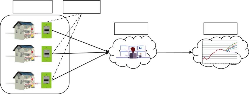
Security and Communication Networks 3

 j
maintaining its major characteristics before adding the consumptions collected by SM j, where xt is the con-
Laplace noise. Rastogi and Nath [17] proposed the Fourier sumption at time slot t (t � 1, . . . , T) collected by SM j
perturbation algorithm (FPA) that combines discrete (j � 1, . . . , N), with T being the time period considered.
Fourier transform (DFT) with DP to support time-series of Each time-series consumption Xj is sent to an aggregator
count queries while not disclosing any individual data and who computes the following aggregate:
ensuring good utility. We note that the sensitivity of count N N N
queries is 1, and the global sensitivity is T for a time-series of j j
 ⎝ x , x , . . . , x ⎞
 S � S1 , . . . , ST � ⎛ ⎠ j
 1 2 T . (1)
length T. Ács et al. [36] proposed an optimization of the FPA j�1 j�1 j�1
allowing to release histograms, where the global sensitivity is
1. They show through experimental evaluation that their To reveal S to a forecaster without indirectly disclosing
scheme improves the utility of the initial FPA by a factor 10. individual consumptions Xj (j � 1, . . . , N), the aggregator
Lyu et al. [19] applied FPA to time-series consumptions and can use differential privacy (DP).
proposed wavelet perturbation algorithm (WPA) by
replacing DFT by discrete wavelet transform (DWT). The
authors show through experimental results that WPA en- 3.2. Differential Privacy. Differential privacy is a framework
sures better utility than FPA. introduced by Dwork allowing quantifying the privacy
 We apply these approaches to time-series of con- guarantees of a request on a database [38]. This request can
sumption data and refine them by reducing the sensitivity of be the publication of a database, or a more precise one, such
the queries in order to reduce the relative error of the final as “what is the sum of energy consumptions of users in this
result. database?”.
 A request on databases is said to be differentially private
 if this request makes two similar databases indistinguishable
3. Preliminaries from looking only at the output of the request. Differential
 privacy relies on a parameter, noted ε, called the privacy
3.1. System and Threat Model. The entities involved in this
 budget. The formal definition of a differentially private al-
paper are as follows:
 gorithm is given as follows.
 (i) Trustworthy homes, which smart meter (SM) en-
 ables to collect their true individual time-series Definition 1 (ε−differentially private). A request
 consumption. A: D ⟶ S is ε−differentially private if and only if for all
 (ii) A honest aggregator, which collects users’ indi- databases D1 , D2 ∈ D differing by at most one record, and for
 vidual consumption, and which publishes an ag- all subsets O ⊂ S,
 gregate time-series consumption of users to a
 Pr A D1 ∈ O ≤ exp(ε)Pr A D2 ∈ O . (2)
 forecaster in a privacy-preserving way for the
 forecaster not to be able to deduce any individual
 consumption of users. This definition can be applied not only to requests on
 (iii) A forecaster, which predicts future consumptions databases but also to any function, by considering the do-
 based on the aggregate consumption received in main of the function as a database format.
 order to improve the grid and retail operations and Dwork also proposes the Laplace mechanism, which
 enhance energy trading. The forecaster is considered allows making any (vectors of ) real-valued function ε-dif-
 honest-but-curious as it provides appropriate ferentially private [38]. This mechanism relies on the notion
 forecasts, but it may attempt to infer the users’ of sensitivity of a function, which represents how a single
 individual consumption from the aggregate in order record of the database can influence the output of the
 to deduce the behaviors, activities, age, or prefer- function.
 ences of the inhabitants.
 Figure 1 depicts the system model. In a real scenario, the Definition 2 (sensitivity). Let f: D ⟶ Rd be a function;
aggregator can be an energy distributor, and the forecaster the sensitivity of f is
 �� �
can be a municipality that seeks to find out the total con- Δ1 (f) � max ��f D1 − f D2 ��� .
sumption of the inhabitants of the municipality. D1 ,D2 ∈D s.t. d(D1 ,D2 ) ≤ 1
 1 (3)
 Considering the case where the aggregator and the
forecaster belong to two entities of the same energy provider,
the publication of aggregate users’ consumption to fore- This sensitivity is also called L1 -sensitivity due to the
casters in a privacy-preserving way reduces the risk of L1 −norm used in its definition and is denoted by Δ1 (f).
disclosing users’ individual consumption. Moreover, this Similarly, the L2 -sensitivity used later and denoted by ε is
avoids the need for forecasters to ask for explicit consent computed using the L2 −norm (the L1 −norm and the L2
from customers in accordance with the GDPR [37] to norm of a vector S � (s1 , . , sT ) are
 . .����� � respectively equal to
process their personal data. ‖S‖1 � Tj�1 |sj | and ‖S‖2 � Tj�1 s2j ).
 Let N be the number of smart meters (SMs) in a district. The Laplace mechanism consists of adding a random
 j j j
Let Xj � (x1 , x2 , . . . , xT ) be the time-series of energy value to the original result of the query, where the random
4 Security and Communication Networks

 Smart meters
 Homes
 (SMs)

 Aggregator Forecaster

 ... ...

 Figure 1: System model.

value follows the Laplace distribution, where the parameter Moreover, the noisy version has inconsistent values such as
depends on the chosen ϵ and on the sensitivity of the negative consumptions.
function, as follows.
 Rastogi and Nath [17] introduce the Fourier perturba-
Theorem 1 (Laplacian mechanism). For all functions tion algorithm (FPA) and show that is an effective tool for
f: D ⟶ Rd , the algorithm A(D) � f(D) +(L1 (Δ1 reducing the noise introduced by the Laplace mechanism for
(f)/ε), . . . , Ld (Δ1 (f)/ε)) is ϵ−differentially private, where time-series. Section 3.3 presents the FPA. However, there are
L(·) is the distribution of Laplace and Δ1 (f) is the sensitivity some mistakes in this version relying on the estimation of
of f. the FPA sensitivity. These mistakes are presented in Section
 4, along with the corrected FPA.
 DP introduces noise in order to guarantee privacy. This Table 2 lists the symbols used in the rest of the paper.
noise can decrease the utility of the function. We quantify
this loss using mean relative estimation error (MRE), defined 3.3. Fourier Perturbation Algorithm. The Fourier perturba-
as follows. tion algorithm (FPA) presented in [17, 19, 36] takes as input
 a time-series S � (S1 , . . . , ST ) and an integer k ≪ T and
Definition 3 (mean relative estimation error). The mean returns the noisy time-series S � ( S1 , . . . , ST ), as shown in
relative estimation error (MRE) between two vectors a and b Algorithm 1.
of size T is 1/T · Tj�1 |aj − bj |/aj + 12 (we add 1 to the Rastogi and Nath [17] show that FPA is ε−differentially
denominator in order to avoid dividing by zero. This def- private. However, there are some mistakes in their proof of
inition is also used in [27]). Theorem 4.1 of [17] which justified that FPA is ε-differen-
 tially private. These mistakes rely on the estimation of the
 Consider the aggregate S � (S1 , . . . , ST ) defined in (1). FPA sensitivity and are presented in Section 4.
Let M be the maximum consumption in the domain. One
naive solution to publish S without revealing any individual 3.4. Wavelet Perturbation Algorithm. By replacing the DFT
consumption is to use the Laplace mechanism to add in- with the discrete Haar wavelet transform (DWT), Lyu et al.
dependent Laplace noise to each component of S and to [19] proposed the wavelet perturbation algorithm (WPA)
release the results: S � (S1 + L(M · T/ε), . . . , ST +
 and showed that WPA guarantees better utility than DFT.
L(M · T/ε)), where the sensitivity of the sum of time-series Algorithm 2 describes WPA.
consumption is M · T. However, this simple approach leads Figure 3 shows the same aggregated consumption presented
to excessive noise rendering the aggregate useless [13]. in Example 1 and its noisy version using WPA (Algorithm 2)
 with Haar wavelet, ε � 1 per day and k � 5. In Figure 3, the
Example 1. Figures 2(a) and 2(b), respectively, show the MRE is however higher than 10% (18%). In the noisy aggregate,
aggregated consumption of 250 homes from December 30th, the first peak of the morning is masked and the peak of the
2009, to January 5th, 2010, taken from the CER dataset [39], evening is truncated, as well as the trough of the night.
and its noisy version using the naively applied Laplace
mechanism, with ε � 1 per day. Figure 2(a) shows two Theorem 2. Wavelet perturbation algorithm (WPA) is
consumption peaks at 12 am and 6 pm which respectively ε-differentially private.
correspond to lunch and dinner time. We also observe that
in the night (from 12 pm to 6 am) the consumption de- Proof. DWT is orthonormal [40], i.e., W has the same L2
creases. Figure 2(b) shows that the noisy version is com- norm as S, that is, Δ2 (W) � Δ2 (S). Furthermore,
pletely different from the original aggregate (Figure 2(a)). In Δ2 (Wk ) ≤ Δ2 (S) (because T − k DWT coefficients √�of W are
 k
this example, the MRE between the aggregate consumption set to 0). With the inequality
 √� of norm,
 √���Δ 1 (W ) ≤ kΔ2 (Wk ).
 k
and the noisy version is 141%, which is not usable. Then, Δ1 (W ) ≤ kΔ2 (S) ≤ M · kT. Thus, the noise
Security and Communication Networks 5

 1000
 250
 750
 Consumption (kWh)

 Consumption (kWh)
 200 500
 250
 150 0
 –250
 100
 –500
 50 –750
 2009-12-30

 2009-12-31

 2010-01-01

 2010-01-02

 2010-01-03

 2010-01-04

 2010-01-05

 2009-12-30

 2009-12-31

 2010-01-01

 2010-01-02

 2010-01-03

 2010-01-04

 2010-01-05
 (a) (b)

Figure 2: Aggregated time-series consumption of 250 homes from December 30th, 2009, to January 5th, 2010, taken from the CER dataset
[39], and its noisy version using the naively applied Laplace mechanism, with ε � 1 per day. (a) Aggregated consumption. (b) Noisy version
using the naive solution.

 Table 2: List of symbols.
Notation Description
N Number of smart meters (SMs) in the district
M Maximum consumption in the dataset
T Time period during the collection of time-series consumption
 j
 j j j Time-series of energy consumptions collected by SM j, where xt is the consumption at time slot t (t � 1, . . . , T)
Xj � (x1 , x2 , . . . , xT )
 collected by SM j (j � 1, . . . , N)
 j
S � (S1 , . . . , ST ) Sum of users’ time-series consumptions to be published, where St � Nj�1 xt for t � 1, . . . , T
ε Budget of privacy
 S Noisy version of S
 Number of the first DFT or DWT coefficients conserved in the Fourier perturbation algorithm (FPA), wavelet
 k perturbation algorithm (WPA), clamping Fourier perturbation algorithm (CFPA), and clamping wavelet
 perturbation algorithm (CWPA)
 Δ1 L1 -sensitivity
Δ2 L2 -sensitivity

 Inputs: S � (S1 , . . . , ST ), k, the maximum consumption M of the domain, and the privacy budget ϵ.
 (1) Compute the discrete Fourier transform of S: F � DFT(S).
 (2) Keep only the first k coefficients of F, denoted by Fk .
 √���
 (3) Generate the noisy version of Fk , denoted by F k by adding a Laplace noise L(M Tk /ε) to each coefficient in Fk .
 k k
 (4) Pad F to a T-dimensional vector, denoted by PADT (F ) by appending T − k zeroes.
 (5) Apply the inverse DFT to PADT (F k ) to obtain a noisy version of S denoted by S.

 ALGORITHM 1: Fourier perbutation algorithm [17].

 Inputs: S � (S1 , . . . , ST ), k, the maximum consumption M of the domain, and the privacy budget: ε
 (1) Compute the DWT coefficients of S : W � DWT(S).
 (2) Keep only the first k coefficients of W, denoted by Wk . √���
 (3) Generate the noisy version of Wk , denoted by W k by adding a Laplace noise L(M Tk /ε) to each coefficient in Wk .
 k k
 (4) Pad W to a T-dimensional vector, denoted by PAD (W T ) by appending T − k zeroes.
 (5) Apply the inverse DWT to PADT (W k ) to obtain a noisy version of S denoted by S.

 ALGORITHM 2: Wavelet perbutation algorithm [19].
6 Security and Communication Networks

 300

 250

 Consumption (kWh)
 200

 150

 100

 50

 2009-12-30

 2009-12-31

 2010-01-01

 2010-01-02

 2010-01-03

 2010-01-04

 2010-01-05
 Aggregated consumption
 Noisy version (WPA), MRE = 18.367%
Figure 3: Aggregated consumption of 250 homes from 30th December 2009 to 5th January 2010 of dataset from CER [39] and its noisy
version using WPA (Algorithm 2), with Haar wavelet, ε � 1 per day and k � 5.

introduced in Step 3 is justified and WPA guarantees In [17, 19, 36], the authors use the latter version of DFT,
ε−differential privacy. □ which is not normalized. However, the sensitivity computation
 relies on the equality
 √�� ‖DFT(S)‖2 � ‖S‖2 , while it should be
 ‖DFT(S)‖
 √�� 2 � T · ‖S‖2 . Thus, the correct total privacy budget
4. Correctly Estimating the Sensitivity of FPA is T · ε instead of ε. This is the first mistake in this approach
In [17], authors show that FPA, as described in Section 3, and can be resolved by using the normalized DFT.
guarantees ε−differential privacy. Another error lies in the fact that the Laplacian mech-
 √��� The authors estimated√the
 ��
sensitivity of DFT to be M Tk, while it should be MT 2k, anism is only applied to the real part of the Fourier coef-
with T being the size of the time-series and M being the ficients, which are complex numbers. This mistake can be
maximum consumption in the domain. Thus, for a given resolved by applying the Laplace mechanism to both real and
privacy budget ε, the utility of FPA is worse than presented imaginary parts of the Fourier coefficients.
in [17]. The following section computes the sensitivity of the
 This section correctly computes the sensitivity of DFT, DFT, and thus of FPA, and takes into account those two
which allows to make render FPA ε−differential private. errors.
Before that we recall the definition of DFT.
 4.2. Sensitivity of the DFT. Let DFTk be the function which
 takes a time-series S � (S1 , . . . , ST ) as input and returns the
4.1. Discrete Fourier Transform (DFT). Let S � (S1 , . . . , ST ) first k DFT coefficients of S. This function can be seen as a
be a time-series. DFT takes S as input and returns a time- DFTk : RT ⟶ R2k , the function which returns the real and
series of T complex numbers F � (F1 , . . . , FT ) such that imaginary parts of the first k Fourier coefficients. This
 1 T function is a real-valued function, we can thus use the
 Fk � √�� Sj e− 2πi(j− 1)(k− 1)/T for k � 1, . . . , T, (4) Laplace mechanism on it. First, we need to compute the
 T j�1
 L1 -sensitivity of DFTk .
where i2 � −1. The inverse of the DFT is computed as
follows: Lemma 1. Let DFT k be defined as follows:
 k
 1 T DFTk : RT ⟶ R2
 Sk � √�� Fj e− 2πi(j− 1)(k− 1)/T , for k � 1, . . . , T. (5) (6)
 T j�1 S ⟼ DFTk (S) � a1 , b1 , . . . , ak , bk .
 This version of the DFT is normalized, that is,
‖DFT(S)‖2 � ‖S‖2 . √�� We denote cj � aj + ibj the j-th coefficient of DFT(S),
 DFTcan be defined in other ways, for instance, the 1/ T, with i2 � −1 and j � 1, . . . , k. aj and bj respectively repre-
present in both the DFT and the inverse definitions above, sent the real and imaginary parts of cj . √����
can be replaced by a factor 1 in the DFT and 1/T in the The L1 -sensitivity of DFTk , ‖DFTk (S)‖1 , is √ M��· 2Tk
inverse DFT. In that case, the DFT is not normalized. when the DFT is normalized (respectively, MT · 2k when
Security and Communication Networks 7

the DFT is not normalized), with M as the maximum value Proof. Let DFTk be defined as in Lemma 1.
in the dataset.

 �� �
 ��DFTk (S)��� � ���� a , b , . . . , a , b ����
 � �1 1 1 k k 1

 k � �� √� k �� ��
 �
 � ��� aj , bj ��� ≤ 2 ��� aj , bj ��� (Minkowski inequality))
 1 2
 j�1 j�1

 √� k
 ≤ 2 cj
 j�1
 √��� �� (7)
 ≤ 2�� c1 , . . . , ck ��1
 √�√��� ��
 ≤ 2 k�� c1 , . . . , ck ��2(Minkowski inequality)
 √���� ��
 ≤ 2k�� s1 , . . . , sT ��2 as T Fourier coefficients have the same L2 norm as S .
 Then,
 √�� √����
 Δ1 DFTk ≤ 2kΔ2 (S) � M 2Tk.

 □
 This result is true when the DFT is normalized (2) as in while they should be added to the real and imaginary
our case. In
 √��[17, 19, 36], the L2 norm of Fourier coefficients parts of the DFT coefficients as in the corrected FPA
equals to T times the L2 norm of S (Parvesal’s theorem). (Algorithm 3). Thus, k imaginary coefficients are not
This result is valid when the normalized DFT (2) is used as in noised in Algorithm 1.
our case. When the DFT is not normalized, as is the case in
 Figure 4 shows the same aggregated consumption pre-
[17, 19, 36], the sensitivity
 √�� of the first
 √���� k DFT √��coefficients
 k sented in Example 1 and its noisy version using the corrected
should
 √���be Δ1 (DFT ) � T × M 2Tk � MT 2k instead of FPA (Algorithm 3) with ε � 1 per day and k � 5. Figure 4
(M Tk). Thus, using the normalized DFT, the function
 shows that the corrected FPA obtains a large MRE (84%),
then becomes
 making it useless. The noisy aggregate has negative con-
 k
 sumptions and does not contain the peaks present in the
 DFTk : RT ⟶ R2
 original aggregate.
 � a , b , . . . , a , b + y , y , . . . , y , y ,
 S ⟼ DFT(S) 1 1 k k 1,1 1,2 k,1 k,2 For the sake of simplicity, in the following sections, we
 (8) use FPA to talk about the corrected version.
 √����
 which is ε−DP, with yj,ℓ � L(M 2Tk /ε), for all 5. Clamping Transform
 j � 1, . . . , k and ℓ � 1, 2. Perturbation Algorithm
 For simplicity,
 √���� in the following, we write
 + L(M
c√j ���� 2Tk√/ε)
 ���� instead of (aj , bj ) + (L(M The intuition behind our approach, “Clamping transform
 2Tk /ε), L(M 2Tk √ /ε)),
 ����meaning that two independent perturbation algorithm,” lies in the perturbation error,
 Laplace noises L(M 2Tk /ε) are added to the real and caused by the Laplace mechanism, which depends on the
 imaginary parts of cj . sensitivity of the sum of consumptions. As such, by reducing
 Algorithm 3 shows the Fourier perturbation algorithm the sensitivity, we expect to reduce the perturbation error.
(FPA) revisited. To estimate the sensitivity of consumptions, we split our
 database of N users into two almost equal parts: D1 cor-
 responding to the consumptions of the first half of users (a
4.3. Differences between the Initial, yet Incorrect, FPA, and the training dataset) and D2 containing the second half of users’
Corrected FPA. For a budget of privacy ε, the differences consumptions (a validation dataset). Using D1 , we compute
between the initial incorrect FPA and the corrected one can the distribution of users’ consumptions in the frequency
be highlighted as follows: domain. We denote by M � (M1 , . . . , Mk ) the maximum
 magnitude (by ignoring outliers) of the k first coefficients.
 (1) The DFT used in the initial incorrect FPA [17] is not For example, using the Irish consumption database [39],
 normalized, while it √ is��
 normalized
 � in the corrected the distribution of the individual consumption of the first
 FPA. Thus, a factor 2T is missing in the Laplace half customers (from 1 to 1818) in the frequency domain is
 noise in Algorithm 1. given in Figure 5. In Figure 5, the maximum magnitudes
 (2) In the initial incorrect FPA [17], Laplace noises are (rounded) of the 5 first coefficients are
 only added to the real part of the DFT coefficients, M � (M1 , M2 , M3 , M4 , M5 ) � (9, 4, 3, 2, 2).
8 Security and Communication Networks

 Inputs: S � (S1 , . . . , ST ), k, the maximum consumption M of the domain, and the privacy budget ε.
 (1) Compute the normalized DFT coefficients of S : F � DFT(S).
 (2) Keep only the first k coefficients of F, denoted by Fk . √����
 (3) Generate the noisy version of Fk , denoted by F k by adding a Laplace noise L(M 2Tk /ε) to each coefficient in Fk .
 (4) Pad F k to a T-dimensional vector, denoted by PADT (F k ) by appending T − k zeroes.
 T k
 (5) Apply the inverse DFT to PAD (F ) to obtain a noisy version of S denoted by S.

 ALGORITHM 3: Fourier perturbation algorithm (FPA) revisited.

 domain of the transform and keep the first k coef-
 j j
 300 ficients denoted by Cj � (C1 , . . . , Ck ).
 j
 (2) If the modulus of coefficient Cℓ is greater than Mℓ
Consumption (kWh)

 j j
 200 (1 ≤ ℓ ≤ k), replace Cℓ with Cℓ · Mℓ /|Cℓ | so that all
 coefficients have a modulus smaller than Mℓ and
 100 their phase, if the coefficient is complex, is
 unchanged.
 0
 (3) Compute the sum of coefficients
 j j
 –100 C � ( nj�1 C1 , . . . , nj�1 Ck ).
 (4) Add a noise following the distribution of Laplace
 L(·), depending on the sensitivity of the transform,
 2009-12-30

 2009-12-31

 2010-01-01

 2010-01-02

 2010-01-03

 2010-01-04

 2010-01-05

 to each coefficient Cℓ (1 ≤ ℓ ≤ k) of C. The result is
 denoted by C. We note that the Laplace noise is
 added to the real and imaginary parts of each co-
 Aggregated consumption efficient when the DFT is used.
 Noisy version (corrected FPA), MRE = 84.177% (5) Pad the vector C by n − k zeroes and compute the
Figure 4: Aggregated consumption of 250 homes from 30th inverse transform to obtain the noisy version of the
December 2009 to 5th January 2010 of dataset from CER [39] and consumption S.
its noisy version using the corrected FPA (Algorithm 3), with ε � 1 Section 5.1 presents an adaptation of this methodology
per day and k � 5.
 using the discrete Fourier transform.

 5.1. Clamping Fourier Perturbation Algorithm. This section
 70
 describes the clamping Fourier perturbation algorithm
 60 (CFPA) detailed in Algorithm 4. This algorithm allows an
 50 aggregator to compute and publish an aggregate guaran-
Magnitude

 teeing ε−differential privacy.
 40
 CFPA takes as inputs the individual time-series con-
 30 sumptions of n consumers, the maximum magnitudes of
 20 DFT coefficients of individual consumptions M (computed
 10
 over database D1 ), the number k of DFT coefficients to be
 considered, and the privacy budget ε, and it returns the noisy
 0 time-series sum of consumptions of n consumers.
 1 2 3 4 5 6 7 8 9 10 Step 1, called clamping, computes the first k DFT co-
 Coefficients (k) efficients of each individual time-series consumption. If the
 j
Figure 5: Distribution of users’ consumptions in the frequency magnitude of a coefficient Fℓ is greater than the maximum
domain using the discrete Fourier transform (DFT). magnitude Mℓ , then this coefficient is clamped and replaced
 j j j j
 by Fℓ · Mℓ /|Fℓ |, in which magnitude is |Fℓ | · Mℓ /|Fℓ | � Mℓ .
 Thus, for all individual consumptions Xj , the maximum
 The database D2 is used for testing our methodology. Let j j
 magnitude of the k first DFT coefficients Fj � (F1 , . . . , Fk ) is
X � (X1 , . . . , Xn ) with Xj � (xi1 , . . . , xiT ) for all j � 1, . . . , n
 M � (M1 , . . . , Mk ), i.e., the final values of the coefficients
be the users’ individual consumptions. To publish the sum of
 j j have the same phase as the initial values, but their magni-
consumptions S � (S1 , . . . , ST ) � ( nj�1 x1 , . . . , nj�1 xT ),
 tudes are bounded by (M1 , . . . , Mk ).
our methodology, which can be applied to either the Fourier
 After computing the first k DFT coefficients
transform or to wavelet transforms, is described as follows: j j
 Fj � (F1 , . . . , Fk ) of each individual time-series consump-
 (1) For all individual consumptions Xj (j � 1, . . . , n), tion of consumers (j � 1, . . . , n), Step 2 consists in com-
 j j
 compute the corresponding magnitude in the puting the sum (F1 , . . . , Fk ) � ( nj�1 F1 , . . . , nj�1 Fk ) of
Security and Communication Networks 9

 Inputs:
 (i) Consumptions: X � (X1 , . . . , Xn ) with Xi � (xi1 , . . . , xiT ) for all i � 1, . . . , n
 (ii) k
 (iii) The maximum magnitudes of k first DFT coefficients: M � (M1 , . . . , Mk ) ∈ Rk+
 (iv) Privacy budget: ε
 (1) Clamping: for each individual time-series consumption Xj ,
 j j
 (i) compute the k first DFT coefficients of Xj : Fj � (DFT(Xj )1 , . . . , DFT(Xj )k ) � (F1 , . . . , Fk )
 j j j j
 (ii) if |Fℓ | > Mℓ , then replace Fℓ with Fℓ · Mℓ /|Fℓ | for all ℓ � 1, . . . , k √�
 (2) Laplacian mechanism: compute the sum of noisy consumptions of each DWT coefficient: F ℓ � nj�1 Fjℓ + L(Mℓ 2 /ε/k) for all
 k
 ℓ � 1, . . . , k. We denote F � (F
 1, . . . , F
 k ). We note that the noise is added to the real and imaginary parts of the sum of
 coefficients.
 (3) Pad F k with T − k zeros; the result is denoted by PADT (F k)
 T k
 (4) Compute the inverse DFT of PAD (F ) to get the noisy sum of consumptions denoted by S � ( S1 , . . . , ST ) of the initial sum
 j j
 S � ( nj�1 x1 , . . . , nj�1 xT ).

 ALGORITHM 4: Clamping Fourier perturbation algorithm (CFPA).

 �� ��
these coefficients using the Laplacian mechanism. The result �� n n n n ��
 k � (F
 1, . . . , F
 k ). ��⎛
 ⎝ aj , bj ⎞ ⎠���
 ⎝ aj , b j ⎞
 ⎠ −⎛
is denoted by F Δ1 fℓ � max �
 Finally, the noisy sum of consumptions is equal to the aj , bj ��� j�1 j�1 ℓ ℓ
 j�2
 ℓ
 j�2
 ℓ ��
 �1
 ℓ ℓ

inverse of the noisy DFT coefficients padded with T − k �� ��
zeros. � max��� a1ℓ , b1ℓ ���
 1
 √��� ��
 ≤ max 2��� a1ℓ , b1ℓ ��� (Minkowski inequality)
 2
Theorem 3. Algorithm CFPA is ε-differentially private. �����������
 √� 2 2
 � max 2 a1ℓ + b1ℓ
Proof. To prove that Algorithm 4 is ε-differentially private, √�
we need to prove that the sensitivity of the sum of DFT � max 2 F1ℓ
 √�
coefficients of√�users’ individual √� consumptions √� F1 (resp. � Mℓ 2 .
F2 , . . . , Fk ) is 2 · M1 (resp. 2 · M2 , . . . , 2 · Mk ). This is
 (9)
done in Lemma 2. √�
 Then, as a Laplacian noise L(Mℓ 2 /ε/k) is added to □
each component Fℓ (ℓ � 1, . . . , k), the resulting F 1 (resp.

F2 , . . . , Fk ) is ε/k-differentially private. Finally, the com- Thus, Lemma 2 proves Theorem 3, and algorithm CFPA
position theorem [14] guarantees that any computation on guarantees ε-differential privacy.
the k components of (F 1, . . . , F
 k ) is ε-differentially private; For example, Figure 6 shows the same aggregated con-
thus, the inverse DFT of those coefficients is ε-DP. □ sumption presented in Example 1 and its noisy version using
 CFPA (Algorithm 4) with ε � 1 per day and k � 5. Figure 6
Lemma 2. Let Fj � (DFT(Xj )1 , . . . , DFT(Xj )k ) � shows that CFPA obtains a good utility with an MRE equal to
 j j
(F1 , . . . , Fk ) be the first k DFT coefficients of the individual 9.7%. This good utility of CFPA can be explained by the fact
consumption of consumer j (j � 1, . . . , n), obtained after the that Laplace noise added in CFPA depends on the amplitude
clamping mechanism. The sensitivity of the sum of each DFT of � coefficient, while in FPA, the same noise L(M ·
 each
 √���
 j
coefficient Fℓ (ℓ � √ 1,�. . . , k) of n consumers’ individual con- 2Tk /ε) is added to every DFT coefficients, where M is the
sumptions is Mℓ · 2. maximum consumption in the dataset.

 j j
Proof. Let Fj � (DFT(Xj )1 ,. .., DFT(Xj )k ) � (F1 , ... , Fk ). 5.2. Clamping Wavelet Perturbation Algorithm. The
 j
After the clamping, the magnitude of each DFTcoefficient Fℓ clamping wavelet perturbation algorithm (CWPA), as pre-
is smaller than Mℓ for ℓ � 1, ... , k, and the sensitivity of the sented in Algorithm 5, is obtained by replacing DFT with
function fℓ : Dn ⟶ C ≡ R2 defined by fℓ : (X1 , ... , Xn ) ⟼ DWT in Algorithm 4. The computation of DWT is based on
 j j j j j j
 nj�1 Fℓ ≡ ( nj�1 aℓ , nj�1 bℓ ), with Fℓ � aℓ + ibℓ being equal to multiresolution analysis which determines the number of
10 Security and Communication Networks

 300

 250

 Consumption (kWh)
 200

 150

 100

 50

 2009-12-30

 2009-12-31

 2010-01-01

 2010-01-02

 2010-01-03

 2010-01-04

 2010-01-05
 Aggregated consumption
 Noisy version (CFPA), MRE = 9.72%
Figure 6: Aggregated consumption of 250 homes from 30th December 2009 to 5th January 2010 of dataset from CER [39] and its noisy
version using CFPA (Algorithm 4), with ε � 1 per day and k � 5.

 j
approximation coefficients (scaling functions) and detail coefficient Wℓ is smaller than Mℓ for ℓ � 1, . . . , k, and the
coefficients (wavelet functions) [40]. DWT takes as input a sensitivity of the function wℓ : Dn ⟶ R defined by
 j
time-series of length a power of 2. If the input’s length is not wℓ : (X1 , . . . , Xn ) ⟼ nj�1 Wℓ is equal to
a power of 2, we can pad it with zeroes [41].
 n n
 Algorithm 5 takes as inputs the maximum magnitudes of j j
 Δ1 wℓ � max
 j Wℓ − Wℓ
the first k DWT coefficients which are obtained in the Wℓ j�1 j�2
training process on D1 , by computing the distribution of 1 (10)
DWT coefficients of individual consumptions. � max Wℓ
 We note that there are multiple DWTs, such as Haar, � Mℓ .
Daubechies, Symlets, and Coiflets. In this paper, we use Haar □
and Daubechies wavelets as shown in Section 6, because they
give a low reconstruction error, as will be discussed in For example, Figure 7 shows the same aggregated
Section 6.1. consumption presented in Example 1 and its noisy version
 using CWPA (Algorithm 5) with Haar wavelet, ε � 1 per day
Theorem 4. The clamping wavelet perturbation algorithm and k � 5. However, Figure 3 shows that the MRE of CWPA
(CWPA), Algorithm 5, is ε-differentially private. is still higher than 10%. We explain this result in Section 6.

Proof. The proof is similar to the one for Theorem 3. We 6. Experimental Results
need to prove that the sensitivity of the sum of DWT co-
efficients of users’ individual consumptions W1 (resp. This section compares FPA, CFPA, WPA, and CWPA and
W2 , . . . , Wk ) is M1 (resp. M2 , . . . , Mk ). This is done in explains through experimentations why CFPA achieves a better
Lemma 3. utility than other publication techniques. After presenting the
 Then, as a Laplacian noise L(Mℓ /ε/k) is added to each raw results, we explain them by decomposing the mean relative
component Wℓ (ℓ � 1, . . . , k), the resulting W 1 (resp. error into a perturbation error, caused by the clamping

W2 , . . . , Wk ) is ϵ/k-differentially private. Finally, the com- mechanism and the Laplace mechanism, and a reconstruction
position theorem [14] guarantees that any computation on error, due to ignoring T − k coefficients of the transform. The
the k components (W 1, . . . , W
 k ) is ϵ-differentially private; analysis of the error is thus conducted in the next two Sub-
thus, the inverse DWT of those coefficients is ϵ-DP. □ sections 6.1 and 6.2. Section 6.1 analyzes the reconstruction
 error, while Section 6.2 analyzes the perturbation one.
Lemma 3. Let Wj � (DWT(Xj )1 , . . . , DWT(Xj )k ) � Conditions: the experiments rely on data originating
 j j
(W1 , . . . , Wk ) be the first k DWT coefficients of the individual from the Irish Commission for Energy Regulation
consumption of consumer j (j � 1, . . . , n), obtained after the (CER) [39]. This dataset contains real time-series
clamping mechanism. The sensitivity of the sum of each DWT consumptions. The achieved results are valid for this
 j
coefficient Wℓ (ℓ � 1, . . . , k) of n consumers’ individual very specific case, for Irish consumptions with an Irish
consumptions is Mℓ . weather being never too hot or too cold. The results
 show that the approach is good, but will probably have
 j
Proof. Let Wj � (DWT(Xj )1 , . . . , DWT(Xj )k ) � (W1 , . . . , to be adapted for other datasets, i.e., by computing the
 j
Wk ). After the clamping, the magnitude of each DWT maximum magnitudes of the k first coefficients of the
Security and Communication Networks 11
Inputs:
j j
(i) Consumptions: X � (X1 , . . . , Xn ) with Xj � (x1 , . . . , xT ) for all j � 1, . . . , n
(ii) k
(iii) The maximum magnitudes of k first DWT coefficients: M � (M1 , . . . , Mk ) ∈ Rk+
(iv) Privacy budget: ε
(1) Clamping: for each individual time-series consumption Xj ,
j j
(i) compute the first k DWT coefficients of Xj : Wj � (DWT(Xj )1 , . . . , DWT(Xj )k ) � (W1 , . . . , Wk )
j j j i
(ii) if |Wℓ | > Mℓ , then replace Wℓ with Wℓ · Mℓ /|Wj | for ℓ � 1, . . . , k
(2) Laplacian Mechanism: compute the sum of noisy consumptions of each DWT coefficient: W ℓ � nj�1 Wjℓ + L(Mℓ /ε/k) for all
k
ℓ � 1, . . . , k. We denote W � (W
1, . . . , W
k)
(3) Pad W k with T − k zeroes; the result is denoted by PADT (W k)
T k
(4) Compute the inverse DWT of PAD (W ) to get the noisy sum of consumptions denoted by S � ( S1 , . . . , ST ) of the initial sum
j j
S � ( nj�1 x1 , . . . , nj�1 xT )
ALGORITHM 5: Clamping wavelet perturbation algorithm (CWPA).
300 represents the same wavelet as Daubechies with order 1,
noted db1), Daubechies with order 2, and Daubechies
250
with order 3, respectively, noted db2 and db3.
Consumption (kWh)
200 Raw results and analysis: Figures 8 and 9 show the
distribution of the mean relative estimation error
150 (MRE) according to the number of homes in the district
(N from 50 to 450) and k from 5 to 12 for the budget of
100 privacy ε � 1 and ε � 3, respectively. The boxes extend
from the lower to upper quartile values of the MRE,
50 with a line at the median and a triangle representing the
mean. The whiskers extend from the box to show the
2009-12-30
2009-12-31
2010-01-01
2010-01-02
2010-01-03
2010-01-04
2010-01-05
range of the MRE. In order to make consumption
forecasts, an MRE lower than 10% is required in
practice by experts in the energy sector. In this section,
Aggregated consumption an MRE of less than 10% is therefore considered useful.
Noisy version (CWPA), MRE = 16.31% In Figures 8 and 9, the first column corresponds to the
Figure 7: Aggregated consumption of 250 homes from 30th comparison between the FPA and the CFPA. The other
December 2009 to 5th January 2010 of dataset from CER [39] and columns correspond to the comparison between the WPA
its noisy version using CWPA (Algorithm 5), with Haar wavelet, and the CWPA using Haar wavelet with 2 approximation
ε � 1 per day and k � 5. coefficients, Daubechies 2 (db2) with 5 approximation co-
efficients, and Daubechies 3 (db3) with 10 approximation
considered transform over a subpart of the dataset. coefficients, respectively.
Consumption data from the CER were collected every Figures 8 and 9 show that CFPA has a better utility than
30 minutes from 2009 to 2010 with the participation of FPA. For example, for ε � 1 (Figure 8), when k � 5 and the
more than 5, 000 Irish homes and businesses. This number of homes N � 350, the MRE of CFPA is 12%, while
experiment only considers homes. We divided the the MRE of FPA is 75%. In that configuration, the MRE of
database in two parts: D1 , corresponding to the first half CFPA is 6.25 times lower than that of FPA. Similarly, the
of consumers (1 to 1818), and D2 , corresponding to the CWPA obtains a better utility than the WPA. For example,
second half (1819 to 3639). D1 is used to calibrate the for k � 5 and the number of homes N � 350, the MRE of
algorithms by computing the maximum magnitudes CWPA using Haar wavelet is 15%, while the MRE of the
M � (M1 , . . . , Mk ) of the first k coefficients in the WPA is 30%. In that configuration, the MRE of CWPA is 2
frequency domain, and D2 is used to test the publi- times lower than that of WPA.
cation techniques FPA, CFPA, WPA, and CWPA. Generally, the larger the size of the district N, the smaller
Notations: we note N as the number of homes or smart the MRE is. Similarly, the larger the budget of privacy ε, the
meters considered in the district to compute the time- smaller the MRE is; Figure 9 (ε � 3) shows a better utility
series of the sum of consumptions. For each day (48 time than Figure 8 (ε � 1). However, Figures 8 and 9 show that
slots), we compute the sum of consumptions of 50 WPA and CWPA using db3 are not useful for k � 5 because,
different districts of N random homes, and we execute as shown in Section 6.1, the reconstruction error is high
FPA, WPA, CFPA, and CWPA with privacy budget (between 70% and 80%).
ε ∈ {1; 3} for each day and k ∈ {5; 8; 12}. The discrete Figures 8 and 9 show that for larger k, the MRE of WPA
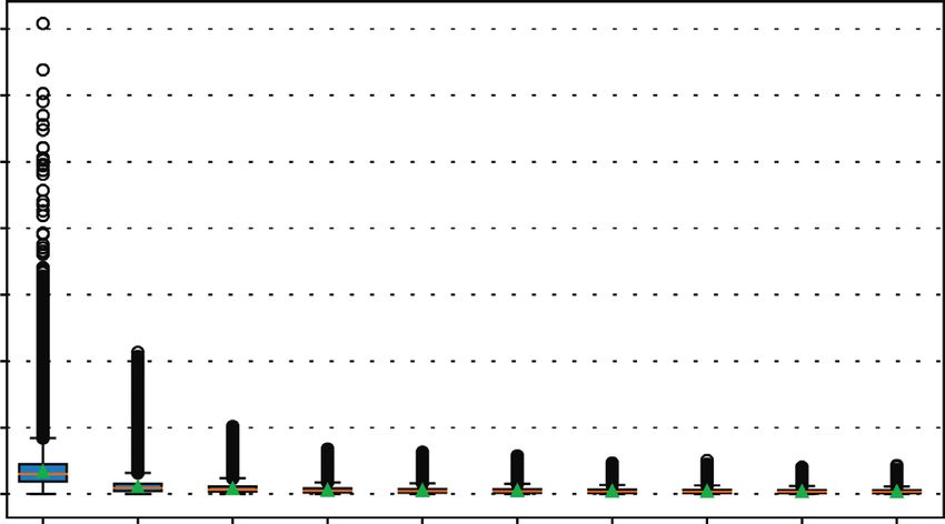
wavelet transforms used here are Haar transform (which and CWPA using db3 is smaller. Moreover, in Figure 9, for12 Security and Communication Networks Mean relative estimation error (MRE) Mean relative estimation error (MRE) Mean relative estimation error (MRE) k=5 k=5 k=5 101 101 101 100 100 100 10–1 10–1 10–1 50 150 250 350 450 550 50 150 250 350 450 550 50 150 250 350 450 550 FPA WPA-Haar 2cA WPA-db2 5cA CFPA CWPA-Haar 2cA CWPA-db2 5cA (a) (b) (c) Mean relative estimation error (MRE) Mean relative estimation error (MRE) Mean relative estimation error (MRE) k=5 k=8 k=8 101 101 101 100 101 101 10–1 10–1 10–1 50 150 250 350 450 550 50 150 250 350 450 550 50 150 250 350 450 550 WPA-db3 10 cA FPA WPA-Haar 2cA CWPA-db3 10 cA CFPA CWPA-Haar 2cA (d) (e) (f ) Mean relative estimation error (MRE) Mean relative estimation error (MRE) Mean relative estimation error (MRE) k=8 k=8 k = 12 1 1 1 10 10 10 101 101 101 10–1 10–1 10–1 50 150 250 350 450 550 50 150 250 350 450 550 50 150 250 350 450 550 WPA-db2 5cA WPA-db3 10 cA Number of smart meters (N) CWPA-db2 5cA CWPA-db3 10 cA FPA CFPA (g) (h) (i) Mean relative estimation error (MRE) Mean relative estimation error (MRE) Mean relative estimation error (MRE) k = 12 k = 12 k = 12 101 101 101 101 101 101 10–1 10–1 10–1 50 150 250 350 450 550 50 150 250 350 450 550 50 150 250 350 450 550 Number of smart meters (N) Number of smart meters (N) Number of smart meters (N) WPA-Haar 2cA WPA-db2 5cA WPA-db3 10 cA CWPA-Haar 2cA CWPA-db2 5cA CWPA-db3 10 cA (j) (k) (l) Figure 8: Mean relative estimation error (MRE) of FPA vs CFPA vs WPA vs CWPA, using DFT and DWT with Haar, Daubechies 2 (db2), and Daubechies 3 (db3) wavelets, according to k, and the number of smart meters (N) in the district, with ε � 1.
Security and Communication Networks 13

 Mean relative estimation error (MRE)

 Mean relative estimation error (MRE)

 Mean relative estimation error (MRE)
 k=5 k=5 k=5

 100 100 100

 10–1 10–1 10–1

 50 150 250 350 450 550 50 150 250 350 450 550 50 150 250 350 450 550
 FPA WPA-Haar 2cA WPA-db2 5cA
 CFPA CWPA-Haar 2cA CWPA-db2 5cA

 (a) (b) (c)

 Mean relative estimation error (MRE)

 Mean relative estimation error (MRE)
 Mean relative estimation error (MRE)

 k=5 k=8 k=8

 100 100 100

 10–1 10–1 10–1

 50 150 250 350 450 550 50 150 250 350 450 550 50 150 250 350 450 550
 WPA-db3 10 cA FPA WPA-Haar 2cA
 CWPA-db3 10 cA CFPA CWPA-Haar 2cA

 (d) (e) (f )
 Mean relative estimation error (MRE)

 Mean relative estimation error (MRE)

 k=8 k=8 Mean relative estimation error (MRE) k = 12

 100 100 100

 10–1 10–1 10–1

 50 150 250 350 450 550 50 150 250 350 450 550 50 150 250 350 450 550
 WPA-db2 5cA WPA-db3 10 cA Number of smart meters (N)
 CWPA-db2 5cA CWPA-db3 10 cA FPA
 CFPA

 (g) (h) (i)
 Mean relative estimation error (MRE)

 Mean relative estimation error (MRE)

 Mean relative estimation error (MRE)

 k = 12 k = 12 k = 12

 100 100 100

 10–1 10–1 10–1

 50 150 250 350 450 550 50 150 250 350 450 550 50 150 250 350 450 550
 Number of smart meters (N) Number of smart meters (N) Number of smart meters (N)
 WPA-Haar 2cA WPA-db2 5cA WPA-db3 10 cA
 CWPA-Haar 2cA CWPA-db2 5cA CWPA-db3 10 cA

 (j) (k) (l)

Figure 9: Mean relative estimation error (MRE) of FPA vs CWPA vs WPA vs CWPA with Haar, Daubechies 2 (db2), and Daubechies 3
(db3) wavelets, according to k, and the number of smart meters (N) in the district, with ε � 3.
14 Security and Communication Networks

k � 12 and when the number of homes is higher than 250

 Cumulative distribution function (CDF)
and ε � 3, CWPA using db3 has the median of MRE smaller 0.9
than 11%. The CWPA using Haar wavelet obtains the second 0.8
best utility, with the median of MRE smaller than 10% when
 0.7
N is greater than 250, while the CFPA gets the best utility,
with the median of MRE decreasing to 5% when N � 550 0.6
and k � 8. 0.5
 However, the utility of FPA and WPA decreases when k
 0.4
increases. This is caused by the perturbation error; indeed,
the greater the k, the greater the Laplacian noise added to 0.3
each coefficient is. This noise is attenuated by the clamping 0.2
as shown by the CFPA. Indeed, when k goes from 5 to 8, the
 2 4 6 8 10 12 14
reconstruction error decreases and the clamping also de- Coefficients (k)
creases the perturbation error leading to the total error
 DFT Db2 5 cA
reduction. However, when k goes from 8 to 12, although the
 Haar 2 cA Db3 10 cA
reconstruction error decreases, clamping does not reduce
the perturbation error sufficiently. This explains why the Figure 10: Comparison of cumulative distribution function of
MRE of CFPA is a little bigger when k � 12 compared to DFT and DWT with Haar, and Daubechies 2 and 3 wavelets for a
k � 8. district of 50 homes.
 In Figures 8 and 9, we notice that the median of MRE of
WPA and CWPA converge to a threshold and never goes (RE) of PADT (Ck ) is equal to the mean relative estimation
below it. For example, for ε � 3 and k � 5, the median of error between S and S given by (we add 1 to the denominator
MRE of WPA and CWPA using db2 converges to 23%. This in order to avoid the division by zero)
is caused by the reconstruction error.

 T k 1 T Sj − Sj
 RE PAD C � · . (11)
 T j�1 Sj + 1
6.1. Reconstruction Error. The reconstruction error is due to
considering only the k first transform coefficients, thus
removing the precision brought by coefficients
 Figure 11 shows the reconstruction error for DFT and
(k + 1, k + 2, . . .). To measure this error, a first solution
 DWT with different wavelet transforms for a district of 50
consists in computing the cumulative distribution function
 and 450 homes. This figure shows that the DFT obtains the
(CDF) of the coefficients as a first assessment of the impact
 smallest relative error (lower than 10% when k is greater
of the transform coefficients and, then, to get confirmation
 than 5) followed by Haar and Daubechies. We note that the
through some experimental reconstruction error measure-
 reconstruction error of Daubechies 2 is higher than 23%
ments. Intuitively, if the CDF of some coefficients k is close
 when k � 5, which leads to a total error higher than 23% and
to 1, it means that the coefficients after k (k + 1, k + 2, . . .)
 justifies the relative error obtained in Figures 8 and 9.
have less impact on the reconstruction, and thus, when set to
 Moreover, when k � 5, the reconstruction error of Dau-
zero, lead to a smaller reconstruction error.
 bechies 3 is higher than 70%, which justifies why its total error
 The CDF is computed for a district of 50 homes of several
 is higher than 70% when k � 5, according to Figures 8 and 9.
transformations: discrete Fourier transform (DFT), discrete
 According to the database from the Irish Commission
wavelet transform (DWT) using Haar, and Daubechies 2 and
 for Energy Regulation (CER) [39], the discrete Fourier
Daubechies 3 wavelets. The closer to 1 the cumulative
 transform gets the smaller reconstruction error, followed
distribution function at k is, the smaller the reconstruction
 respectively by Haar (which is the same as Daubechies 1) and
error is. Figure 10 compares the cumulative distribution
 Daubechies 2 and Daubechies 3 wavelets.
function of DFTand DWT with different wavelet transforms.
This figure shows that DFT has a higher cumulative dis-
tribution than DWT for the considered range value of k 6.2. Perturbation Error. The perturbation error is caused by
(k ≤ 10). the Laplace mechanism, applied on the first k transform
 In order to analyze this error more precisely, we define coefficients. The higher the transform coefficients, the lower
formally the reconstruction error below, and we then the impact of this perturbation in terms of relative error, and
compute it experimentally. thus the lower the perturbation error.
 We note that the amplitude of the Laplace noise in-
Definition 4 (reconstruction error). Let S � (S1 , S2 , . . . , ST ) troduced by the √Laplace
 � mechanism is different for CFPA
be a sum of time-series consumptions and and CWPA; it is 2 times greater for CFPA than for CWPA.
C � (C1 , C2 , . . . , CT ) be the coefficients in the frequency Indeed, for all ℓ√��1, . . . , k, the parameter for the Laplace
domain of this time-series. We denote noise is L(Mℓ 2 /ε/k) for CFPA and L(Mℓ /ε/k) for
PADT (Ck ) � (C1 , . . . , Ck , 0, . . . , 0) as the first k coefficients CWPA. Moreover, in the CFPA, 2k coefficients (the real and
padded with zeros and S � ( S1 , S2 , . . . , ST ) as the inverse of imaginary parts of the k DFT coefficients) are noisy while
PADT (Ck ) (in the time domain). The reconstruction error only k coefficients are noisy in the CWPA.
Security and Communication Networks 15

 DFT Haar Db2 Db3 DFT Haar Db2 Db3
 0 0
 10 10
 Mean relative estimation error (MRE)

 Mean relative estimation error (MRE)
 10–1

 10–1

 10–2

 3 5 7 9 11 3 5 7 9 11 3 5 7 9 11 3 5 7 9 11 3 5 7 9 11 3 5 7 9 11 3 5 7 9 11 3 5 7 9 11
 Coefficients (k) Coefficients (k)

 (a) (b)

Figure 11: Comparison of reconstruction error of DFTand DWT with Haar amd Daubechies 2 and Daubechies 3 wavelets for a district of 50
and 450 homes. (a) N � 50. (b) N � 450.

 For a district of 50 homes, we compute the distribution δj � Mj ) for CFPA (respectively for CWPA), for
of the magnitude of DFT and DWT with Haar amd Dau- j � 1, . . . , k.
bechies 2 and 3 wavelets, and we compare their coefficient Let S � (S1 , . . . , ST ) be the inverse transform of C. The
distribution median in Figure 12. perturbation error of C equals to the mean relative esti-
 Figure 12 shows that the coefficient values vary mation error (MRE) between S and S, given by(we add 1 to
according to the values of k and the considered transforms. the denominator in order to avoid√the � division by zero). For
For instance, when k is in the interval [7, 10], Daubechies 3 CWPA, the Laplace noise L(Mj 2 /ε/k) must be replaced
obtains the highest magnitudes of coefficients, followed by by L(Mj /ε/k) for j � 1, . . . , k and the DFT by the DWT,
Daubechies 2 and DFT.
 In clamping perturbation algorithms (CFPA, CWPA), 1 T Sℓ − Sℓ
 PE(C) � . (12)
the clamping mechanism allows to add a noise proportional T ℓ�1 Sℓ + 1
to the modulus of the coefficients of the considered trans-
form (DFT, DWT). This reduces the impact of noise
compared to perturbation algorithms (FPA, WPA); how- The perturbation error depends on the following pa-
ever, at the price of a perturbation error induced by the rameters, k, Mj , ε, and N for j � 1, . . . , k. k, Mj
clamping of the coefficients. Formally, the perturbation error (j � 1, . . . , k) and ε are parameters of the Laplace distri-
of clamping perturbation algorithms (CFPA, CWPA) is bution, so they have a direct impact on the amplitude of the
defined as follows: added noise. Let ε and Mj be fixed; the bigger the k, the
 smaller the Laplace distribution parameter δk /ε/k is, and
Definition 5. Perturbation error for clamping perturbation thus, the bigger the noise added on the k first coefficients is.
algorithms (CFPA, CWPA). This makes the perturbation error more significant. The
 Let X1 , . . . , XN be the individual time-series of energy choice of Mj is important to define the clamping threshold
consumptions of N homes, with Xi � (xi1 , . . . , xiT ) for and it directly impacts the perturbation of the Laplace
i � 1, . . . , N. The sum of time-series consumptions is noted mechanism. The greater the Mj , the bigger the Laplace noise
as S � (S1 , . . . , ST ) � ( N i N i
 i�1 x1 , . . . , i�1 xT ). For all is, and thus, the more the perturbation error is. The smaller
 i i i i i the Mj (close to zero), the less the Laplace noise is, but the
i � 1, . . . N, we note C � (c1 , . . . , ck , ck+1 , . . . , cT ) as the
 more the coefficients are clamped, and thus, the more the
result of the considered transform of the time-series con-
 perturbation error is. The number of homes N indirectly
sumption Xi whose first k coefficients (ci1 , . . . , cik ) have been plays a role in the perturbation error; the larger the N, the
clamped. We note M � (M1 , . . . , Mk ) as the maximum more diluted the added noise is. This leads to decrease the
magnitude of the first k coefficients of the considered perturbation error.
transform. Let C � ( N i
 i�1 c1 + L(δ 1 /ε/k), . . . , Figure 13 (respectively, Figure 14) shows the distribution
 N i N i N i
 i�1 ck + L(δ k /ε/k), i�1 ck+1 , . . . , i�1 cT ) be the sum of of the perturbation error of the clamping perturbation al-
coefficients of the considered transform by√perturbing � only gorithms (CFPA and CWPA) according to k, N, with ε � 1
the first k coefficients, with δj � Mj 2 (respectively (respectively, ε � 3).
You can also read