Public transport, noise complaints, and housing: Evidence from sentiment analysis in Singapore
←
→
Page content transcription
If your browser does not render page correctly, please read the page content below
Received: 22 January 2020     |   Revised: 25 November 2020   |   Accepted: 19 December 2020

DOI: 10.1111/jors.12524

RESEARCH ARTICLE

Public transport, noise complaints, and housing:
Evidence from sentiment analysis in Singapore

Yi Fan1              | Ho Pin Teo2                | Wayne X. Wan3

1
  Department of Real Estate, National
University of Singapore, Singapore, Singapore      Abstract
2
 Department of Building, National University       This paper investigates the effect of a new bus route on
of Singapore, Singapore, Singapore
                                                   noise complaints of residents and the influence of noise
3
 Department of Land Economy, The
University of Cambridge, Cambridge, UK             on housing price. To overcome the challenge of mapping
                                                   noise data with subjective emotion, we use a novel data
Correspondence
Wayne X. Wan, Department of Land
                                                   source—text‐based noise complaint records from re-
Economy, The University of Cambridge.              sidents in a town in Singapore—and apply natural
19 Silver St, Cambridge CB3 9EP, UK.
Email: xw357@cam.ac.uk
                                                   language processing tools to conduct sentiment analysis.
                                                   To address the endogeneity concern regarding the bus
Funding information                                route, we use a hypothetical least cost path as an in-
National University of Singapore,
                                                   strument for the existing bus route. We find that living
Grant/Award Number: R‐297‐000‐134‐133
                                                   closer to the bus route for every 100 m increases noise
                                                   complaints by around 10 percentage points, and the
                                                   effect     is    more     severe     on     medium       floor    levels
                                                   (5th–8th floors) and near bus stops (within 100 m).
                                                   We further link noise with housing price and discover a
                                                   price reduction of 3% with a 1‐scale‐point increase in
                                                   noise complaints. This implies that bus noise offsets
                                                   17.8% of the benefit from convenience, which sheds
                                                   light on the importance of noise insulation in transit‐
                                                   oriented developments.

                                                   KEYWORDS
                                                   housing, noise, public transport, sentiment analysis

This is an open access article under the terms of the Creative Commons Attribution License, which permits use, distribution and
reproduction in any medium, provided the original work is properly cited.
© 2021 The Authors. Journal of Regional Science published by Wiley Periodicals LLC.

570   |   wileyonlinelibrary.com/journal/jors                                                  J Regional Sci. 2021;61:570–596.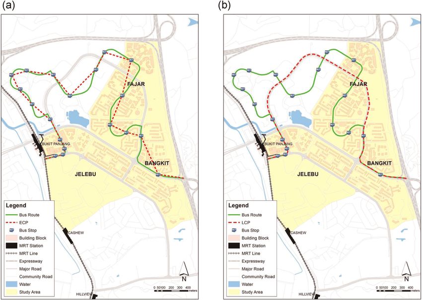
FAN   ET AL.                                                                                                                                 |   571

1     | INTRODUCTION

Public transport is an important service for improving accessibility and addressing congestion in cities
(Anderson, 2014). Better accessibility to public transport results in higher housing price and provides more social
welfare of residents (Chalak et al., 2016; Cohen & Paul, 2007; Holmgren, 2014; Monchambert & De Palma, 2014).
Meanwhile, public transport also constitutes a significant proportion of road transportation, which is one of the
major sources of noise pollution in urban environments (Chui et al., 2004; Monica et al., 2018). Noise pollution has
significant impacts on physical and mental health (Weinhold, 2013; WHO, 2016). Excessive noise also leads to
social issues such as violence and generates economic losses (Cohen & Coughlin, 2008; De Borger & Proost, 2013;
Jamir et al., 2014). With rapid urbanization, the problem of urban noise pollution has been attracting increasingly
more attention from governors, scholars, and the public. However, only a few studies have differentiated the
transportation accessibility benefits and negative environmental externalities for housing price, especially from the
noise of public transport (Chasco & Le Gallo, 2015; Higgins et al., 2019).
      In this paper, we use a natural experiment with a newly launched bus route across a dense residential area in
Singapore to examine the impact of public transport on noise complaints and its influence on housing price. As one
of the world's most densely populated city‐states, Singapore has always faced a severe issue of urban noise
pollution (Lam et al., 2013). More than 80% of its citizens live in public housing, with short distances between
buildings. Around 70,000 complaints of excessive noise are made to government agencies every year (Wan, 2016).
Our study covers the entire 2032 noise complaint records from 142 public housing blocks in three planning
subzones of the Bukit Panjang area in Northwest Singapore from March 2010 to February 2018.
      One of the major challenges for past studies on noise pollution and housing is the lack of real‐time mea-
surement of noise pollution at the building level (Friedt & Cohen, 2020; Segura‐Garcia et al., 2014). To overcome
this challenge, we propose a novel sentiment analysis method to study residents' perception of noise pollution from
their noise complaints.1 Our sentiment analysis method has two advantages: First, government agencies in many
major cities worldwide encourage the residents to report noise incidents, so the database of noise complaint
records naturally exists, such as the Noise Complaints Open Data in New York City. In other words, this method is
not only applicable in Singapore, but also externally valid. Second, our sentiment analysis method captures the
subjective perceptions of noise pollution, which is found to better explain the impact of noise on housing price than
the objective measurements (Boyle & Kiel, 2001; Chasco & Le Gallo, 2013, 2015). Different from past studies using
surveys (Weinhold, 2013), this method captures a quasi‐real‐time measurement of the noise sentiment intensity
and is powerful for baselining the subjectivity of individual responses.
      Another major challenge in past studies is the problem of endogeneity due to omitted variables (Cropper &
Gordon, 1991; Higgins et al., 2018). Singapore's public housing and the public bus enhancement program provides
an ideal context to address the endogeneity problem. Our study area is a representative public housing satellite
town in Singapore. The buildings were almost all constructed during the period when the town was initially
planned, and few further developments have been carried out after that. Public housing blocks, which accom-
modate more than 80% of Singapore residents, have uniform building plans, room layouts, and construction
materials. Demographics such as nationality and ethnicity are controlled for to be evenly distributed based on the
nation's “Ethnic Integration Policy and Permanent Resident Quota” system. As part of Singapore's public bus
enhancement program, a new regional bus service, Route no. 972, was launched in November 2013, and no other
bus routes were introduced in this region during the same period. This allows us to apply a difference‐in‐
differences (DID) strategy to examine the causal noise impact from the launch of the bus service.

1
This sentiment analysis method originates in the field of natural language processing (NLP). SentimentR, which is based on a sentiment dictionary
containing approximately 6800 ranked positive and negative sentiment words, is used in this study (Hu and Liu, 2004; Lam, 2016; Rinker, 2016). Details
of the toolkit are discussed in Appendix A.
572 | FAN ET AL.
In addition, following the strategy of Faber (2014) and Jedwab et al. (2017), we use the hypothetical least cost
route as the instrumental variable (IV) to consistently estimate the causal effect of the new bus on noise com-
plaints. The main IV in the estimation is the Euclidean cost path (ECP), which is the shortest linear distance
connecting all of the bus stops along the bus service route. The other IV used in the robustness check is the least
cost path (LCP), which is the shortest driving route connecting the points at which the bus enters and exits the
study area. Furthermore, to alleviate the concern that unobserved changes in accessibility may correlate with both
the noise sentiment and housing price, we include an explicit control for the change in accessibility before and after
the new bus service when we estimate the impact of noise on housing price.
Our empirical results reveal that at an individual level, the new bus service has worsened the sentiment of
noise complaints from residents living near the bus route (within 100 m) by 10.9 percentage points compared to
those living between 100 and 200 m. If the distance between the housing unit and the bus route decreases by
100 m, the sentiment increases by 9.5 percentage points. These results remain robust if we change the cut‐off
distance to 90 or 110 m, include controls for the noise sentiment in the previous year and the complaint time, use
aggregated sentiment scores at building level, or use alternative theoretically shortest paths as IVs.
The adverse effect also exhibits heterogeneity across floor height and distance to bus stops. For units on the
1st–4th floors and on 9th floor or above, this adverse effect is not statistically significant, probably due to noise
insulation infrastructure on the ground and attenuation of noise on higher floors. On medium floors (5th–8th levels),
however, this adverse effect has doubled in comparison with the average: Living near the bus route (within 100 m)
increases the sentiment by 21.4 percentage points, and a decrease of distance by 100 m increases the sentiment by
24.3 percentage points. The noise effect from the new bus has also shown a larger magnitude on buildings closer to bus
stops, which implies that the introduction of visitors is a major source of noise annoyance.
Finally, we conduct cost and benefit analysis on the impact of public transport on housing price, using resale
transaction data in the study area from 2010 to 2018. By explicitly controlling for the change in accessibility before
and after the new bus, we find that an increase of 1 scale point in noise sentiment is associated with a 3% decrease
in housing price. This implies that, for properties closer to the bus route by 100 m, noise generated by buses leads
to an implicit 0.29% decrease in property value. Using the same transaction data, we also find that, after the new
bus service launches, the prices of properties closer to the bus route by 100 m has increased by 1.34%. Therefore,
our empirical results estimate that over 17.79% of the benefit from improved accessibility brought by the new bus
is offset by the negative externality from its noise pollution.
Our paper contributes to the literature from both conceptual and methodological perspectives. First, we
isolate the negative impact of noise pollution on housing price apart from the accessibility convenience by
launching a new public bus route. It is closely related to the studies of transportation and land use policies for the
transit‐oriented developments (TOD) and for addressing the last‐mile connectivity issue, which is trending not only
in Singapore but also in many other congested cities worldwide (Xie et al., 2010). Improving the accessibility to the
mass public transport involves a significant amount of government investment, while the associated increases in
land values are also expected to sustain the future TOD. Prior literature intensively examines the overall impact of
public transport on housing price (Baum‐Snow & Kahn, 2000; McMillen & McDonald, 2004; Xu et al., 2015), but a
few studies present empirical evidence on cost‐benefit analysis considering the environmental externalities
(Chasco & Le Gallo, 2015; Higgins et al., 2019), possibly because of the costly real‐time measures of noise intensity
and the complexity of the public transport system. Taking advantage of the clean setting of the public bus system in
Singapore's context, we advance current understanding by weighing the advantages and disadvantages of public
transport for housing price. It thus provides empirical evidence for policy makers to minimize the noise exposure in
TOD and maximize the land values.
Second, as Segura‐Garcia et al. (2014) document, current noise map data in the major cities worldwide are
estimations based on sparse measurements and mathematical propagation models, while measuring noise at the
building level in the dense urban environments is costly. We propose a novel methodology to measure the quasi
real‐time noise sentiment at finer detailed level using the noise complaints data, which naturally exists with theFAN ET AL. | 573
government agencies in many major cities (Friedt & Cohen, 2020). In addition, different from measuring noise
incidents by counting frequency through surveys (Tamura et al., 2017; Weinhold, 2013), our methodology
of sentiment analysis also contributes to the literature on understanding residential noise pollution based on
subjective perception, which is proved to show a pattern that is complementary to that in previous literature
(Boyle & Kiel, 2001; Chasco & Le Gallo, 2013; Dzhambov & Dimitrova, 2014).
The rest of the paper is structured as follows. Section 2 reviews the literature and Section 3 introduces the
institutional background. Section 4 presents the empirical specifications, and Section 5 describes the data. Results
are summarized in Section 6, followed by cost‐benefit analysis in Section 7 and Section 8 concludes.
2 | LITERATURE REVIEW
Noise pollution is harmful for human life and activities. According to the WHO, noise exposure is responsible for a
wide range of negative public health issues, such as heart disease, cognitive impairment in children, and stress‐
related mental health risks (WHO, 2016). Exposure to residential road traffic noise is also associated with a higher
risk of diabetes and cardiovascular disease (Münzel et al., 2018; Sørensen et al., 2013). From a social perspective,
community noise pollution increases violent behavior and crime rates and lowers the birth rate and newborn
weights (Jamir et al., 2014; Nieuwenhuijsen et al., 2017). Total socioeconomic loss from road noise pollution in the
UK is similar to the loss from road accidents, and it exceeds the loss from climate change (DEFRA, 2013).
It has been widely acknowledged that better accessibility to public transport results in higher housing price and the
intensification of its service increases the social welfare of residents (Chalak et al., 2016; Cohen & Paul, 2007;
Holmgren, 2014; Monchambert & De Palma, 2014). At the individual level, better accessibility enables participation in
social activities and is associated with positive health outcomes (De Vos et al., 2013; Lucas, 2012). However, the
elevation of service frequency also introduces traffic noise, possibly aggravates environmental pollution (Bilger &
Carrieri, 2013; Nega et al., 2013), and imposes negative externalities on housing price (Ossokina & Verweij, 2015).
Cohen and Coughlin (2008) find that houses under the interruption of airport noise sell for 20.8% less, and the spatial
spill‐over effect magnifies this negative price impact. Chasco and Le Gallo (2015) estimate the households' willingness
to pay for properties with less noise, using the households' subjective perceptions of noise from the census data. Diao
et al. (2016) document that the removal of train noise externalities increases housing prices in the affected area by
13.7%. Higgins et al. (2019) find the accessibility benefits of the new highways are offset by the environmental costs of
air pollution, specifically for the housing units with high accessibility and high exposure to pollution. However, there still
lacks empirical studies about the accessibility benefit and noise cost of public bus, which is one of the common solutions
to address the trending last‐mile connectivity issues in many global cities (Xie et al., 2010).
The real‐time measurement of noise can be very costly at individual building levels in the dense urban environments
(Segura‐Garcia et al., 2014), which has been a major challenge for past studies. Although several cities around the world
are providing the city‐level noise maps,2 only sparse measurements of noise samples at the district or regional level are
taken, and noise contours are estimated using propagation models (Mircea et al., 2008; Swoboda et al., 2015). To
overcome this challenge, one branch of research focuses on improving noise‐measurement instruments or building
empirical mathematical models to simulate real‐time sound environments and noise distribution (Alam et al., 2010; Mak
et al., 2010; Rana et al., 2010). However, these studies usually cover a limited number of buildings and the results may not
be generalized. Other studies propose to use in‐house surveys to construct residents' noise perception index as a proxy
for actual noise levels (Brown & Lam, 1987; Jakovljevic et al., 2009; Park et al., 2016). Nevertheless, the survey method
suffers from a number of drawbacks, such as memory error and retrospective bias in responses (Taylor et al., 2013).
Furthermore, most previous studies in this stream focus on the frequency of troublesome cases, possibly because it is
2
Examples of the city‐level noise maps include the US National Transportation Noise Map (https://www.transportation.gov/highlights/national-
transportation-noise-map), and the London Road Traffic Noise Map (http://www.londonnoisemap.com/).574 | FAN ET AL.
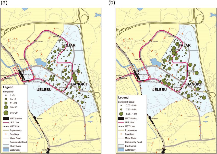
F I G U R E 1 Map of noise complaint frequency and sentiment severity in Singapore's Bukit Panjang Area during
2010‐2018. (a) Complaint frequency and (b) sentiment severity [Color figure can be viewed at wileyonlinelibrary.com]
difficult to address subjectivity when measuring the severity of noise incidents (Weinhold, 2013). Recent studies also
exploit the frequency of residents' noise complaints as an alternative measure of noise pollution (Friedt & Cohen, 2020).
However, incidence and intensity are two distinct dimensions, and are expected to have different patterns (Figure 1).
The concept of sentiment analysis that we use to measure noise annoyance in this study was introduced in the
early 2000s, when computer scientists tried to extract polarized opinions (either positive or negative) from
customer reviews of commercial goods or movies (Pang et al., 2002; Turney, 2002). It has since been applied in
various empirical studies involving human perceptions (Cambria et al., 2013). Tetlock (2007) finds that the fre-
quency of negative words in Wall Street Journal articles predicts stock returns, and Garcia (2013) finds that this
predictive power is stronger during recessions. Using search results from Google, Zheng et al. (2016) conclude that
investor confidence is a determinant of China's housing price.
In addition, past literature has also discussed the challenge that unobserved factors may be simultaneously
associated with public transport and the perception of urban noise, which undermines the reliability of empirical
results (Cropper & Gordon, 1991; Higgins et al., 2018). For instance, the intensification of public transport services
may be an ex post action by the government to address the growing population in the area, while the higher
resident density also induces more noise. Residents' unobserved personal attributes may also threaten the esti-
mation, as residents who are sensitive to noise are likely to choose quieter locations and are less tolerant of a
sudden increase in noise. One of the main empirical approaches to address this challenge is to develop IVs that
are highly correlated with the actual route of the transportation service but are intended to affect noise
output only through this correlation (Redding & Turner, 2015). In the literature, commonly applied instruments
include the initially planned route (Baum‐Snow, 2007; Donaldson, 2018; Michaels et al., 2012), the historical routeFAN ET AL. | 575
(Duranton & Turner, 2011; Hsu & Zhang, 2014; Martincus et al., 2017), and other related hypothetical routes
(Banerjee et al., 2020; Faber, 2014; Jedwab et al., 2017; Tsivanidis, 2019).
3 | INSTITU TIONAL B ACKGROUND
3.1 | Public housing and residential noise in Singapore
The issue of residential noise pollution is serious in densely populated modern cities such as Singapore. According
to the Straits Times, “over 7,000 residents are living in each square kilometer of land in Singapore,” and “more than
85 percent of its residents live in the nation's public housing flats with very close distance to roads, constructions
or other building blocks.” Around 70,000 complaints are made to various government agencies each year about
excessive noise in Singapore (Wan, 2016). To manage noise pollution in public housing, the local public housing
authority—the Housing Development Board (HDB)—has promoted the Neighborliness Campaign among residents,
which encourages them to respect the neighborhood by avoiding producing excessive noise. The National
Environment Agency (NEA) has also established regulations to control for noise origins, such as setting maximum
permissible noise levels for factories and construction work, a no‐work rule during certain periods of the day, and
maximum noise emission limits for air conditioning and mechanical ventilation systems in buildings. In case of
excessive noise, residents can also call or email the hotlines located in individual town centers.
Public housing in Singapore provides an ideal setting to study urban residential noise pollution. As one of the
world's most successful public housing schemes, new units are sold to citizens and permanent residents by the
government at prices much lower than the market price. Owners are also allowed to resell their public housing
units to other eligible buyers at the market price. On the one hand, residential noise pollution in public housing is
much more serious than in private estates, which leads to policy incentives for social equality. Due to concerns
about land and construction cost, most public housing is densely constructed using economical materials, which
provide limited performance in noise insulation. Since residents living in public housing have stronger demand
for public transport, most public housing is located closer to transportation hubs or major roads. This leads to
more exposure to traffic noise. On the other hand, different building and urban attributes, such as building
typology and floor level, will have significant noisescape influence (Lam et al., 2013; Mak et al., 2010). This makes
it challenging to control for these noise‐related variables in a complex urban context. In Singapore, however,
public housing has undergone around four waves of morphological changes, and the buildings constructed in
each era have uniform morphology (Pow, 2009). This makes it feasible to largely exclude the impact from variant
morphology in this study.
3.2 | Study area and the new bus service
Our study covers 142 HDB blocks in the subzones of Fajar, Jelebu, and Bungkit of Bukit Panjang District in
Northwest Singapore, which accommodate around 100 households per building. The district of Bukit Panjang is
one of the oldest residential suburban towns in Singapore. To meet demand stemming from the population surge
after the nation's independence, the development of public housing in the town began in the early 1980s. Most of
the HDB development was completed by the mid‐1990s, and only a few new residential projects or redevelop-
ments have been completed since then. As a result, the morphology of HDB blocks in the study area mostly follows
the two standard prototypes for HDB buildings in that generation: 132 Slab Blocks and 8 Point Blocks (Appendix
Figure B1). Slab Blocks are between 12 and 14 stories, and Point Blocks are all 25 stories. Only two blocks
have been redeveloped in recent years, for which a new building typology was adopted. HDB buildings from the
same generation are also constructed using standard materials, and layouts of the units and the number of rooms576 | FAN ET AL.
are almost the same. Like any other public housing in Singapore, regular repainting and upgrading programs are
also conducted in this district every 5–7 years. Therefore, the maintenance of these buildings is also kept at a
similar level.
Sales of HDB blocks are restricted to Singapore citizens or permanent residents, and there is a quota for
noncitizen owners in each building. The nation's Ethnic Integration Policy requires that the proportion of
owners' ethnicity in each individual building strictly follows the national average proportions of Singapore's
three major races (Chinese, Malay, and Indian). If the number of owners from one race hits the threshold,
owners from this race can only sell the unit to buyers of the same race. Therefore, on the aggregate block level,
the distributions of residents' ethnicities are relatively uniform. According to the population surveys in 2010
and 2015, the distributions of residents' gender and age groups are also relatively stable in our study area
(DOS, 2019).
The road network in the area follows a typical town planning hierarchy in Singapore. The north and east sides
of the site are enclosed by the two highest standard expressways, and on the other side of the expressways are
reserved forest land with limited urban development. One major road (Bukit Panjang Road) cuts through the site to
connect with the expressways, and a secondary ring road forms a loop to direct traffic to the major road. All other
minor roads in the community are connected to the ring road loop. Since 1999, there has been a light rail train
(LRT) line looping in the district, which connects to the nearby Choa Chu Kang mass rapid transit (MRT) station on
the North‐East Line. The Bukit Panjang MRT station—the terminal station of the Downtown Line—also connects to
this LRT line in the district; it started operations on December 27, 2015.
Like many other major cities worldwide, the Singapore government aims to address the trending last‐mile
connectivity issue in the city by improving the service coverage and frequency of its public buses (Xie et al., 2010).
Public buses are the most frequently used transportation mode (41.3%) by the population traveling to work in
Singapore (GHS, 2015). Singapore's Ministry of Transport aims to increase the peak‐hour public transport mode
share to 75% by 2030, and it launched the Bus Service Enhancement Programme (BSEP) to expand the bus fleet by
35% before 2017.
As part of the BSEP program, a new regional bus service, Route no. 972, was launched in November 2013 in
our study area (Figure 2). It operates daily from 6 a.m. to 11:30 p.m. The service frequency is every 4–5 min during
the peak hours and every 8–10 min during the nonpeak hours. Our study site has an area of 1.2 km2, and the
segment of the bus route in our site is over 2.5 km long with six bus stops. The bus stops are sequentially allocated
along the road at intervals of about 300–400 m. Unlike buses intended to connect the community with other
districts in the city, this bus is designed to improve last‐mile connectivity within the community. Therefore, instead
of driving on the fastest path along major roads, this bus zigzags along minor community roads to ensure that most
of the blocks are within 200 m of its service cover. Apart from Route no. 972, no other buses were introduced
along a similar route during our study period, and the service frequencies of existing buses have not been changed
since the introduction of bus no. 972. The new route was announced only 11 days before launching the service, and
there were no other government documents disclosing the new bus route in our study area before the an-
nouncement. Therefore, the anticipation effect is likely minimal.
4 | E MP I R I CA L ST R AT EG Y
A standard DID strategy estimates the net impact of proximity to new public transport services on housing
prices (Diao et al., 2017). However, it is not able to differentiate the benefit of accessibility and the cost of
environmental externalities, because both the benefit and the cost correlate with the closeness to public
transport. Therefore, we apply a two‐step strategy to specifically estimate the negative impact of noise from
public transport on housing price. First, we apply a DID strategy to estimate the impact of closeness to the new
bus route on noise sentiment. Second, we estimate the impact of lagged noise sentiment on subsequentFAN ET AL. | 577
F I G U R E 2 Actual service route of bus no. 972 and the constructed theoretically least cost path of ECP and
LCP (a) ECP and actual bus route (b) LCP and actual bus route. ECP, Euclidean cost path; LCP, least cost path
[Color figure can be viewed at wileyonlinelibrary.com]
housing price, by explicitly controlling for the change in accessibility. Combining the results from the two
steps, we interpolate the negative impact of closeness to the bus route on housing price due to the noise.
Finally, we compare the net impact of public transport on housing price and its negative impact due to noise,
and we estimate how much benefit of accessibility is offset by the noise externalities. The following part of this
section explains our empirical specifications in detail.
4.1 | Public bus and noise complaints: Baseline estimation
The baseline estimation uses complaint records from March 2010 to February 2018 with intact floor and unit
information. The following DID specification is applied:
SIijt = β1 Neari + β2 Launcht + β3 Launcht ∗Neari + Xi′ θ + U′j μ + φt + ωi + εijt, (1)
where SIijt is the sentiment score from a complaint made at time t by a resident living in building i and unit j .
Launcht is a dummy variable, and it is one if complaint time t is later than the launch of bus service. Otherwise,
it equals to zero. Neari is a dummy variable indicating whether block i is within 100 m of the actual bus route.
In other words, the treatment group includes buildings within 100 m and the control group includes
buildings within 100–200 m. Therefore, the coefficient of the interaction between Launcht and Neari is the
estimate of the causal impact of the new bus route on noise complaints. We use proximity to the bus route578 | FAN ET AL.
rather than the closest bus stop in our identification strategy, because noise can be generated both from bus
stops and along the road (Diao et al., 2016). Since the bus stops are located along the bus route, using
this strategy also facilitates the investigation of the heterogeneous impact across distance to bus stops
(Appendix Figure B2).
In addition, we further allow variation in the distance from each building to the new bus as the measure for the
linear attenuation of noise pollution. We specify Distancei , a continuous variable as an alternative to Neari , in
Equation (2).
SIijt = β1 Distancei + β2 Launcht + β3 Launcht ∗Distancei + Xi′ θ + U′j μ + φt + ωi + εijt. (2)
Xi is a vector controlling for building i 's physical properties, which include the morphology of the building
(slab block, point block, or new HDB block), age of the block, existence of residential community (RC) centers,
and its distance to MRT/LRT stations, the LRT viaduct line, bus stops, expressways, and major roads. These
factors are common sources of residential noise. Uj is the vector controlling for unit‐specific properties,
including the floor level and its squared form, and the gender of the complainant. φt is the year times month
fixed effect, and ωi is the block fixed effect. εijt is the error term. Standard errors are clustered by building
blocks.
4.2 | Hypothetical LCP
The ordinary least square (OLS) estimates from Equations (1) and (2) are likely to be biased if the design of the bus
service route is not random. To address this concern, we construct a hypothetical least cost bus route, and use the
distance to the least cost route as the instrumental variable for distance to the actual bus route, following the IV
construction strategies from Faber (2014) and Jedwab et al. (2017). We define two such theoretically shortest
paths. The first one, following the strategy of Faber (2014), assumes that the original bus stops along the service
route are the fixed nodes and uses Euclidean straight lines to connect these nodes as the shortest path. This path is
denoted as the ECP and is presented in Figure 2a. In the second construction, we consider actual travel time as the
cost indicator. By fixing only the bus's entrance and exit points in the site, we use Google Map to calculate the
shortest‐time commuting path connecting these two points. This path is denoted as the LCP and is drawn in
Figure 2b. Distances from buildings to these paths are calculated using ArcGIS. We use the ECP as the main IV and
include the LCP in the robustness check.
These theoretically shortest paths are valid instruments because of their relevance and exclusion restrictions
(Redding & Turner, 2015). On one hand, the actual bus route deviates from the theoretically shortest route to
cover more residential areas, but it is not likely to deviate too far from the theoretical path. This is because bus
service must also compete with alternative travel modes, such as trains and private driving, and must take
passengers' total commuting time into consideration. Thus, the actual bus route is expected to be highly correlated
with the theoretically shortest route.
On the other hand, the theoretical path is considered to be uncorrelated with noise annoyance beyond its
correlation with the actual bus service. In particular, two unobserved trends may be present that potentially
threaten our estimations. First, the government may design the new bus route to serve some specific areas
(e.g., buildings with higher population density), where there might be more neighborhood noise. The theoretically
shortest paths are not expected to correlate with these unobserved trends in neighborhood features along the
actual bus route. Second, residents who are more sensitive to noise may self‐sort into units that are farther from
streets. Nevertheless, our ECP instrument is a hypothetical path, so it is unlikely to correlate with any residential
sorting trends along the real roads.FAN ET AL. | 579
4.3 | Noise complaints and housing price
Further, we examine the impact of residents' noise sentiment on housing price. We test this effect from the yearly
aggregated noise sentiment in each block.3 The empirical specification is as follows:
log (Priceijt ) = βSIi, t − 1 + Xi′ θ + U′j μ + λMt + φt + ωi + εijt, (3)
where log (Priceijt ) is the log form of the transaction price for unit j in block i sold at time t . SIi, t − 1 is the average
noise sentiment in block i during the 12 months before transaction time t . The coefficient β is thus the estimate
of the effect of the noise sentiment on housing price. Xi is the same vector controlling for characteristics of
building block i as in Equations (1) and (2). Uj controls the properties of the housing unit, including its size and
floor level. Mt represents the macroeconomic index and equals the prime lending rate for bank mortgages at
time t . φt is year times quarter fixed effect, while ωi is the block fixed effect. εijt denotes the error term.
Standard errors are clustered by building blocks.
The OLS estimate of coefficient β in Equation (3) is likely biased upward due to endogeneity and may serve
as an upper bound of the true negative effect of noise pollution on housing price (i.e., a lower bound in mag-
nitude). It is because the variable of noise sentiment (SIi, t − 1 ) may positively pick up the benefit brought by
unobserved factors, such as the changes in accessibility. To estimate the exact economic costs of noise pollution
on housing price, we further include an explicit control for accessibility before and after the launch of bus no.
972. Specifically, we use distance to the nearest bus stop connecting to the Central Business District (CBD) of
Singapore as a proxy for change in accessibility. As illustrated in Appendix Figure B3a, the new bus route
(no. 972), which zigzags within the RC, aims to solve the problem of last‐mile connectivity to the CBD. Before the
launch of bus no. 972, the only bus connecting the site and the CBD was route no. 190, which operates along a
major road (Appendix Figure B3b). Therefore, before the launch of the new bus route, the nearest bus stop
connecting to the CBD only lies on the route of no. 190. After the treatment, it will be on either bus route no.
190 or bus route no. 972.4
5 | DATA
In Singapore, residents in public housing report their noise complaints to the local government through hotlines,
email, or other written notices. These records are then centralized by local Community Development Councils
(CDC) for further action. The data in our study are provided by the local government and cover all noise complaints
made by HDB residents in the study area from March 2010 to February 2018. We collected the entire 2032
records on noise complaints in all 142 buildings. The number of complaints per building at the 25th percentile, the
median, and the 75th percentile are 6, 11.5, and 17, respectively. For each complaint, the incident date, time, and
complaint content are recorded by the agency that receives the complaint.
A cleansing process is applied before calculation of sentiment scores. Specifically, we manually corrected the
grammatical errors and typos in the complaint records. In addition, when complaint data were recorded, the registrar
used a number of abbreviations, such as “plz” for “please.” These abbreviations are also manually revised. The sentiment
score of each individual noise report is then calculated by running the SentimentR tool on the cleaned complaint
contents. Results are winsorized to the top and bottom 1% of the distribution to remove the impact of outliers. This is
followed by a normalization of scores to the range from zero to one, which represents the most low‐key and the most
severe emotions, respectively.
3
Noise compliant records are too scarce to map onto individual housing transactions.
4
After the treatment, 63 out of the 142 blocks in our study area have the nearest bus stop connecting to the CBD on the new route no. 972.580 | FAN ET AL.
A subset of 593 records in the database contain the complainant's full unit number and floor.5 The maximum
distance from the building to the new bus route is 198.5 m. There are 328 complaints within 100 to 200 m of the bus
route (the control group), and 265 complaints within the 100‐m boundary (the treatment group). The parallel trend
between treatment group and control group is also verified (Appendix Figure B4). The average difference between the
distance from the building to the ECP and the distance from the building to the bus route is 46 m, which equals 41% of
the average distance to bus route. The average difference between the distance to the LCP and the distance to the bus
route is 75 m, which equals 67% of the average distance to bus route. Distributions on demographics and the physical
features of buildings are consistent with the standard for Singapore's public housing (GHS, 2015). When the com-
plainant calls the hotline, the registrar will usually record the complainant's title (Mr., Ms., etc.) so that information on
their gender can be obtained, which yields 527 records from 96 buildings. We use these 527 records as our main
sample in the baseline regressions. There are 227 cases before the launch of the bus and 300 cases after. The gender
distribution remains stable in the pretreatment (46.70%) and posttreatment periods (46.67%). In total, 80 out of the
96 buildings (83.3%) have complaint records both before and after the new bus service, and the geographic dis-
tributions of buildings with noise complaints are similar before and after launching the new bus (Appendix Figure B5).
Geo‐referenced information on the site's administrative boundary is obtained from the Singapore government's
online public data portal, while information on building blocks, road networks, MRT and LRT lines, and bus stops are
downloaded from OpenStreetMap. We also code the morphological classification of the buildings and the locations of
RC centers. The list of shopping centers in the study area is from the OneMap of Singapore's Urban Redevelopment
Authority. The age of each building block is from the HDB website. The distance from each building block to roads, bus
stations, or other public facilities is calculated using ArcGIS.6 The LRT line in our study area operates on a viaduct,
which causes noise exposure, so the distance from buildings to the viaduct is also calculated. Table 1 presents summary
statistics for these complaint cases. The average distances to train stations, bus stops, and expressways are 212.5,
120.2, and 428.1 m, respectively.
Data on housing transactions, including transaction price, date, floor, and size of the unit, are also obtained from
the government's online public data portal. In our study period, there are 1450 resale transactions from 131 out of
142 buildings in our study area, and the information is also summarized in Table 1. The averaged transacted housing
price is 375,207 SGD, which is equivalent to approximately 278,365 USD. The dwelling size is 104 m2 on average, with
a mean floor level of 6.7. This is similar to the national average statistics, so our sample is also representative of public
housing transactions in Singapore (GHS, 2015). Of these transactions, 893 can be matched with noise complaints in the
same building 12 months before the transaction date, and we use them as our regression sample. The prime lending
rate for bank mortgages is directly retrieved from the Monetary Authority of Singapore (MAS).
6 | E F F E C T S O F P U B L I C T R A N S P O R T O N N O I S E C O M PL A I N T S
6.1 | Baseline estimation results
Table 2 reports first‐stage IV regression results for the effects of bus routes on noise complaints at the individual level.
Columns (1) and (2) examine the binary indicator of closeness to the bus route, as specified in Equation (1), using ECP and
the combination of ECP and LCP as the instrument(s), respectively. Columns (3) and (4) include the numerical distance to
the bus route instead, as specified in Equation (2), and also apply ECP and the combination of ECP and LCP as the
5
We also conduct the robustness test at building level to address the issue of missing unit information for individual cases.
6
We use distance from the main entrance of building to the road as the proxy for the distance from each unit to the road, due to a lack of information on
the floor plan. Since most of the buildings in our study area are slab type and a majority of units are located along the corridor parallel to the road, the
distances from the units to the road are roughly the same within buildings. Linear distance to roads is used because noise propagates linearly. We also use
the linear distance to amenities as the proxy for measuring walking accessibility, because the first floors of Singapore's public housing buildings are empty
(i.e., the “void deck”), and pedestrians are free to pass through the buildings.FAN
TABLE 1 Summary statistics of noise complaints and housing transactions
Diff ((5)–(8))
ET AL.
Total Near = 0 (100–200 m) Near = 1 (within 100 m)
N Mean SD N Mean SD N Mean SD t‐test
(1) (2) (3) (4) (5) (6) (7) (8) (9) (10)
Noise sentiment 593 0.409 0.165 328 0.416 0.170 265 0.399 0.159 0.017
Distance (100 m) 593 1.111 0.493 328 1.483 0.317 265 0.650 0.187 0.833***
LCP (100 m) 593 1.737 1.323 328 2.136 1.349 265 1.243 1.108 0.893***
ECP (100 m) 593 1.068 0.794 328 1.516 0.649 265 0.514 0.578 1.001***
Launch (after = 1) 593 0.575 0.495 328 0.512 0.501 265 0.653 0.477 −0.141***
Near (within 100 m = 1) 593 0.447 0.498
RC center (with = 1) 593 0.069 0.254 328 0.0671 0.251 265 0.072 0.258 −0.005
Building age 593 29.022 2.267 328 28.902 2.584 265 29.170 1.794 −0.267
Floor level 593 6.408 3.960 328 6.479 3.976 265 6.321 3.946 0.158
Morphology 593 2.926 0.293 328 2.878 0.371 265 2.985 0.122 −0.107***
Gender (Male = 1) 527 0.467 0.499 300 0.503 0.501 227 0.419 0.494 0.085*
To train station (100 m) 593 2.125 1.155 328 2.435 1.224 265 1.741 0.933 0.693***
To LRT line (100 m) 593 1.531 1.154 328 1.884 1.155 265 1.093 0.994 0.790***
To bus stop (100 m) 593 1.202 0.501 328 1.335 0.548 265 1.038 0.377 0.233***
To expressway (100 m) 593 4.281 2.030 328 4.553 2.357 265 3.945 1.468 0.608***
To major road (100 m) 593 1.217 0.816 328 1.359 0.758 265 1.041 0.851 0.318***
To shopping center (100 m) 593 5.302 2.863 328 5.181 3,154 265 5.452 2.467 −0.271
Price (thousand SGD) 1450 375.207 73.564 1003 364.924 69.114 447 398.282 77.968 −33.359***
(Continues)
|
581Diff ((5)–(8))
582
Total Near = 0 (100–200 m) Near = 1 (within 100 m)
|
N Mean SD N Mean SD N Mean SD t‐test
(1) (2) (3) (4) (5) (6) (7) (8) (9) (10)
Floor 1450 6.710 3.630 1003 6.671 3.588 447 6.799 3.724 −0.128
2
Area (m ) 1450 103.595 20.399 1003 99.984 19.56 447 111.696 19.928 −11.712***
Note: Morphology equals to 1 if the block follows the new generation building layout, 2 if it follows the point block layout, or 3 if it follows the slab block layout.
Abbreviations: ECP, Euclidean cost path; LCP, least cost path; LRT, light rail train.
*p < 0.1.
**p < 0.05.
***p < 0.01.
FAN
ET AL.FAN ET AL. | 583
TABLE 2 First‐stage IV estimation results of the effects of bus route on noise complaints at individual level
(1) (2) (3) (4)
Launch Launch Launch × Launch ×
× Near × Near Distance Distance
Launch × ECP −0.3653*** −0.3306*** 0.4184*** 0.4025***
(0.0546) (0.0615) (0.0520) (0.0602)
ECP 0.0190 0.0367 −0.0070 −0.0491
(0.0419) (0.0451) (0.0364) (0.0395)
Launch × LCP −0.0787** 0.0491
(0.0360) (0.0352)
LCP −0.0790 0.1558**
(0.0651) (0.0644)
Launch 0.7781*** 0.8410*** 0.8278*** 0.7932***
(0.2049) (0.2067) (0.2051) (0.2057)
Building age −0.0040 −0.0023 −0.0117 −0.0158
(0.0119) (0.0119) (0.0104) (0.0102)
Floor 0.0007 −0.0000 0.0029 0.0033
(0.0123) (0.0126) (0.0102) (0.0105)
Floor squared 0.0005 0.0005 −0.0008 −0.0008
(0.0007) (0.0007) (0.0006) (0.0006)
Point block 0.0401 0.0605 0.3776** 0.3339**
(0.1951) (0.1908) (0.1789) (0.1692)
Slab block 0.0943 0.1315 0.1492 0.0789
(0.1448) (0.1457) (0.1397) (0.1330)
Male −0.0402 −0.0405 0.0156 0.0149
(0.0299) (0.0286) (0.0239) (0.0228)
RC center −0.0094 −0.0105 −0.0135 −0.0083
(0.0796) (0.0803) (0.0684) (0.0692)
Block and time fixed effect Y Y Y Y
First‐stage F‐Stats 22.69 26.81 32.67 38.07
J‐Statistics (p value) 0.2787 0.2235
Observations 527 527 527 527
Note: Columns (1) and (2) report results for the binary closeness indicator. Columns (3) and (4) report results for the
continuous distance variable. Columns (1) and (3) use the ECP, the Euclidean straight lines connecting bus stops, as the
instrument. Columns (2) and (4) use both ECP and LCP, the least travel time path, as the instrument. Unreported control
variables include distance to train stations, LRT viaduct line, bus stops, expressways, major roads, and shopping centers.
Standard errors are clustered by building blocks. Robust standard errors in parentheses.
Abbreviations: ECP, Euclidean cost path; LCP, least cost path.
*p < 0.1.
**p < 0.05.
***p < 0.01.584 | FAN ET AL.
T A B L E 3 OLS and second‐stage IV estimation results of the effects of bus route on noise complaints at
individual level
Noise sentiment
(1) (2) (3) (4) (5) (6)
OLS ECP IV Both IVs OLS ECP IV Both IVs
Launch × Near 0.0496 0.1090** 0.1118**
(0.0324) (0.0459) (0.0437)
Near −0.0136 −0.0105 −0.0300
(0.0303) (0.0529) (0.0476)
Launch × Distance −0.0405 −0.0953** −0.0965**
(0.0338) (0.0430) (0.0422)
Distance 0.0074 0.0125 0.0301
(0.0328) (0.0462) (0.0423)
Launch −0.1123 −0.1330 −0.1365 −0.0400 0.0319 0.0333
(0.1217) (0.1069) (0.1054) (0.1167) (0.1140) (0.1114)
Building age −0.0016 −0.0011 −0.0015 −0.0019 −0.0024 −0.0022
(0.0048) (0.0044) (0.0044) (0.0048) (0.0044) (0.0043)
Floor −0.0130* −0.0126** −0.0128** −0.0128* −0.0122* −0.0125**
(0.0070) (0.0063) (0.0063) (0.0071) (0.0063) (0.0063)
Floor squared 0.0008* 0.0007* 0.0007* 0.0008* 0.0007* 0.0007*
(0.0004) (0.0004) (0.0004) (0.0004) (0.0004) (0.0004)
Point block −0.0487 −0.0764 −0.0593 −0.0423 −0.0457 −0.0415
(0.0811) (0.0786) (0.0786) (0.0792) (0.0739) (0.0728)
Slab block −0.0429 −0.0675 −0.0505 −0.0409 −0.0484 −0.0393
(0.0543) (0.0549) (0.0554) (0.0508) (0.0475) (0.0480)
Male 0.0181 0.0195 0.0186 0.0171 0.0166 0.0156
(0.0201) (0.0188) (0.0186) (0.0199) (0.0187) (0.0186)
RC center 0.0484* 0.0448* 0.0501** 0.0453* 0.0420* 0.0463*
(0.0269) (0.0251) (0.0251) (0.0260) (0.0236) (0.0239)
Block and time fixed effect Y Y Y Y Y Y
Observations 527 527 527 527 527 527
2
R 0.214 0.203 0.207 0.213 0.206 0.208
Note: Columns (1)–(3) report results for the binary closeness indicator and Columns (4)–(6) report results for the
continuous distance variable. Columns (1) and (4) are OLS estimation results. Columns (2) and (5) use the ECP, the
Euclidean straight lines connecting bus stops, as the instrument. Columns (3) and (6) use both ECP and LCP, the least travel
time path, as the instrument. Unreported control variables include distance to train stations, LRT viaduct line, bus stops,
expressways, major roads, and shopping centers. Standard errors are clustered by building blocks. Robust standard errors
in parentheses.
*p < 0.1.
**p < 0.05.
***p < 0.01.FAN ET AL. | 585
instrument(s), respectively. First‐stage results reveal that both ECP and the combination of ECP and LCP are strongly and
statistically significantly correlated with the actual bus service route, controlling for the physical features, gender of the
complainants, and the fixed effect from time and building. The F‐statistics in all specifications are around 20–30, miti-
gating concerns about weak instruments. For estimations with more instrumental variables than endogenous variables
(Columns (2) and (4)), the J‐statistics for over‐identification test are 0.2787 and 0.2235, respectively.
Table 3 presents OLS and second‐stage IV estimation results. Column (1) presents OLS estimates from
Equation (1), while Columns (2) and (3) display IV estimates using ECP and the combination of ECP and LCP,
respectively. Columns (4)–(6) show corresponding estimates from Equation (2). The OLS estimate is positive,
though with no statistical significance, in Column (1), and it is likely contaminated by unobserved factors. For
example, residents who are less sensitive to noise will choose to live in units closer to roads and will also make less
noise complaints. Therefore, the OLS estimate of the noise effect will be downward biased in magnitude. Using ECP
as an instrument, being close to the bus service route (within 100 m) results in a higher negative sentiment score of
0.109 (Column (2)) and 0.112 (Column (3)) using both ECP and LCP as IVs. Both of the two IV estimates are
statistically significant at the 5% level. Since the sentiment score is normalized to the range of 0 to 1, this indicates
that intensification of public transport services worsens the noise sentiment in surrounding public housing by
approximately 11 percentage points. The continuous distance effect is estimated to be −0.095 (Column (5)) using
ECP as the IV, or −0.097 (Column (6)) using the combined IVs. Both estimates are statistically significant at the
5% level. Consistent with previous findings using a binary indicator of closeness, the distance estimates reveal that
by living closer to road traffic by 100 m, the negative noise sentiment will increase by around 10 percentage points
on average.
One assumption in the interpretations above is that the intensification of the bus service is the only source of
changing noise levels along the bus route. A possible concern about the validity of this assumption is that with the
newly opened bus route, increased bus traffic will change the traffic patterns of other vehicles on the route. For
instance, commuters using private vehicles instead of public buses may choose other routes to avoid congestion.
However, under this scenario, the traffic volume from other vehicles is expected to decrease after the treatment,
and the measured increase in noise sentiment in buildings near the bus route will be smaller than the real increase
due to the new bus. In other words, the real impact of closeness to the new bus service on noise sentiment is likely
larger than our estimates.
6.2 | Robustness checks
We first examine the robustness of our baseline results by setting different cut‐off distances for the treatment and
control groups in the DID estimations. Since the maximum distance to the bus route for buildings in our sample is
198.5 m, we set the cut‐off distance to be 100 m in the baseline estimation to balance sample size in each group. This
100 m boundary for road traffic noise insulation is also supported by the acoustics literature (Avsar & Gonullu, 2005;
Martin & Hothersall, 2002). As robustness checks, we follow the same empirical strategy as Equation (1) but change the
cut‐off distances to 110 or 90 m. The corresponding estimation results are reported in Appendix Table C1. The
estimates are very close to those in our baseline results, for both the magnitude and statistical significance.
Another possible concern about the baseline estimation result is that an individual's sentiment about a new
noise incident is dependent on previous exposure to noise. If the surrounding environment has been noisy for
years, residents may not notice additional noise incidents, while residents living in quiet housing units may be less
tolerant of a sudden increase in the noise level. To alleviate this concern, the average sentiment score of noise
complaints made in the same building with a 1‐year lag is included as an additional control. Results are reported in
Appendix Table C2. The estimates remain robust in magnitude and level of significance.
In addition, the occurrence time of noise incidents may impact the noise sentiment, because residents may
be disrupted more easily at night. Therefore, we use the report time of the noise complaints as a proxy for the occurrence586 | FAN ET AL.
time of the noise incidents and include it as an additional control in the baseline model. Specifically, we denote the
complaints made between 7 p.m. and 7 a.m. as the complaints made at night and denote the rest of the complaints as
the ones made in the daytime. Appendix Table C3 reports the corresponding estimation results. As we expect, it reveals
that complaints made at night have stronger adverse sentiments by around 10 percentage points. Living closer to the bus
route by 100 m is estimated to have stronger noise sentiments by 10.4–10.5 percentage points, and the estimates are
statistically significant at 5% level and 1% level, respectively. This indicates that our baseline estimation results remain
robust.
Moreover, we address potential self‐selection in the complaint samples. At the building level, to ensure that
the composition of the sampled buildings is homogeneous, we conduct a robustness check by including only the
buildings that have complaints both before and after the new bus service. The estimation results are reported in
Appendix Table C4. Our results remain robust. On the individual level, if some residents are sorted to the areas
near the bus route after the new bus service, they are expected to have gained ex ante knowledge of the new
traffic noise when they inspected the houses before movement. Thus, it is possible that these new residents, who
choose to live in a noisy area, report less severe complaints than those original residents who used to live in a quiet
area and are now exposed to more noise. In that case, our estimated impact of closeness to the new bus service on
noise sentiment is likely to provide a lower bound estimate of the true impact. In other words, the magnitude of the
true impact of the new bus service on noise sentiment will be even larger than our estimation.
Further, to address potential selection by excluding individual cases without unit‐level information and po-
tential measurement error in the distance between each unit and the bus route, we further conduct the analysis at
an aggregated building level. Within each building block, the sentiment of complaints in the past 12 months is
averaged to construct the aggregate building‐level sentiment index. In this way, records without full floor, unit, or
demographic information can then be included in the analysis. Specifically, using a 12‐month window before and
after the opening of the new bus route, we investigate the impact of bus service on average noise sentiment within
buildings. This specification follows the empirical strategies applied by Faber (2014):
SIiAfter − SIiBefore = β1 Neari + Xi′ θ + εi, (4)
SIiAfter − SIiBefore = β2 Distancei + Xi′ θ + εi, (5)
where SIiBefore and SIiAfter are the average sentiment scores of noise complaints in block i recorded 12 months before
and after launch of the new bus service. Neari is the dummy variable indicating whether block i is within 100 m of
the actual bus route, and Distancei is the distance from block i to the actual bus route. Xi is the same vector
controlling for building i 's physical properties, as in the individual case‐level estimation. εi is the error term. Like the
case‐level estimation, we use the ECP as IV for Neari and Distancei in the main regressions, and include LCP in the
robustness check.
Appendix Table C6 presents the OLS and IV estimation results of Equations (4) and (5).7 Living in buildings
within 100 m of the bus route has an incremental noise sentiment score of 0.204 (Column (2)) if using ECP as the
IV, while the effect is 0.220 (Column (3)) if using the combined IVs. On the continuous scale, buildings closer to the
bus route by every 100 m present worsened noise annoyance by 13.2 percentage points (Column (5)) using ECP as
the IV, and 14.8 percentage points (Column (6)) using the combined IVs. All of the IV estimates are statistically
significant at conventional levels of significance. Such evidence at an aggregate level is consistent with the
individual‐level pattern, which consolidates the impact of the new bus route on noise complaints.
Lastly, we examine the robustness of our results using two alternative IV strategies. First, our ECP theoretical
path is constructed by connecting the bus stops, so the distance to the ECP is uncorrelated with the potential
sorting of residents along the actual road (Faber, 2014). To alleviate the concern that the locations of the new bus
stops may not be exogenous, we construct an alternative ECP IV by connecting random points along the bus route
7
First‐stage results are presented in Appendix Table C5.You can also read