Reports on progress in physics the complex dynamics of earthquake fault systems: new approaches to forecasting and nowcasting of earthquakes
←
→
Page content transcription
If your browser does not render page correctly, please read the page content below

Reports on Progress in Physics

REVIEW

Reports on progress in physics the complex dynamics of earthquake
fault systems: new approaches to forecasting and nowcasting of
earthquakes
To cite this article: John B Rundle et al 2021 Rep. Prog. Phys. 84 076801

View the article online for updates and enhancements.

                             This content was downloaded from IP address 169.237.222.219 on 28/05/2021 at 18:47
Reports on Progress in Physics

Rep. Prog. Phys. 84 (2021) 076801 (37pp)                                                              https://doi.org/10.1088/1361-6633/abf893

Review

Reports on progress in physics the
complex dynamics of earthquake fault
systems: new approaches to forecasting
and nowcasting of earthquakes
John B Rundle1,2,3,∗ , Seth Stein4 , Andrea Donnellan5 , Donald L Turcotte2 ,
William Klein6 and Cameron Saylor1
1
  Department of Physics and Astronomy, University of California, Davis, CA 95616, United States of
America
2
  Department of Earth & Planetary Sciences, University of California, Davis, CA 95616, United States of
America
3
  Santa Fe Institute, 1399 Hyde Park Rd, Santa Fe, NM 87501, United States of America
4
  Department of Earth and Planetary Sciences and Institute for Policy Research, Northwestern University,
Evanston, IL 60208, United States of America
5
  Jet Propulsion Laboratory, California Institute of Technology, 4800 Oak Grove Drive, Pasadena, CA
91109, United States of America
6
  Department of Physics, Boston University, Boston, MA 02215, United States of America

E-mail: jbrundle@ucdavis.edu

Received 20 August 2020, revised 31 March 2021
Accepted for publication 15 April 2021
Published 25 May 2021

Abstract
Charles Richter’s observation that ‘only fools and charlatans predict earthquakes,’ reflects the
fact that despite more than 100 years of effort, seismologists remain unable to do so with
reliable and accurate results. Meaningful prediction involves specifying the location, time, and
size of an earthquake before it occurs to greater precision than expected purely by chance from
the known statistics of earthquakes in an area. In this context, ‘forecasting’ implies a
prediction with a specification of a probability of the time, location, and magnitude. Two
general approaches have been used. In one, the rate of motion accumulating across faults and
the amount of slip in past earthquakes is used to infer where and when future earthquakes will
occur and the shaking that would be expected. Because the intervals between earthquakes are
highly variable, these long-term forecasts are accurate to no better than a hundred years. They
are thus valuable for earthquake hazard mitigation, given the long lives of structures, but have
clear limitations. The second approach is to identify potentially observable changes in the
Earth that precede earthquakes. Various precursors have been suggested, and may have been
real in certain cases, but none have yet proved to be a general feature preceding all earthquakes
or to stand out convincingly from the normal variability of the Earth’s behavior. However, new
types of data, models, and computational power may provide avenues for progress using
machine learning that were not previously available. At present, it is unclear whether
deterministic earthquake prediction is possible. The frustrations of this search have led to the
observation that (echoing Yogi Berra) ‘it is difficult to predict earthquakes, especially before

∗
 Author to whom any correspondence should be addressed.
Corresponding editor: Professor Michael Bevis.
1361-6633/21/076801+37$33.00                                       1                              © 2021 IOP Publishing Ltd   Printed in the UK

Rep. Prog. Phys. 84 (2021) 076801                                                                                                  Review

they happen.’ However, because success would be of enormous societal benefit, the search for
methods of earthquake prediction and forecasting will likely continue. In this review, we note
that the focus is on anticipating the earthquake rupture before it occurs, rather than
characterizing it rapidly just after it occurs. The latter is the domain of earthquake early
warning, which we do not treat in detail here, although we include a short discussion in the
machine learning section at the end.
Keywords: earthquakes, forecasting, nowcasting, machine learning
(Some figures may appear in colour only in the online journal)

1. Introduction                                                         competition, among many other topics, below. But first we
                                                                        describe the history of earthquake prediction studies and the
In order to provide an impartial test of earthquake predic-             search for reliable precursors.
tion the United States Geological Survey (USGS) initiated
the Parkfield (California) Earthquake Prediction Experiment
                                                                        2. History of earthquake precursor studies
in 1985 (Bakun and Lindh 1985). Earthquakes on this section
of the San Andreas fault had occurred in 1847, 1881, 1901,              In the 1960s and 1970s, well-funded government earthquake
1922, 1934, and 1966. It was expected that the next earth-              prediction programs began in the US, China, Japan, and the
quake in the sequence would occur in 1988 ± 5 years. An                 USSR. These programs relied on two approaches. One, based
extensive array of instrumentation was deployed. The expected           on laboratory experiments showing changes in the physical
earthquake finally occurred on September 28, 2004. No precur-           properties of rocks prior to fracture, involved searching for pre-
sory observations outside the expected background levels were           cursors or observable behavior that precedes earthquakes. A
observed (Bakun et al 2005). The earthquake had not been                second was based on the idea of the seismic cycle, in which
predicted. This result has been interpreted to imply the infeasi-       strain accumulates over time following a large earthquake.
bility of deterministic short-term prediction of earthquakes on         Hence areas on major faults that had not had recent earth-
a consistent basis.                                                     quakes could be considered ‘seismic gaps’ likely to have large
    Successful near-term predictions of future earthquakes,             earthquakes.
which have happened on occasion, are very limited. A notable               The idea that earthquake prediction was about to become
exception was the M = 7.3 Haicheng earthquake in north-                 reality was promoted heavily in the media. US Geological
east China that occurred on February 4, 1975. This predic-              Survey director William Pecora announced in 1969 ‘we are
tion resulted in the evacuation of the city which saved many            predicting another massive earthquake certainly within the
lives. It was reported that the prediction was based on fore-           next 30 years and most likely in the next decade or so’
shocks, groundwater anomalies and animal behavior. It should            on the San Andreas fault. California senator Alan Cranston,
be noted, however, that no prediction was made prior to the             prediction’s leading political supporter, told reporters that ‘we
occurrence of the M = 7.8 Tangshan earthquake in China on               have the technology to develop a reliable prediction system
July 28, 1976. Reports suggest the death toll in this case was          already at hand.’ Although the President’s science advisor
as high as 600 000.                                                     questioned the need for an expensive program given the low
    It seems surprising that it is not possible to make reliable        death rate from earthquakes, lobbying prevailed and funding
short-term predictions of the occurrence of a major earthquake          poured into the US program and similar programs in other
(Kanamori 2003, Keilis-Borok 2002, Mogi 1985, Scholz 2019,              countries.
Turcotte 1991). Based on analog laboratory experiments, pre-               To date this search has proved generally unsuccessful. As
cursory micro cracking expressed as small earthquakes should            a result, it is unclear whether earthquake prediction is even
occur, and precursory strain would also be expected. Fore-              possible. In one hypothesis, all earthquakes start off as tiny
shocks occur prior to about 25% of major earthquakes, but it is         earthquakes, which happen frequently. However, only a few
difficult to distinguish foreshocks from background seismicity          cascade via a failure process into large earthquakes. This
since they are all ‘just earthquakes’.                                  hypothesis draws on ideas from nonlinear dynamics or chaos
    An important recent development in this area was the                theory, in which small perturbations can grow to have unpre-
regional earthquake likelihood models (RELM) test of earth-             dictable large consequences. These ideas were posed in terms
quake forecasts in California. Forecasts had to be sub-                 of the possibility that the flap of a butterfly’s wings in Brazil
mitted prior to the start of the evaluation period, so this             might set off a tornado in Texas, or in general that minus-
was a true prospective evaluation. Six participants submit-             cule disturbances do not affect the overall frequency of storms
ted forecasts for 7700 cells. Two of the forecasts showed               but can modify when they occur (Lorenz 1995). In this view,
promise, these being the pattern informatics (PI) and epidemic          because there is nothing special about those tiny earthquakes
type aftershock sequence (ETAS) forecasts. We discuss this              that happen to grow into large ones, the interval between large

                                                                    2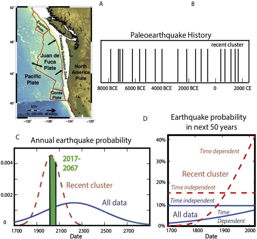
Rep. Prog. Phys. 84 (2021) 076801                                                                                                   Review

earthquakes is highly variable, and no observable precursors            However, this phenomenon has not been substantiated as a
should occur before them. If so, earthquake prediction is either        general phenomenon. Similar difficulties beset reports of a
impossible or nearly so.                                                decrease in the electrical resistivity of the ground before
    Support for this view comes from the failure to observe a           some earthquakes, consistent with large-scale microcracking.
compelling pattern of precursory behavior before earthquakes            Changes in the amount and composition of groundwater have
(Geller 1997). Various possible precursors have been sug-               also been observed. For example, a geyser in Calistoga, Cal-
gested—and some may have been real in certain cases—but                 ifornia, changed its period between eruptions before the M w
none have yet proved to be a general feature preceding all              6.9 1989 Loma Prieta and M w 5.7 1975 Oroville, California,
earthquakes, or to stand out convincingly from the normal               earthquakes.
range of the Earth’s variable behavior. In many previous cases,             Efforts have also been made to identify ground deforma-
it was not realized that a successful prediction scheme must            tion immediately preceding earthquakes. The most famous of
allow not only for successful predictions, but also failures-           these studies was the report in 1975 of 30–45 cm of uplift
to-predict and false alarms. Although it is tempting to note a          along the San Andreas fault near Palmdale, California. This
precursory pattern after an earthquake based on a small set of          highly publicized ‘Palmdale Bulge’ was interpreted as evi-
data and to suggest that the earthquake might have been pre-            dence of an impending large earthquake and was a factor in the
dicted, rigorous tests with large sets of data are needed to tell       US government’s decision to launch the National Earthquake
whether a possible precursory behavior is real, and whether             Hazards Reduction Program aimed at studying and predict-
it correlates with earthquakes more frequently than expected            ing earthquakes. US Geological Survey director Vincent McK-
purely by chance. In addition, after-the-fact searches for pre-         elvey expressed his view that ‘a great earthquake’ would occur
cursors have the advantage that one knows where to look. Most           ‘in the area presently affected by the. . . “Palmdale Bulge”. . .
crucially, any such pattern needs to be tested by predicting            possibly within the next decade’ that might cause up to 12 000
future earthquakes. That is why the RELM test of earthquake             deaths, 48 000 serious injuries, 40 000 damaged buildings,
forecasts (discussed below) was a significant advance.                  and up to $25 billion in damage. The California Seismic
    One class of precursors involves foreshocks, which are              Safety Commission stated that ‘the uplift should be consid-
smaller earthquakes that occur before a main shock, actually a          ered a possible threat to public safety’ and urged immediate
semantic definition. Many earthquakes, in hindsight, have fol-          action to prepare for a possible disaster. News media joined
lowed periods of anomalous seismicity. In some cases, there is          the cry.
a flurry of microseismicity, which are very small earthquakes               In the end, the earthquake did not occur, and reanalysis of
similar to the cracking that precedes the snap of a bent stick.         the data implied that the bulge had been an artifact of errors
In other cases, there is no preceding seismicity of any signif-         involved in referring the vertical motions to sea level via a tra-
icance. However, faults often show periods of either elevated           verse across the San Gabriel mountains. It was realized that
(‘activation’) or nonexistent (‘quiescent’) microseismicity that        the apparent bulging of the ground was produced by a com-
are not followed by a large earthquake. Alternatively, the level        bination of three systematic measurement errors. They were
of microseismicity before a large event can be unremarkable,            necessarily systematic in space and in time. The culprits were
occurring at a normal low level. The lack of a pattern highlights       (i) atmospheric refraction errors that made hills look too small,
the problem with possible earthquake precursors. To date, no            steadily declining as sight lengths were reduced from one lev-
changes that might be associated with an upcoming earthquake            eling survey to the next, which made the hills appear to rise, (ii)
are consistently distinguishable from the normal variations in          the misinterpretation of subsidence due to water withdrawal.
seismicity that are not followed by a large earthquake.                 Saugus was subsiding, as opposed to the areas surrounding
    Another class of possible precursors involves changes in the        Saugus uplifting! (iii) The inclusion of a bad rod in some of the
properties of rock within a fault zone preceding a large earth-         leveling surveys. These discoveries were led by (i) Bill Strange
quake. It has been suggested that as a region experiences a             of the NGS, (ii) Robert Reilinger (then at Cornell) and (iii)
buildup of elastic stress and strain, microcracks may form and          David Jackson at UCLA (Rundle and McNutt 1981, M Bevis,
fill with water, lowering the strength of the rock and eventually       personal communication, 2020).
leading to an earthquake. This effect has been advocated based              Hence the Bulge changed to ‘the Palmdale
on data showing changes in the level of radon gas, presumably           soufflé—flattened almost entirely by careful analysis of
reflecting the development of microcracks that allow radon to           data’ (Hough 2007). Subsequent studies elsewhere, using
escape. For example, the radon detected in groundwater rose             newer and more accurate techniques including the global
steadily in the months before the moment magnitude M w 6.9,             positioning system (GPS) satellites, satellite radar interfer-
1995 Kobe earthquake, increased further two weeks before the            ometry, and borehole strainmeters have not yet convincingly
earthquake, and then returned to a background level.                    detected precursory ground deformation.
    A variety of similar observations have been reported. In                An often-reported precursor that is even harder to quan-
some cases, the ratio of P- and S-wave speeds in the region             tify is anomalous animal behavior. What the animals are sens-
of an earthquake has been reported to have decreased by as              ing (high-frequency noise, electromagnetic fields, gas emis-
much as 10% before an earthquake. Such observations would               sions) is unclear. Moreover, because it is hard to distinguish
be consistent with laboratory experiments and would reflect             ‘anomalous’ behaviors from the usual range of animal behav-
cracks opening in the rock (lowering wave speeds) due to                iors, most such observations have been ‘postdictions,’ coming
increasing stress and later filling (increasing wave speeds).           after rather than before an earthquake.

                                                                    3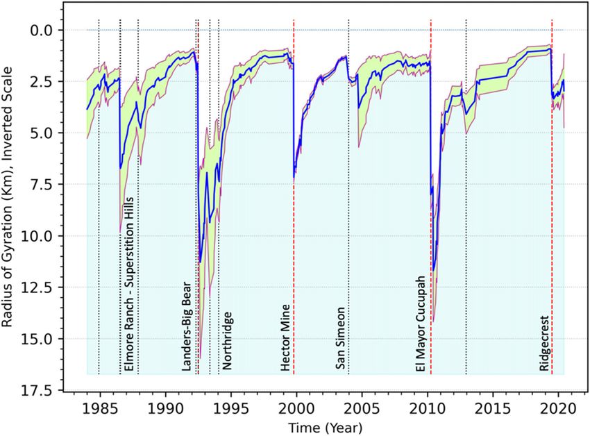
Rep. Prog. Phys. 84 (2021) 076801                                                                                                   Review

   Chinese scientists have attempted to predict earthquakes              1993). A likely explanation was that the uncertainty in the
using precursors. Chinese sources report a successful predic-            repeat time had been underestimated by discounting the fact
tion in which the city of Haicheng was evacuated in 1975, prior          that the 1934 earthquake did not fit the pattern well (figure 1)
to a magnitude 7.4 earthquake that damaged more than 90%                 (Savage 1993).
of the houses. The prediction is said to have been based on                 An earthquake eventually occurred near Parkfield on
precursors, including ground deformation, changes in the elec-           September 28, 2004, eleven years after the end of the predic-
tromagnetic field and groundwater levels, anomalous animal               tion window, with no detectable precursors that could have led
behavior, and significant foreshocks. However, in the follow-            to a short-term prediction (Kerr 2004). It is unclear whether
ing year, the magnitude 7.8 Tangshan earthquake occurred not             the 2004 event should be regarded as the predicted earthquake
too far away without precursors. In minutes, 250 000 people              coming too late, or just the next earthquake on that part of the
died, and another 500 000 people were injured. In the follow-            fault.
ing month, an earthquake warning in the Kwangtung province                  For that matter, we do not know whether the fact that earth-
caused people to sleep in tents for two months, but no earth-            quakes occurred about 22 years apart reflects an important
quake occurred. Similarly, no anomalous behavior was identi-             aspect of the physics of this particular part of the San Andreas,
fied before the magnitude 7.9 Wenchuan earthquake in 2008.               or just an apparent pattern that arose by chance given that we
Because foreign scientists have not yet been able to assess the          have a short history and many segments of the San Andreas
Chinese data and the record of predictions, including both false         of similar length. After all, flipping a coin enough times will
positives (predictions without earthquakes) and false negatives          give some impressive-looking patterns of heads or tails. With
(earthquakes without predictions), it is difficult to evaluate the       only a short set of data, we could easily interpret significance
program.                                                                 to what was actually a random fluctuation and thus be ‘fooled
   Despite tantalizing suggestions, at present there is still an         by randomness’ (e.g., Taleb 2004). It is possible the 1983 M w
absence of reliable precursors. Most researchers thus feel that          6.4 Coalinga earthquake (Kanamori 1983) was the ‘missing’
although earthquake prediction would be seismology’s great-              Parkfield event suggesting that earthquake forecasting should
est triumph, it is either far away or will never happen. How-            be based on regional spatial and temporal scales (Tiampo et al
ever, because success would be of enormous societal benefit,             2005) rather than fault based. As is usual with such questions,
the search for methods of earthquake prediction continues.               only time will tell.
To further this point, we now consider the famous Parkfield
earthquake prediction experiment.                                        2.1.2. Load unload response ratio (LURR). LURR is a
                                                                         method that was developed in China and is widely used by
                                                                         the Institute of Earthquake Forecasting of the China Earth-
2.1. The search for earthquake precursors
                                                                         quake Administration in the official yearly earthquake forecast
2.1.1. The Parkfield earthquake prediction experiment. Even              of China, which is required by law in that country (Yin et al
with the dates of previous major earthquakes, it is difficult            1995, 2004, Yuan et al 2010, Zhang et al 2008). However, this
to predict when the next one will occur, as illustrated by the           method has not been widely researched or used in other coun-
segment of the San Andreas fault near Parkfield, California,             tries. The basic idea is that tidal stresses on the Earth can be
a town of about 20 people whose motto is ‘be here when it                used as a diagnostic for the state of increasing stress prior to
happens.’ Earthquakes of magnitude 5–6 occurred in 1857,                 a major earthquake. Tidal stresses are cyclic, so in principle
1881, 1901, 1922, 1934, and 1966. The average recurrence                 there should exist an observable asymmetry in the response
interval is 22 years, and a linear fit to these dates made 1988          to the daily tidal stressing. Based on similar observations of
± 5 years the likely date of the next event. In 1985, it was             acoustic emissions from stressed rock samples in the labora-
predicted at the 95% confidence level that the next Parkfield            tory, it might be expected that microseismicity would be higher
earthquake would occur before 1993, which was the USA’s                  in the increasing stress part of the cycle, and lower in the de-
first official earthquake prediction (Bakun et al 2005).                 stressing part (Zhang et al 2008). However, data from actual
    Seismometers, strainmeters, creepmeters, GPS receivers,              field experiments are controversial (Smith and Sammis 2004).
tiltmeters, water level gauges, electromagnetic sensors, and
video cameras were set up to monitor what would hap-                     2.1.3. Accelerating moment release (AMR). AMR was a
pen before and during the earthquake. The US National                    method that was based on the hypothesis that, prior to frac-
Earthquake Prediction Evaluation Council endorsed the highly             tures in the laboratory and the field, there should be a pre-
publicized $20 million ‘Parkfield’ project. The Economist                cursory period of accelerating seismicity or slip, otherwise
magazine commented, ‘Parkfield is geophysics’ Waterloo. If               known as a ‘runup to failure’ (Varnes 1989, Bufe and Varnes
the earthquake comes without warnings of any kind, earth-                1993, Bufe et al 1994, Jaumé and Sykes 1999, Bowman and
quakes are unpredictable, and science is defeated. There will            King 2001, Sornette and Sammis 1995). In these papers, it
be no excuses left, for never has an ambush been more care-              was proposed that the accelerating slip is characterized by a
fully laid.’                                                             power law in time, therefore suggesting the possible existence
    Exactly that happened. The earthquake did not occur by               of critical point dynamics. While based on a reasonable physi-
1993, leading Science magazine to conclude, ‘seismologists’              cal hypothesis of a cascading sequence of material failure, the
first official earthquake forecast has failed, ushering in an era        phenomenology has so far not been observed in natural fault
of heightened uncertainty and more modest ambitions’ (Kerr               systems (Guilhem et al 2013).

                                                                     4
Rep. Prog. Phys. 84 (2021) 076801                                                                                                   Review

Figure 1. The Parkfield, CA earthquake that was predicted to occur within 5 years of 1988 did not occur until 2004. Black dots show when
the earthquake occurred, and the best-fitting line indicates when they should have occurred at intervals of 22 years.

3. Basic equations of earthquake science                                 where μ is the elastic modulus of rigidity, Δu is the average
                                                                         slip (discontinuity in displacement) across the fault, and A is
3.1. Observational laws                                                  the slipped area. Combining equations (1) and (2), we find that
                                                                         in fact, the GR law is a scaling relation (power law):
The oldest observational laws of earthquake science are the
Gutenberg–Richter (GR) magnitude-frequency relation and
                                                                                                N = 10a W {− 3 }
                                                                                                               2b

the Omori–Utsu relation for aftershock decay. The GR relation                                                                         (4)
states that the number of earthquakes M larger than a value m
                                                                         where m is given by (2).
in a given region and over a fixed time interval is given by:
                                                                            The remaining equation is the Omori–Utsu law (e.g.,
                      N (M  m) = 10a 10−bm .                  (1)       Scholz 2019), which was proposed by Omori following the
                                                                         1891 Nobi, Japan earthquake, surface wave magnitude M s
Here a and b are constants that depend on the time interval and          = 8.0, and expresses the temporal decay of the number of
the geographic region under consideration. Note further that             aftershocks following a main shock:
equation (1) is not a density function, rather it is a survivor
function or exceedance function.                                                                 dN      K
                                                                                                    =           .                     (5)
   The magnitude m was originally defined in terms of a local                                    dt   (c + t) p
magnitude developed by C F Richter, but the magnitude m is
                                                                         In (5), p, K and c are constants, to be found by fitting
now most commonly determined by the seismic moment W:
                                                                         equation (4) to the observational data, and t is the time elapsed
                       1.5m = log10 W − 9.0.                   (2)       since the main shock. In its original form, the constant c
                                                                         was not present, it was later added by Utsu to regularize the
Expression (2) is in SI notation. The quantity W is found from           equation at t = 0. An example of Omori–Utsu decay is shown
matching observational seismic timeseries obtained from seis-            in figure 3 below.
mometers to a model involving a pair of oriented and opposed
double-couples (dipoles), thus giving rise to a quadripolar              3.2. Elasticity
radiation pattern. Its scalar value is given by:
                                                                         Models to develop and test earthquake nowcast and forecast
                              W = μ Δu A                       (3)       methodologies are based on the known processes of brittle

                                                                     5
Rep. Prog. Phys. 84 (2021) 076801                                                                                                            Review

fracture in rocks, typically modeled as a shear fracture in an                    block. Then, for example, we can write the force or stress on
elastic material. The equations of linear elasticity are used to                  a slider block (=element of area) schematically as:
describe the physics of the process. Most of the models used
for nowcasting, forecasting and prediction are either statisti-                                        σi (t) =    Ti js j(t)              (12)
cal or elastostatic, where seismic radiation is neglected. The                                                     j

motivation for this approach is the focus on the slow processes
                                                                                  where the T i j are combinations of spring constants (discussed
leading up to the rupture, rather than on details of the rupture
                                                                                  below).
dynamics.
   To understand the basic methods, let us define a stress tensor
in d = 3:                                                                         4. Complexity and earthquake fault systems
                       σ(x, t) = σi j(x, t)                   (6)
                                                                                  Most researchers have now set their sights on probabilistic
and a strain tensor:                                                              earthquake forecasting, rather than deterministic earthquake

                                    1       ∂ui (x, t) ∂u j(x, t)                 prediction using precursors. The focus is presently on deter-
         ε(x, t) = εi j(x, t) =                       +                 (7)       mining whether forecasts covering months to years are feasi-
                                    2         ∂x j       ∂x i
                                                                                  ble, in addition perhaps to decadal time scales.
where the (infinitesimal) displacement in the elastic medium                         To understand the causes of the problems noted above, we
at location x and time t is u(x, t) = ui (x, t).                                  now briefly turn to an analysis of the structure and dynamics
    To relate the stress tensor to the strain tensor, the simplest                of earthquake faults systems, and how these may influence our
assumption is to use the constitutive law for isotropic linear                    ability to make reliable earthquake forecasts. We begin with
elasticity:                                                                       a discussion of the idea of earthquake cycles and supercycles.
                                                                                  In the context of complex systems, earthquake cycles can be
               σi j(x, t) = δi j λ εkk (x, t) + 2 μ εi j(x, t)          (8)
                                                                                  related to the idea of limit cycles in complex systems. In this
where δ ij is the Kronecker delta, μ and λ are the Lamé                          case a limit cycle is a repetitive behavior—a simple example
constants of linear elasticity, and repeated indices are summed.                  would be a sine wave. Of course, limit cycles are one man-
   The equation of elastic equilibrium can be stated in the                       ifestation of the dynamics of complex systems, others being
form:                                                                             chaotic and fixed-point dynamics.
                       ∇ · σ(x, t) = f (x, t)                (9)
                                                                                  4.1. Earthquake cycles and supercycles
where f(x, t) is a body force. It has been shown that the body
force appropriate to shear slip on a fault can be found by the                    Since the M w 7.9 San Francisco earthquake of April 18, 1906,
following method.                                                                 the dominant paradigm in earthquake seismology has been the
   For a fault element at position x , we wish to find the dis-                  earthquake cycle, in which strain accumulates between large
placement and stress at position x, i.e., we wish to find the                     earthquakes due to motion between the two sides of a locked
Green’s functions. To do so, we let:                                              fault. That strain is released by slip on the fault when an earth-
                                                                                quake occurs (Reid 1910). Over time, this process should con-
                  u x − x , t = û(t)δ(x − x )           (10)                   ceptually give rise to approximately periodic earthquakes and
                                                                                  a steady accumulation of cumulative displacement across the
where û is a unit vector, and δ(x) is the Dirac delta function.
                                                                                  fault.
We then compute the strain according to equation (7), followed
                                                                                      However, long records of large earthquakes using paleo-
by taking the divergence of that strain tensor. The result is
                                                                                  seismic records—geological data spanning thousands of years
solutions (Green’s functions) of the form:
                                                                                  or more—often show more complex behavior, as reviewed by

                                                                              Salditch et al (2020). The earthquakes occurred in supercycles,
          ui (x, t) = Gikl x − x Δuk x , t nl dA         (11)                   sequences of temporal clusters of seismicity, cumulative dis-

                                                                              placement, and cumulative strain release separated by intervals
         σi j (x, t) = Ti jkl x − x Δuk x , t nl dA.                            of lower levels of activity.

                                                                                     Supercycles pose a challenge for earthquake forecasting
    Here G     ikl x −
                        x is the displacement Green’s function,                  because such long-term variability is difficult to reconcile with
and T  i jkl x − x is the stress Green’s function. As before,                   commonly used models of earthquake recurrence (Stein and
Δuk x is the displacement discontinuity across the fault in                      Wysession 2009). In the Poisson model earthquakes occur ran-
kth direction at x , and nl is the unit normal to the fault, with                domly in time and the probability of a large earthquake is
dA being the element of fault area. Note that the detailed con-                   constant with time, so the fault has no memory of when the pre-
struction of these Green’s functions for point and rectangular                    vious large earthquake occurred. In a seismic cycle or renewal
faults can be found in many papers, with the most widely used                     model, the probability is quasi-periodic, dropping to zero after
version being found in the paper by Okada (1992).                                 a large earthquake, then increasing with time, so the probabil-
    In many of the simple models used to describe a single pla-                   ity of a large earthquake depends only on the time since the
nar fault, such as the slider block models discussed below, a                     past one, and the fault has only ‘short-term memory.’
spatial coarse graining is used to subdivide a fault into a par-                      This situation suggests that faults have ‘long-term
tition of squares of area ΔA, each square representing a slider                   memory,’ such that the occurrence of large earthquakes

                                                                              6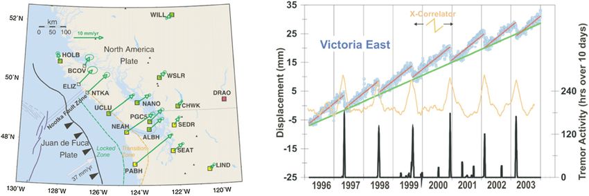
Rep. Prog. Phys. 84 (2021) 076801                                                                                                 Review

Figure 2. LTFM model. (Top) Simulated earthquake history. (Bottom) Earthquake probability versus time. Reprinted from (Salditch et al
2020), Copyright (2020), with permission from Elsevier.

depends on earthquake history over multiple previous                   strain, reflected in the probability P(t). The probability that an
earthquake cycles (figure 2). Faults having long-term mem-             earthquake occurs at time t, conditional on the history of strain
ory would have important consequences for earthquake                   accumulation and release at prior times, depends only on the
forecasting. Weldon et al (2004) point out that:                       most recent level of strain at time t − 1. Given P(t), the prob-
                                                                       ability does not otherwise depend on time, so the history prior
    ‘...resetting of the clock during each earthquake not
                                                                       to t is fully captured by P(t − 1).
   only is conceptually important but also forms the prac-
                                                                           LTFM can also be posed using the classic probability model
   tical basis for all earthquake forecasting because earth-
                                                                       of drawing balls from an urn (Stein and Stein 2013). If some
   quake recurrence is statistically modeled as a renewal
                                                                       balls are labeled ‘E’ for earthquake and others are labeled ‘N’
   process... In a renewal process, intervals between earth-
                                                                       for no earthquake, the probability of an earthquake is that of
   quakes must be unrelated so their variability can be
                                                                       drawing an E-ball, the ratio of the number of E-balls to the
   expressed by (and conditional probabilities calculated
                                                                       total number of balls. If after drawing a ball, we replace it, the
   from) independent random variables. Thus, if the next
                                                                       probability of an earthquake is constant or time-independent
   earthquake depends upon the strain history prior to that
                                                                       in successive draws, because one happening does not change
   earthquake cycle, both our understanding of Earth and
                                                                       the probability of another happening.
   our forecasts of earthquake hazard must be modified. . .
                                                                           Thus, an earthquake is never ‘overdue’ because one has not
   There can be little doubt that the simple renewal model
                                                                       happened recently, and the fact that one happened recently
   of an elastic rebound driven seismic cycle will need to be
                                                                       does not make another less likely. LTFM corresponds to an
   expanded to accommodate variations that span multiple               alternative sampling such that the fraction of E-balls and the
   seismic cycles.’                                                    probability of another event change with time. We add E-balls
    A simple model for supercycles, long-term fault mem-               after a draw when an earthquake does not occur and remove
ory (LTFM), extends the standard earthquake cycle model.               E-balls when one occurs. Thus, the probability of an earth-
It assumes that the probability of a large earthquake reflects         quake increases with time until one happens, after which it
the accumulated strain rather than elapsed time. The proba-            decreases and then grows again. Earthquakes are not inde-
bility increases as strain accumulates over time until an earth-       pendent, because one happening changes the probability of
quake happens, after which it decreases, but not necessarily to        another.
zero. Hence, the probability of an earthquake depends on the               Viewing supercycles as a result of LTFM fits into a gen-
earthquake history over multiple prior cycles.                         eral framework in the literature of complex dynamical systems.
    LTFM is a stochastic process, a Markov chain with states           Clustered events, described as ‘bursts,’ are observed in many
at discrete times corresponding to values of accumulated               disparate systems, from the firing system of a single neuron

                                                                   7
Rep. Prog. Phys. 84 (2021) 076801                                                                                                     Review

to an outgoing mobile phone sequence (Karsai et al 2012,                   laboratory settings in acoustic emission experiments, as well
Rundle and Donnellan 2020, discussed below). Such systems                  as in large scale field settings associated with tectonic faults
display ‘. . . a bursty, intermittent nature, characterized by short       (GR magnitude–frequency relation; Omori relation for after-
timeframes of intense activity followed by long times of no or             shocks). One important reason for this behavior is that driven
reduced activity,’ (Goh and Barabasi 2008). The system’s state             threshold systems of rock masses in which defects interact
depends on its history, so it has long-term memory (Beran et al            with long range interactions display near mean field dynam-
2013).                                                                     ics and ergodic behavior (Rundle and Klein 1989, Rundle et al
    LTFM simulations over timescales corresponding to the                  1996, Klein et al 1997, 2000a, 2000b, 2000c, 2007, Tiampo
duration of paleoseismic records find that the distribution                et al 2002a). This result, which was first proposed based on
of earthquake recurrence times can appear strongly periodic,               simulations and theory, was subsequently observed in field
weakly periodic, Poissonian, or bursty. Thus, a given paleo-               observations on the tectonic scale (Tiampo et al 2002b).
seismic window may not capture long-term trends in seismic-                    In both laboratory and field scale settings, a wide variety
ity. This effect is significant for earthquake hazard assessment           of timescales are also observed (Scholz 2019). These include
because whether an earthquake history is assumed to con-                   the source-process time scale of seconds to minutes on which
tain clusters can be more important than the probability den-              earthquakes occur, as well as the loading time scales of tens
sity function (pdf ) chosen to describe the recurrence times. In           to hundreds to thousands of years on which earthquakes recur
such cases, probability estimates of the next earthquake will              in active tectonic regions. Other phenomena, to be discussed
depend crucially on whether the cluster is treated as ongoing              below, such as small earthquake swarms and other thermal and
or finished.                                                               physical processes, operate on time scales as short as days, and
                                                                           as long as months to years (Scholz 2019).
4.2. Interactions and scales
                                                                               Modeling these types of processes requires consideration
Complex nonlinear systems are characterized by many inter-                 of fully interacting fields of dislocations, defects, damage, and
acting agents, each agent having some type of nonlinear behav-             other material disorder. In much of the previous work over the
ior, as well as interactions with other agents. They have a mul-           last decades on these types of systems, disordered fields were
tiplicity of scales in space and time, form coherent space–time            assumed to be non-interacting, allowing classical solid–solid
structures by means of their internal dynamics, have nonlinear             mixture theories to be employed (e.g., Hashin and Shtrickman
threshold dynamics, and are typically driven and dissipative               1962). With respect to earthquake faults, it was only empha-
(e.g., Rundle et al 2003). Examples of these types of systems              sized within the last few decades that earthquake faults interact
include markets and the economy, evolutionary, biological and              by means of transmission of tectonic stress, mediated by the
neural systems, the internet, flocking of birds and schooling of           presence of the brittle-elastic rocks within which the faults are
fish, earthquakes, and many more (Rundle et al 2019). None                 embedded.
of these systems evolve according to a central plan. Rather,                   With the development of new high-performance computing
their dynamics are guided by a few basic bottom-up principles              hardware and algorithms, together with new theoretical meth-
rather than a top-down organizational structure.                           ods based on statistical field theories, we can now model a wide
    In the example of earthquakes, these faults are embedded               variety of fully interacting disordered systems. One interesting
in complex geomaterials, and are driven by slowly accumu-                  example of such a macroscopic model is the interacting earth-
lating tectonic forces, or, in the case of induced seismicity,             quake fault system model ‘Virtual California’ (Rundle 1988,
by injection of fracking fluids. Rocks make up the Earth’s                 Heien and Sachs 2012), used in understanding the physics of
crust, and are disordered solids having a wide range of scales,            interacting earthquake fault systems. We will briefly consider
both structurally and dynamically as they deform (Turcotte and             and review this type of tectonic/macroscopic model in a later
Shcherbakov 2006, Turcotte et al 2003).                                    section, inasmuch as it allows the construction of simulation
    On the microscopic (micron) scale, dislocations and lat-               testbeds to carry out experiments on the dynamical timescales
tice defects within grains represent important contributors to             and spatial scales of interest.
solid deformation. On larger scales (millimeter), grain dynam-                 An interesting new development is associated with earth-
ics including shearing, microcrack formation, and changes                  quakes in regions where oil and gas are being mined, termed
in the porosity matrix contribute. On still larger scales (cen-            induced seismicity. These earthquake events are the result of
timeters to meters and larger), macroscopic fracturing in ten-             new fracking technology that has transformed previously rela-
sion and shear, asperity de-pinning, and other mechanical                  tively non-seismic regions—such as the US state of Oklahoma
processes lead to observable macroscopic deformation. On                   and the Groningen region of the Netherlands—into zones
the largest (tectonic) scales, the self-similarity is also man-            of frequent and damaging seismic activity (Luginbuhl et al
ifested as a wide array of earthquake faults on all scales,                2018c).
from the local to the tectonic plate scale of thousands of km                  In association with this new induced seismicity, an impor-
(Scholz 2019).                                                             tant new model that can be considered is the invasion percola-
    Observations of rock masses over this range of spatial scales          tion (‘IP’) model. IP was developed by Wilkinson and Willem-
indicate that the failure modes of these systems, such as frac-            sen (1983) and Wilkinson and Barsony (1984) at Schlum-
ture and other forms of catastrophic failure demonstrate scale             berger–Doll Research to describe the infiltration of a fluid-
invariant deformation, or power law behavior, characteristic               filled (‘oil’ or ‘gas’) porous rock by another invading fluid
of complex non-linear systems. These are observed in both                  (‘water’). The model has been studied by (Roux and Guyon

                                                                       8
Rep. Prog. Phys. 84 (2021) 076801                                                                                                      Review

1989, Knackstedt et al 2000, Ebrahimi 2010, Norris et al 2014,           (2γ). The bulk free energy tends to lower the overall energy
Rundle et al 2019) primarily for applications of extracting oil          at the expense of the surface free energy. In the case of ther-
and gas from reservoirs, and also in the context of the compu-           mal and magnetic phase transitions, the surface free energy is
tation of scaling exponents. Laboratory examples of IP have              also called a surface tension. Since the material damage that
also been observed (Roux and Wilkinson 1988).                            precedes fracture has a stochastic component, whether it is
    Until now, most of the research on this model has been               annealed or quenched, the relation between damage and failure
concerned with understanding the scaling exponents and uni-              is statistical. This makes the methods of statistical mechanics
versality class of the clusters produced by the model (Roux              relevant and the analysis of the relation between damage and
and Guyon 1989, Paczuski et al 1996, Knackstedt et al 2000).             catastrophic failure in simple models an important component
Direct application to flow in rocks has been discussed by                for elucidating general principles. Several excellent articles
Wettstein et al (2012).                                                  and texts in physics, materials science and Earth science com-
    Yet the physics of the model can be applied to a number of           munities document these ideas and serve as good references
other processes, for example the progressive development of              on progress in these fields (Alava et al 2006, Kelton and Greer
slip on a shear fracture or fault. Notable among the physical            2010, Ben-Zion 2008).
processes of IP is the concept of bursts. These can be defined               Earthquake seismicity has also been viewed as an example
as rapid changes in the configuration of the percolation lattice         of accumulating material damage leading to failure on a major
and correspond physically to the formation of a sub-lattice hav-         fault, and has been described by statistical field theories. For
ing greater permeability or conductivity than the site(s) from           example, one can decompose a strain field Ei j (x, t) into an
which the sub-lattice originates.                                        elastic εi j (x, t) and damage αi j(x, t) component:
    The multiplicity of these spatial and temporal scales,
together with the power-law scaling observed in the GR and                                Ei j (x, t) ≡ εi j (x, t) + αi j(x, t).        (15)
Omori statistical laws, lend support to the basic view that              One can then write a Ginzburg–Landau type field theory for
earthquake fault systems are examples of general complex                 the free energy for the energy in terms of the strain and dam-
dynamical systems, in many ways similar to systems seen                  age fields, and then find the Euler–Lagrange equation by a
elsewhere. Examples of other types of physical systems that              functional derivative. The result are equations that modify
display similar behaviors include stream networks, vascular              the elastic
networks, spin systems approaching criticality, and optimiza-                     moduli  in the constitutive laws by factors such as
                                                                         μ → μ 1 − α2 , so that as damage accumulates (α increases),
tion problems. Examples of systems from the social sciences              the rigidity of the material decreases, and large displacements
displaying similar dynamics include queuing problems, and                and fractures become inevitable.
social science network problems in biology and economics                    Earthquake nucleation has therefore been described as an
(Ebrahimi 2010).                                                         example of nucleation near a classical spinodal, or limit of
                                                                         stability (Klein et al 2000a, 2000b, 2000c). In this view, earth-
5. Nucleation and phase transitions                                      quake faults can enter a relatively long period of metastability,
                                                                         ending with an eventual slip event, an earthquake. Unlike clas-
5.1. Nucleation and fracture                                             sical nucleation, spinodal nucleation occurs when the range of
                                                                         interaction is long. In this physical picture, the slip on the fault,
The idea that earthquakes are a shear fracture has allowed
                                                                         or alternately the deficit in slip relative to the far-field plate
progress to be made using ideas from statistical physics. Frac-
                                                                         tectonic displacement, is the order parameter. Scaling of event
ture can be viewed as a catastrophic event that begins with
                                                                         sizes is observed in spinodal nucleation, but not in classical
nucleation, a first order phase transition. Griffith (1921) was
                                                                         nucleation.
the first to recognize that there is a similarity between nucle-
                                                                            Other views of earthquakes have emphasized the similarity
ation of droplets and/or bubbles in liquid and gases as pro-
                                                                         to second order phase transitions. Several authors view frac-
posed by Gibbs (1878), and fracture. For example, we note
                                                                         ture and earthquakes as a second order critical point (Sornette
that the Griffith (1921) model of an fracture or crack is found
                                                                         and Virieux 1992, Carlson and Langer 1989), rather than as a
by writing the free energy (Rundle and Klein 1989):
                                                                         nucleation event (Rundle and Klein 1989, Klein et al 1997).
                           F = −B l2 + 2γ l                  (13)        Recall that second order transitions, while they do show scal-
                                                                         ing of event sizes, are in fact equilibrium transitions, whereas
where B is a bulk free energy and 2γ is a surface free energy.           nucleation is a non-equilibrium transition. The heat generated
Or in other words, B is the elastic strain energy lost when a            by frictional sliding of the fault surfaces is considered to be the
crack of length l is introduced into the elastic material, and 2γ        analog of the latent heat in liquid–gas or magnetic first order
is the energy required to separate the crack surfaces. Instability       phase transitions.
occurs and the crack extends when the crack length l exceeds                Shekhawat et al (2013) used a two-dimensional model of a
a critical value lc determined by the extremum of F:                     fuse network to study the effect of system size on the nature
                                                                         and probability of a fracture event. A fuse network is a model
                         dF            γ
                            = 0 => lc = .                    (14)        in which an electric current is passed through an array of con-
                         dl            B                                 nected electrical fuses, which can burn out or fail if the current
   In general, nucleation is usually modeled as a competition            is too large. The model was used as an analog for fracture
between a bulk free energy (B), and a surface free energy                of materials. They argued that there were different regimes of

                                                                     9
Rep. Prog. Phys. 84 (2021) 076801 Review
fracture and established a phase diagram in which the nature of in the literature (Scholz 2019). Models for this type of pro-
the event crosses over from a fracture process that resembled cess are often characterized by the question of ‘why do earth-
a percolation transition (a second order transition) to one that quakes stop?’ A model for the cascade process was proposed
resembled the nucleation of a classical crack, as the system by Rundle et al (1998) based on the idea that slip events
size increased. Experimental support for the idea that fracture extend by means of a fractional Brownian walk through a ran-
is a phase transition can be seen in several investigations as dom field via a series of burst events. More recent work has
described below. related this type of Brownian walk to bond percolation theory
Laboratory experiments can elucidate the relation between (Rundle et al 2019).
material damage and the onset of a catastrophic failure event With respect to earthquakes as a kind of generalized phase
that could lead to material degradation. The latter, for example, transition and a cascade to failure, Varotsos et al (2001, 2002,
seems to be characteristic of the foreshocks that sometimes 2011, 2013, 2014, 2020) and Sarlis et al (2018) have proposed
seem to precede major earthquakes. Although there have been that earthquakes represent a dynamical phase transition asso-
significant advances in locating and characterizing this type ciated with an order parameter k1 . That parameter is defined
of precursory damage in materials (Li et al 2012, Hefferan as the variance of a time series of seismic electric signals
et al 2010, Guyer et al 1995, Guyer and Johnson 2009) there (SES). Furthermore, they define an entropy in natural time, and
has been little progress in relating the type and distribution of show that this quantity exhibits a series of critical fluctuations
damage to the onset of a major catastrophic failure such as is leading up to major earthquakes, both in simulation models,
observed in major earthquakes. and in nature (Varotsos et al 2011). These ideas depend on
Fracture under pressure in fiber boards has been studied by a definition of ‘natural time’, that is discussed in more detail
Garcimartin et al (1997) who recorded the acoustic emissions below (Varotsos et al 2001).
generated by the formation of micro cracks that preceded the Other work on similar ideas has been presented by Chen
catastrophic fracture event. Noting the power law size distribu- et al (2008a, 2008b). They proposed an alternative variant
tion of these events the authors conclude that the fracture could of the sandpile model with random internal connections to
be viewed as a critical phenomenon. Although there have been demonstrate the state of intermittent criticality or nucleation.
significant insights obtained from studies such as the ones cited The modified sandpile model (long-range connective sandpile
above, a general framework that can unify these results is still model) has characteristics of power-law frequency–size dis-
lacking and many questions remain. tribution. The model shows reductions in the scaling expo-
Damage can also initiate nucleation via the heterogeneous nents before large avalanches that mimics the possible reduc-
nucleation process. A great deal of work has been done to tion of GR b-values in real seismicity (Lee et al 2008). Lee
understand heterogeneous nucleation in special cases such as et al (2012) also consider failure in a fiber-bundle model to
nucleation on surfaces (Klein et al 1997, 2000a, 2000b, 2000c, address the problem of precursory damage. The study observes
2007, 2009, Kelton and Greer 2010, Muller et al 2000, Koster a clearly defined nucleation phase followed by a catastrophic
et al 1990) and aerosols (Flossman et al 1985, Hamill et al rupture (Lee et al 2012).
1977, Hegg and Baker 2009). As with fracture, an overall
framework is lacking. The role of defects such as vacancies
6. Earthquake data
or dislocations in crystal–crystal transitions is not understood
(Kelton and Greer 2010), and neither is the effect of quench
Earthquake data that are available for the study of dynamical
rates in multi-component systems (Gunton et al 1983).
processes fall into several categories. The first is seismicity
The fact that the state of the fields of nucleation and fracture
data, that includes hypocentral data from catalogs, which list
are similar is not surprising. They are in many ways the same
the location of initial slip, the magnitude of the eventual earth-
phenomenon. As noted, Griffith (1921) was the first to under-
quake, and the origin time. Other data are measures of sur-
stand that the formation of a classical crack in a brittle mate-
face deformation, including global navigation satellite system
rial was a nucleation event. Rundle and Klein (1989) adapted
(GNSS) data, previously referred to as GPS data. Another form
a field theoretic approach used to study nucleation near the
of surface deformation data arises from radar satellites or air-
spinodal in long range interaction systems (Unger and Klein
craft that illuminate the Earth and can be processed into inter-
1984). Their model was applied to nucleation in metals. They
ferometric synthetic aperture radar (InSAR) products. Stereo
obtained a theoretical description of the process zone asso-
photogrammetric pairs can also be used to determine deforma-
ciated with acoustic emissions produced by molecular bonds
tion from large events. These are the primary types of data that
breaking ahead of the advancing crack opening (e.g., Broberg
we discuss, although still other types of data include chemical,
1999).
thermal, and electromagnetic (Donnellan et al 2019).
5.2. Nucleation and failure cascades 6.1. Earthquake seismicity
The idea of spinodal nucleation as a process leading to earth- Earthquake data are organized and available in online cata-
quakes is associated with the idea that earthquakes are part logs maintained by organizations such as the USGS. Cata-
of a cascading process, where earthquakes that begin with log data include the origin time, magnitude, latitude, longi-
small slipping areas progressively overcoming ‘pinned’ sites tude, depth and other descriptive information on the location
to grow into large events. Pinned sites are called ‘asperities’ where the earthquake rupture first begins (the hypocenter).
10Rep. Prog. Phys. 84 (2021) 076801 Review
Figure 3. Seismicity having magnitudes M 2 within 600 km of Los Angeles from 1992–1995.
Magnitudes can be of several types, but the most used is the a number of vital earthquake-related parameters (e.g. Hudnut
moment magnitude scale, based on the seismic moment of et al 1994, Tsuji et al 1995).
the event (Hanks and Kanamori 1979). The seismic moment GNSS is also useful for tracking crustal deformation asso-
is a measure of the mechanical and thermal energy release ciated with the earthquake cycle (e.g. Hager et al 1991, Sagiya
of the system as the earthquake occurs and is typically com- et al 2000). GNSS data an also be used to illuminate many of
puted by fitting models of the source to waveforms observed on the processes present in postseismic deformation, and thereby
seismograms. to contribute understanding to earthquake physics (Melbourne
The data show that earthquakes of all magnitudes are known et al 2002). GNSS can even be used to track tsunami waves that
to cluster strongly in space and time (e.g., Scholz 2019, arise as a result of great submarine earthquakes for communi-
Reasenberg 1985). As noted, such burst phenomena are widely ties nearest the earthquake’s epicentre and as they propagate
observed in many areas of science (Bahar Halpern et al 2015, to distant coastlines around the world through the effects of
Mantegna and Stanley 2004, Paczuski et al 1996). One can ionospheric gravity waves (LaBrecque et al 2019). In short,
introduce a definition of seismic bursts that encompasses both GNSS measurement of crustal deformation can be used to
seismic swarms and aftershock sequences, with applications measure tectonic deformation prior to earthquakes, coseismic
to other types of clustered events as we describe below. An offsets from earthquakes with decreasing latency, and postseis-
example of aftershock sequences within 600 km of Los Ange- mic motions, all of which inform models of how the Earth’s
les in association with several major earthquakes is shown
crust accumulates strain, then fractures, and finally recovers.
in figure 3. It can be seen that the activity following the
Another important application of GNSS is the observation
main shock subsides to the background within several months.
and analysis of episodic tremor and slip (ETS), a phenomenon
This is an example of Omori’s law of aftershock occurrence
that was discovered by Dragert et al (Dragert et al 2001, 2004,
(e.g., Scholz 2019).
Brudzinski and Allen 2007) along the Cascadia subduction
zone along the Pacific Northwest coast of California, Ore-
6.2. Global navigation satellite systems (GNSS)
gon, Washington and British Columbia (figure 4). These events
GNSS data, of which GPS is one of the earliest and most famil- occur at relatively shallow depths of 30 km or so on the plate
iar examples, is another type of data being analyzed for use in interface and are associated with brief episodes of slip and
earthquake forecasting and nowcasting. Significant work has bursts of small earthquakes. ETS has been observed elsewhere
been done in the development of cost effective and efficient in the world as well, including such locations as Costa Rica
GNSS-based data systems to quickly and efficiently estimate (Walter et al 2011) and central Japan (Obara and Sekine 2009)
11Rep. Prog. Phys. 84 (2021) 076801 Review
Figure 4. Role of GNSS observations in the analysis of ETS. At left is the region of the Cascadia subduction zone off the Pacific Northwest,
showing a map of stations at which GNSS observations are routinely monitored. Of note are stations ALBH at the southern end of
Vancouver island, and station DRAO in the stable continental interior. At right above is shown the displacement of ALBH with respect to
DRAO over the years 1995–2004. Displacement is shown as the blue circles and red lines that represent best fits to the data. The green line
shows the steady aseismic trend. Bottom right is a record of the regional small earthquake bursts that accompany the slip events. The gold
line in the middle represents the correlation of the slip data with a detrended sawtooth curve, illustrating the repetitive nature of the events.
Reproduced from Dragert et al (2004). CC BY 4.0.
Measurement of crustal deformation to inform earthquake estimates of tsunami energy using GNSS for improved early
fault behavior dates back to the early 1980s (e.g., Davis et al warning (Titov et al 2016).
1989). By the early 1990s GNSS had been used to identify An important application of real-time GNSS data is for
additional contributions to the Pacific–North American plate tsunami early warning, as a result of great submarine earth-
motion from faults beyond the San Andreas fault proper (Feigl quakes. The 2004 M = 9.2 Sumatra–Andaman event (Ammon
et al 1993). On a more local to regional scale, GNSS crustal et al 2005, Ishii et al 2005, Lay et al 2005, Stein and Okal 2005,
deformation measurements combined with modeling identi- Subarya et al 2006) resulted in over 250 000 casualties, the
fied the geometry of faults near the Ventura basin and were majority of them on the nearby Sumatra mainland, with inun-
used to estimate the earthquake potential of the faults as capa- dation heights of up to 30 m (Paris et al 2007). Improvements
ble of producing an M6.4 earthquake (Donnellan et al 1993a, in earthquake forecasting can be expected to yield significant
1993b). In early 1994 the M = 6.7 Northridge earthquake benefits in tsunami warning as well. As another example, the
occurred (Jones et al 1994), demonstrating the value of apply- M = 8.8 2010 Maule earthquake in Chile (Lay et al 2010,
ing measurement of crustal deformation to earthquake hazard Delouis et al 2010) resulted in 124 tsunami related fatalities
assessment. and wave heights up to 15–30 m in the near-source coast (Fritz
The success of GNSS for understanding earthquakes led et al 2011).
to the deployment of continuous GNSS networks in Califor- Still another example is the 2011 M = 9.0 Tohoku-oki
nia (Blewitt et al 1993, Bock et al 1993, Hudnut et al 2001), earthquake in Japan (Simons et al 2011, Lay and Kanamori
the western US (Herring et al 2016), Japan (Tsukahara 1997), 2011), which generated a tsunami with inundation amplitudes
and globally (Larson et al 1997). By the early 2010s GPS net- as high as 40 m. That event resulted in over 15 000 casualties
works were relied on for understanding crustal deformation (Mori and Takahashi 2012) and was the first case of a large
and fault activity. Surface deformation was incorporated into tsunami impinging upon a heavily developed and industrial-
the most recent Uniform California Earthquake Rupture Fore- ized coastline in modern times. In addition to the tragic loss of
cast version 3 (UCERF-3) led by the USGS with input from the life, the economic collapse of the near-source coastline, which
California Geological Survey (CGS) and research community spans nearly 400 km, was almost complete (Hayashi 2012).
(Field et al 2013, Field et al 2014). These long-term forecasts Retrospective analysis in simulated real-time mode of high-
provide an assessment of earthquake hazard and intermediate rate (1 Hz) GNSS (primarily GPS) data was collected during
fault behavior. the 2011 Tohoku-oki event on the Japanese mainland from a
Retrospective real-time analysis of GNSS networks have network of more than 1000 stations. Those data convincingly
shown that the moments and slip displacement patterns of demonstrated that tsunami warnings in coastal regions imme-
large magnitude earthquakes can be calculated within 3–5 min diately adjacent to large events could be effectively issued
(Ruhl et al 2017, Melgar et al 2020). Furthermore, algorithms without regard for magnitude or faulting type (Melgar and
now exist to use these earthquake source models to assess the Bock 2013, Song et al 2012, Xu and Song 2013).
likelihood of tsunamis and to predict the extent, inundation By 2020, there will be over 160 GNSS satellites including
and runup of tsunami waves. Recently for example, a joint those of GPS, European Galileo, Russian GLONASS, Chinese
NOAA/NASA effort has further demonstrated the consistent BeiDou, Japanese QZSS, Indian IRNSS and other satellite
12You can also read