Reproducing size distributions of swarms of barchan dunes on Mars and Earth using a mean-field model
←
→
Page content transcription
If your browser does not render page correctly, please read the page content below

Reproducing size distributions of swarms of barchan dunes on
                                                           Mars and Earth using a mean-field model
arXiv:2110.15850v1 [physics.geo-ph] 29 Oct 2021

                                                                Dominic T Robson1 , Alessia Annibale2 , and Andreas CW Baas1
                                                   1
                                                       King’s College London, Department of Geography, Bush House, North East Wing, 40 Aldwych, London, UK,
                                                                                                    WC2B 4BG
                                                   2
                                                       King’s College London, Deparment of Mathematics, Strand Building, Strand Campus, Strand, London, UK,
                                                                                                     WC26 2LS

                                                                                                 October 2021

                                                                                                     Abstract
                                                              We apply a mean-field model of interactions between migrating barchan dunes, the CAFE
                                                          model, which includes calving, aggregation, fragmentation, and mass-exchange, yielding a
                                                          steady-state size distribution that can be resolved for different choices of interaction parame-
                                                          ters. The CAFE model is applied to empirically measured distributions of dune sizes in two
                                                          barchan swarms on Mars, three swarms in Morocco, and one in Mauritania, each containing
                                                          1000 bedforms, comparing the observed size distributions to the steady-states of the CAFE
                                                          model. We find that the distributions in the Martian swarm are very similar to the swarm
                                                          measured in Mauritania, suggesting that the two very different planetary environments how-
                                                          ever share similar dune interaction dynamics. Optimisation of the model parameters of three
                                                          specific configurations of the CAFE model shows that the fit of the theoretical steady-state
                                                          is often superior to the typically assumed log-normal. In all cases, the optimised parameters
                                                          indicate that mass-exchange is the most frequent type of interaction. Calving is found to occur
                                                          rarely in most of the swarms, with a highest rate of only 9% of events, showing that interactions
                                                          between multiple dunes rather than spontaneous calving are the driver of barchan size distri-
                                                          butions. Finally, the implementation of interaction parameters derived from 3D simulations of
                                                          dune-pair collisions indicates that sand flux between dunes is more important in producing the
                                                          size distributions of the Moroccan swarms than of those in Mauritania and on Mars.

                                                                                                         1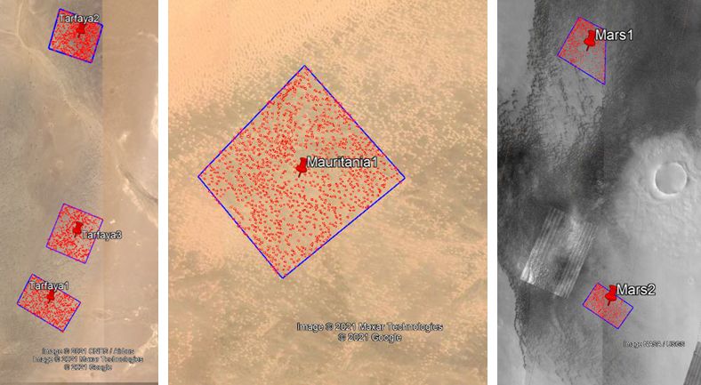
1    Introduction
Barchan dunes are a class of aeolian bedform that are found in many areas on Mars and Earth
under unidirectional wind regimes and relatively low sediment supply conditions [1, 2]. Under
such a near-constant wind direction, the dunes form into their striking crescentic shape with steep
slip-faces resulting from avalanching [3]. Properties of individual barchans, such as relationships
between migration rate and size or between the various morphometric parameters, are well-known
[3, 4, 5, 6, 7, 8, 9, 10, 11]. However, simulations have shown that the size of isolated barchans
is not stable but should rather grow indefinitely or shrink and vanish [12, 13, 14, 15, 16]. In re-
ality, barchans are not found as isolated dunes but in vast collections, known as swarms, which
can contain tens of thousands of dunes [14, 4, 17, 18]. By now it has been established that within
these swarms the size distribution of barchans is homogeneous in the direction of the wind. This
homogeneity contrasts with the instability observed in simulations where one would expect that
the average size should increase linearly with downwind distance [18]. The discrepancy between
simulated and observed behaviours suggests that the apparent stability of barchans in swarms is
an emergent property resulting from the interactions of the dunes. There are two main types of
interaction that are thought to be important in barchan swarms: calving, where a large dune breaks
into two smaller ones [4, 19, 20], and collisions [17, 18, 21, 22, 23].

    Owing to the long timescales over which these processes occur in real-world dune fields, stud-
ies of these interactions are typically performed using computer simulations [17, 12, 22, 24] or in
water-tanks in laboratories [21, 25, 26]. However, it is not clear that the results of simulations
and water-tanks experiments are entirely scalable to the real world. In this work, we explore an
alternative approach whereby the steady-state distribution of a mean-field model is fit to the size
distributions of real-world barchan swarms by adjusting the rules for the different interactions.
Mean-field models have previously been used to study barchan swarms [17, 23], however, these
models did not feature adjustable collision rules and did not include all of the types of interaction
known to occur in these systems.

    We recently developed a generalised mean-field model which can be applied to understand
the steady-state distributions of collections interacting bodies [27]. The model unites continuous
aggregation-fragmentation and asset-exchange models and, as such, can include any n → m process
in which an extrinsic quantity is conserved. Despite the generality of the processes permitted in the
model, it is possible to analytically derive the integer moments of the steady-state distribution of
the conserved quantity as well as find a self-consistency equation for the steady-state distribution
itself. Although any processes can be included, for this work we limited ourselves to only those
processes which have been observed in experiments and simulations. We compared the steady-state
outputs of this modelling to real-world size distributions which we measured for several locations
on both Mars and Earth.

    In section 2 we provide a description of the mean-field model and tailor the results of the
generalised model [27] to the processes which are relevant to barchan swarms. We then describe, in
section 3, the methods by which we measured the sizes of the real-world barchans and the locations
of the swarms we studied. In section 4 we show the distributions we observed for the swarms,
describe how we then optimised the model parameters to reproduce these, and show the results of
the optimisation, reserving discussion of the physical relevance of these findings and how the work

                                                 2
may be improved to sections 5 and 6.

2     Mean-field modelling
Mean-field models are useful tools in studying the global properties of large populations. The model
we apply in this work is a specific implementation of the general mean-field model which we have
described in [27].

2.1    Interactions
We consider a system comprising N (t) interacting particles (dunes) at time t. The dunes are charac-
terised by their volume, a continuous quantity distributed according to a volume probability density
function (pdf) p(v, t). Note here that, since the bulk density will be approximately the same in all
the barchans within a field, volume is equivalent to mass.

   In the general model [27] we allowed for any n → m interactions in which volume is conserved.
Here we limit ourselves to only those interactions which are known to be relevant in barchan swarms,
focusing on four interactions:

    • Calving - a 1 → 2 process where a dune spontaneously breaks apart.
    • Aggregation - a 2 → 1 process where two dunes merge together.
    • Fragmentation - a 2 → 3 process where two dunes break into three.

    • Exchange - a 2 → 2 process where volume is transferred between the dunes.

    Calving is thought to occur in barchan swarms due to changes in the wind or events such as
storms which can destabilise larger dunes resulting in a smaller barchan breaking off of the flank
[4, 28]. Barchans have been observed to aggregate (typically termed merging) in real-world fields
[5] as well as in simulations [17, 12, 18] and water-tank experiments [21].

    Fragmentation interactions have also been observed in various settings [17, 12, 18, 21, 19]
with several different types of fragmentation (e.g. “fragmentation-chasing” and “fragmentation-
exchange” [21]) having been described. In our model, we include only one 2 → 3 process as it is not
clear if the different types of fragmentation interaction produce significantly different outputs. We
would also like to note that, in the barchan literature, “calving” sometimes also refers to a 2 → 3
process [4, 19] however in this work we will only use the term to describe the spontaneous 1 → 2
process.

   Finally, the exchange process has also been observed in nature [29], simulations [17, 12, 18, 30],
and experiments [21].

    Since the model we are describing in this work features only these four interactions we will refer
to it as the Calving, Aggregation, Fragmentation, and Exchange (CAFE) model.

                                                  3
For the CAFE model we assume that all four interactions conserve volume so that the total
volume of all the dunes in the system is conserved. In real-world systems, we believe that collisions
ought to be at least approximately conservative, and this assumption is in line with previous agent-
based and mean-field modelling of barchan fields [17, 18, 23, 20, 22, 31].

2.2    Output channels and interaction rules
In [27] we introduce the concept of output channels (OCs) which is pivotal in our derivations.
OCs give expressions, based on the choice of interaction rules, for the individual outputs of all
the possible types of interaction. There are two outputs of calving, one of aggregation, three of
fragmentation, and two of exchange so we have eight OCs in our model here.

    Consider a dune of volume va calving to yield dunes with volumes v1 and v2 these are OC1 and
OC2. Volume conservation tells us that v1 +v2 = va but we need one additional piece of information
to determine the two volumes. This additional piece of information is the interaction rule for the
calving process, in this case, the ratio between the two output dunes, rc (always taking the smaller
dune in the numerator). To derive analytical results in [27] we only consider random interactions.
We make the same choice again here defining our interaction rule as a probability distribution,
pc (rc ), which is the distribution from which the stochastic variable rc = v2 /v1 is drawn. We now
have enough information to define the two OCs associated with calving
                                            va                     va rc
                                   v1 =            and v2 =              .                            (1)
                                          1 + rc                  1 + rc
For the remainder of the interactions we consider inputs va and vb and introducing additional
stochastic variables rf1 , rf2 , and re drawn from distributions pf1 (rf1 ), pf2 (rf2 ), and pe (re ). The
OCs are then defined as for aggregation,

                                               v3 = va + vb ,                                         (2)
for fragmentation,
                                             va + vb
                                        v4 =         ,                                                (3)
                                             1 + rf1
                                                (va + vb )rf1
                                        v5 =                      ,                                   (4)
                                             (1 + rf1 )(1 + rf2 )
                                              (va + vb )rf1 rf2
                                        v6 =                      ,                                   (5)
                                             (1 + rf1 )(1 + rf2 )

and for exchange collisions

                                                 v a + vb
                                            v7 =          ,                                           (6)
                                                  1 + re
                                                 (va + vb )re
                                            v8 =              .                                       (7)
                                                     1 + re

                                                     4
2.3     Rates and channel probabilities
Evaluating the time evolution of p(v, t) requires understanding how often the OCs create a dune of
volume v. We have already defined the OCs but have yet to discuss the rate at which the interac-
tions occur.

    Since we are considering a mean-field model, in any n-body interaction,       all combinations of
n-dunes must be equally likely to be involved. At time t there are Nn(t) such combinations and


therefore the rate at which n-body interactions occur is proportional to Nn(t) . We refer to the


proportionality constants as rate coefficients which we label αc , αa , αf , and αe for calving, aggre-
gation, fragmentation, and exchange respectively. OC1 and OC2 are outputs of calving, a one-body
interaction, while the other OCs are results of two-body interactions. We can now write the channel
probabilities pi which are given as the rate of a particular channel divided by the total rates of all
channels αout [27]

                                            αc
                               p1 = p2 =        N (t),                                             (8)
                                           αout
                                      αa
                               p3 =       N (t)(N (t) − 1),                                        (9)
                                    2αout
                                                 αf
                               p4 = p5 = p6 =         N (t)(N (t) − 1),                           (10)
                                               2αout
                                           αe
                               p7 = p8 =        N (t)(N (t) − 1),                                 (11)
                                         2αout
where
                                            αa + 3αf + 2αe
                         αout = 2αc N (t) +                  N (t)(N (t) − 1).                   (12)
                                                    2
Channel probabilities represent the fractions of dunes in the population that were generated through
each OC, while αout gives the total rate at which outputs are generated. Together with the defini-
tions of the output channels, we have now completely defined the CAFE model. The key aspects
of the model are shown pictorially in figure 1.

    The free parameters of the model are the rate coefficients, the distributions of the stochastic
variables, and the total volume of all the dunes. If we know the steady-state population size,
Ns , not all of the rate coefficients are free parameters since the steady population size requires a
balance between the additive interactions (fragmentation and calving) and the reductive interactions
(aggregation). In the CAFE model, the steady-state population size is
                                                         2αc
                                         Ns = 1 +              ,                                  (13)
                                                       αa − αf
which we use as a constraint on αa .

2.4     Master equation and steady-state probability density function
Having completely defined the model we can now insert all of the terms into the general equations
we derived in [27]. The evolution of p(v, t) is determined by the balance between the creation of

                                                   5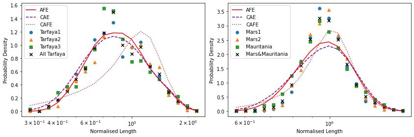
Figure 1: The four processes (left to right: calving, aggregation, fragmentation, and exchange),
eight output channels of the CAFE model (v1,...,8 ), and the definitions of the stochastic variables
(rc , rf1 , rf2 , and re ) which define the interaction rules. The rate coefficients αc , αa , αf , αe of the
four processes are also shown.

dunes of volume v through the output channels, and the loss of dunes of volume v due to such dunes
being involved in interactions. The balance of the loss and gain terms combine to give a master
equation for the time-derivative of p(v, t)
                                                  αout
                                     ṗ(v, t) =         pgain (v, t) − p(v, t) ,                                     (14)
                                                  N (t)
where

                    pgain (v, t) = δ vi (va , vb , rc , rf1 , rf2 , re ) − v        i,va ,vb ,rc ,rf1 ,rf2 ,re
                                                                                                                 ,   (15)

with δ(x) denoting the Dirac δ-function and h·ix the average over the distribution of x. Averaging
over the OCs is done using the channel probabilities, pi . Note that pgain (v, t) involves averaging
over the distributions of va and vb which are the volume pdf p(v, t) if we assume that the population
is large enough such that their distributions can be thought of as independent.

    It is trivial to write an expression for the steady-state volume pdf ps (v) by setting ṗ(v, t) = 0
in equation (14) which gives
                                                                               (s)
                       ps (v) = δ vi (va , vb , rc , rf1 , rf2 , re ) − v       i,va ,vb ,rc ,rf1 ,rf2 ,re
                                                                                                           ,         (16)

where we have used the superscript (s) to denote that the distributions of va and vb on the right
hand side of (16) are also the steady-state distribution ps (v). This is a self-consistency equation
as the steady-state pdf appears on both sides. The form of the self-consistency equation means,
however, that it can easily be solved using a population dynamics algorithm [27, 32, 33].

2.5     Steady-state moments
As well as a self-consistency equation for the steady-state pdf, it is also possible to write exact
expressions for the steady-state moments [27]. As we have already stated, the total volume of

                                                           6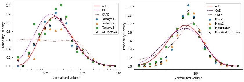
dunes in the system is a free parameter, which, when divided by the steady-state population size
Ns , gives the mean volume hvis , where the subscript, s, denotes that this is in the steady-state.
The higher integer moments hv ` is for ` ≥ 2 can then be calculated iteratively [27] using
`−1
` K` X `
hv is = hv j is hv `−j is , (17)
Z` j=1 j
where
1+r `
1 + rf`1 (1+rff2)`
* +
re`
Ns (Ns − 1) 2
1+
K` = αa + αf + αe (18)
(s) (1 + rf1 )` (1 + re )`
2αout rf1 ,rf2 re
and where
1 + rc`
αe Ns
Z` = 1 − 2K` − . (19)
(s)
αout (1 + rc )` rc
3 Measuring size distributions of real-world barchan swarms
In this section, we describe the locations of the real-world barchan swarms which we have measured
and the method we used for extracting the sizes of the dunes.
3.1 Zones of study
A swarm of barchan dunes is a two-dimensional many-body system in which the bedforms all mi-
grate in approximately the same direction, that of the dominant wind. Typically, mean-field models
such as ours do not apply to such low-dimensional systems because they rely upon an assumption
that the systems are well-mixed [34]. However, large swarms of barchans are thought to be homo-
geneous in the direction of the wind [4, 18]. As such, one can effectively treat a zone within the
bulk of a large swarm as having periodic boundaries, so that the assumption of sufficient mixing
is valid within the zone. Support for this claim can be found in [23] where size distributions in an
agent-based model with periodic boundaries were approximately replicated using mean-field models.
Although barchan swarms occur at many locations on Earth [2] and Mars [1], in most of these
locations the populations of barchans are limited in number and typically situated between different
classes of bedforms such as barchanoid ridges, meaning that the assumption of periodic boundaries
may not hold.
We limit ourselves to swarms in which we could define zones of ∼ 1000 barchans such that the
dunes immediately upwind of the zone appeared qualitatively similar to those within the zone. For
this study, we selected six zones: three located approximately 17km west of El Hagounia, Tarfaya
Province in a large field which extends southward from the northern Atlantic coast of Morocco; one
around 60km south of Akjoujt, Mauritania in a field that extends southwest towards the coast; and
two oriented east-southeast in the northern circumpolar region of Mars. The locations of these six
7Figure 2: The locations of the zones of study on Earth and on Mars are marked as stars. On Earth,
the more northerly star covers the locations of the three zones in Tarfaya Province while the more
southerly marker covers the field in Mauritania. Image courtesy of Google Earth.
zones are shown in figure 2.
Each zone contained at least 1000 bedforms, however not all of the bedforms within the zones
were barchan dunes but included also complex dunes, which were likely the intermediate stages
of collisions, and bedforms for which no slip-face was visible, these may have been proto-dunes or
dome dunes. Aerial images of the six zones are shown in figure 3.
3.2 Measuring dunes
We recorded seven locations on and around each dune body: the toe, the leftmost edge, the tip
of the left horn, the base of the slip-face, the brink, the tip of the right horn, and the rightmost
edge. These points are shown in figure 4. From these points, it is possible to determine any of the
morphological dimensions of the barchan.
Due to the high density of barchans in the zones of study, many of the barchans were not isolated
bedforms but were in the process of colliding. In these cases, it was not always possible to identify
all seven points on the dunes in which case we attempted to estimate their locations as shown in
figure 5. Such an attempt was made in all cases where there were two (or more) distinct crescents
in the slip-face. In cases where the leeward slope of a complex bedform exhibited some deformity
but only one crescent was visible in the slip-face, the bedform was regarded as a single barchan. In
some cases, the bedforms were deformed to such an extent that, although a slip-face was visible, it
was no longer crescentic. Such dunes were not recorded as barchans and so no attempt was made
to estimate the seven points; instead, we traced around the outline of the dune.
In addition to complex bedforms resulting from dune-dune interactions, some bedforms did not
have a visible slip-face. When no slip-face was visible, but the shape was otherwise distinctly that
of a barchan, it was assumed that the cause was poor image resolution and an attempt was made
8Figure 3: The size zones of study are marked as blue quadrilaterals with the bedforms inside
marked in red. The locations of the markers are: Tarfaya1 22◦ 220 1000 N 12◦ 340 1600 W, Tarfaya2
27◦ 280 5500 N 12◦ 330 2500 W, Tarfaya 3 27◦ 230 5000 N 12◦ 330 3100 W, Mauritania1 19◦ 120 2000 N 14◦ 230 3700 W,
Mars1 75◦ 10 000 N 72◦ 80 000 W, and Mars2 73◦ 460 000 N 70◦ 380 3700 W. Images courtesy of Google Earth.
9Figure 4: The seven points that were recorded on each barchan within the zones of study. Image
courtesy of Google Earth. The dominant wind direction is from the from the top of the image to
the bottom.
10to estimate the location of all seven points. Where there was no visible slip-face and the shape
of the bedform did not appear barchan-like we recorded only four points: the upwind, downwind,
leftmost, and rightmost extents of the bedform.
3.3 Determining volumes
From the seven points recorded on each of the barchans, we can calculate any linear dimension of
the dunes including horn-to-horn width, total width, windward length, and total length. However,
to compare the outputs of the mean-field model to the observations of the real-world fields, it was
necessary to calculate the volume of the bedforms from the linear dimensions. Previous studies
have shown how the volume of barchans scales as the cubic power of their height, length, and width
[4, 35, 36, 16, 12].
We found that the most reliable linear dimension was the length l, the distance between points
1 and 4 shown in figure 4. The length was the easiest dimension to extract since it did not require
correction for the orientation of the dune (as was necessary for determining the width). We also
found that there was a greater degree of subjectivity in locating exactly the position of the widest
point, while sand streaming off of the horns sometimes made defining the tip of the horn difficult.
On the other hand, we found that, in most cases, the toe and slip-face were easily identified, making
the length measurement more reliable than other dimensions. To calculate the volume v we used
the relation v = l3 /20 which is a good description of the barchans in the Tarfaya Province [4].
4 Results
We will now describe the observed size distributions, the method by which we optimised model
parameters, and the quality of the fits obtained using these optimal configurations. Discussion of
the physical relevance of the results will be left for the following section.
4.1 Observed size distributions
As we have mentioned, each of the zones of study contained over 1000 bedforms, however not all of
these bedforms were barchan dunes. Since the length-volume relation [4] only holds for barchans,
for this work we ignored all other bedforms and worked solely with the barchan size-distributions.
The population sizes in Tarafya zones 1, 2, and 3 were 927, 1112, and 850 respectively. The Mau-
ritanian zone contained 984 barchans while Mars 1 and 2 contained 977 and 975 respectively.
4.1.1 Length distributions
In the four terrestrial swarms, the average length of barchans was approximately equal; Tarfaya
zones 2 and 3 and the Mauritanian zone all had an average length of 23m while the barchans in
Tarfaya 1 were slightly larger with an average of 26m. We observed that the Martian barchans were
significantly larger than those on Earth with average lengths of 131m and 113m in Mars zones 1
and 2 respectively. The large discrepancy between dune sizes on Earth and Mars is likely caused by
differences in the mechanics of saltation in the two environments [37] but the sizes will also depend
11Figure 5: Example of mid-collision barchans where the locations of some of the seven points had
to be estimated. Image courtesy of Google Earth
12on sediment availability and other factors.
Although understanding these differences is important for understanding dune fields, the aver-
age size of dunes in a location is likely controlled by external environmental factors. In this work,
we are more interested in understanding how the internal processes of barchan-barchan interactions
govern the distribution about this mean. Therefore, for the remainder of this work, we will always
normalise lengths (and volumes) by the mean size of barchans in that zone allowing us to compare
the results from each of the different areas of study.
Figure 6 shows distributions of normalised length in each of the zones of study. The distri-
butions in the three Tarfaya zones are very similar which is unsurprising since these three zones
constitute different areas within a single large population of dunes. The similarity in these three
distributions and the similarity in average size in the Tarfaya zones suggests that our assumption
of homogeneity in large fields is valid and is in agreement with previous findings [4, 18]. A similar
argument could also be made for the two Martian fields, however, it is surprising that the Mauri-
tania zone has a very similar distribution to the fields on Mars despite the large difference in the
average size. The striking similarity between the Mauritanian and Martian data suggests that the
internal processes in the two locales are similar despite the environmental conditions being very dif-
ferent. These findings also potentially suggest that there may be a certain degree of universality of
size distributions, with different classes of barchan fields (e.g. Tarfaya-type, Mars-Mauritania-type).
Although the distributions in the Tarfaya zones are rather different to those in Mauritania and
Mars, all of the distributions can be well-approximated by log-normal distributions as has been
widely reported in previous studies [4, 17, 18]. This can also be seen in figure 6 where we show
log-normal distributions estimated using the method of moments.
4.1.2 Volume distributions
Since we have assumed that the volume of barchan is directly proportional to the cube of its length,
a log-normal distribution of lengths would correspond to a log-normal distribution of volumes.
However, the slight discrepancies between the observed length and the estimated log-normal dis-
tributions are exaggerated when converted to volume distributions. This is particularly obvious in
the Tarfaya data, where differences between the distributions close to the peak are particularly em-
phasised when converted to volumes as shown in figure 7. Note here that it is possible to optimise
the parameters of the log-normal distributions to produce a better fit to the data, however, our
objective was not to produce arbitrarily accurate empirical fits but rather to investigate how these
distributions could be produced solely through the interactions of the dunes.
4.2 Free parameters and optimisation procedure
As described in section 2.3, interactions in the CAFE model are governed by: the distributions of the
stochastic variables rc , rf1 , rf2 , and re ; and the rate coefficients αc , αa , αf , and αe . In all cases, αa
and αf are not independent and therefore we have only three free rate coefficients. This constraint
on a rate coefficient is the only constraint that exists in the CAFE model in general. However, it is
not possible to perform a generalised optimisation of the model since infinitely many free parameters
would be required to describe all of the possible distributions for the stochastic variables. To perform
13Figure 6: Probability density functions are shown for the lengths of barchans in each of the six zones
of study normalised by the average length in that zone. The lines show log-normal distributions
estimated from the mean and variance of the observed data.
14Figure 7: Observed probability density functions of barchan volumes calculated as v = l3 /20 in
the zones of study. The lines show log-normal distributions estimated from the moments of the
combined distributions of all three Tarfaya zones (solid line) and the Martian and Mauritanian
zones (dashed line).
15Model αc αa αf αe
AFE αc = 0 αa = (1 − αe )/2 αf = (1 − αe )/2 Free
CAE Free αa = 2αc /(N − 1) αf = 0 Free
CAFE Free αa = 2αc /(N − 1) + αf Free Free
Table 1: The rate coefficients in the uniform AFE, uniform CAE, and empirical CAFE models.
Where an equality is shown the parameter is constrained to take that value.
the optimisation, we, therefore, restrict ourselves to three specific implementations of the CAFE
model:
• The uniform AFE model where: αc = 0, αa = αf = (1 − αe )/2, and the stochastic variables
rf1 , rf2 , and re are each distributed uniformly in the ranges [rf1min , rf1max ], [rf2min , rf2max ],
and [remin , remax ] respectively.
• The uniform CAE model where: αc 6= 0, αf = 0, and αa = 2αc /(N − 1). The stochastic
variables rc and re are distributed uniformly in the ranges [rcmin , rcmax ] and [remin , remax ]
respectively.
• The empirical CAFE model where: αc 6= 0, αa = 2αc /(N − 1) + αf , the distributions of rf1
and re are determined from a known collision rule, and the distributions of rc and rf2 are
uniformly distributed in [rcmin , rcmax ] and [rf2min , rf2max ] respectively.
The uniform AFE and empirical CAFE model have 7 free parameters while the CAE model has
6. These are shown, together with the constraints in tables 1 and 2.
The dimensionality of the parameter spaces in these three model versions is low enough that the
optimisation algorithm (described in section 4.2.2) converged, for different initial conditions, in a
reasonable amount of time to a single minimum in each zone. Despite the reduction in parameters,
our choice of these three implementations allows for a wide investigation of the power of the general
CAFE model. The uniform AFE and CAE models sacrifice one of the types of interaction but allow
us to maintain the adjustability of the rules for the remaining processes. Comparison of these two
models allows us to comment upon how changing from calving to collisional fragmentation affects
the size distribution. Note also that we use uniform distributions for the stochastic variables as, in
this case, each of the terms appearing in equation (18) has an exact form.
The empirical CAFE model sacrifices some of the adjustability of the other models but includes
all of the processes. The distributions of re and rf1 are derived from a rule thought to be applicable
to real-world barchan collisions [17, 12, 18] and therefore the empirical CAFE model ought to be
realistic. However, none of the model implementations includes long-range interactions of barchans
in a swarm via exchange of sand flux. This means that the empirical CAFE model may not be able
to accurately reproduce distribution in swarms where sand flux plays a dominant role. On the other
hand, in the uniform AFE and CAE, the interaction rules can adjust themselves to compensate for
the lack of sand flux, and therefore may be able to give a better fit.
16Model pc (rc ) pf1 (rf1 ) pf2 (rf2 ) pe (re )
AFE n/a [rf1min , rf1max ] [rf2min , rf2max ] [remin , remax ]
CAE [rcmin , rcmax ] n/a n/a [remin , remax ]
CAFE [rcmin , rcmax ] Empirical [rf2min , rf2max ] Empirical
Table 2: The distributions of the four stochastic variables in the uniform AFE, uniform CAE, and
empirical CAFE models. We have used the shorthand [x, y] to denote a uniform distribution in the
range [x, y]. In all such cases, x and y are free model parameters. The empirical distributions were
derived from a known collision rule.
4.2.1 Empirical collision rule
In the empirical CAFE model we fix the distributions pf1 (rf1 ) and pe (re ) to a distribution we
derived using an empirical collision rule [17, 18]. The collision rule was developed by empirically
fitting the volume ratio of outputs of barchan-barchan collisions to a function of their lateral offset
and initial volume ratio [17, 12]. The details of the rule can be found in the appendix of [18]. The
collision rule has previously been used in mean-field modelling for exchange collisions only [17],
however, we also took the ratio rf1 to be given by the same rule since many fragmentation collisions
are similar to an exchange collision where one of the outputs subsequently breaks apart.
The empirical collision rule is deterministic given the initial volume ratio and lateral offset [18].
To implement this rule in the CAFE model we had to convert the deterministic expression into a
probability distribution of outputs. The method for doing this was:
1. Randomly select two dunes from our steady-state population and calculate their volume ratio
rin .
2. Generate a random value for the lateral offset θ from a uniform distribution in the range [0, 1].
3. Insert rin and θ into the deterministic collision rule [18] to give the output volume ratio rout .
4. Record rout and repeat until 106 values have been generated.
When running the empirical CAFE model, each time we were required to generate a random
value for re or rf1 we simply randomly selected one of these 106 deterministically calculated routs .
The resulting distributions for our datasets are shown in the left part of figure 8.
Before we proceeded with implementing this method using our real-world data, we first ensured
that the outputs generated from our stochastic distribution were the same as those generated when
using the deterministic rule itself. An example of this is shown in the right part of figure 8
4.2.2 Optimisation
Since we can solve for the steady-state distribution for a particular configuration of the CAFE
model, one method of optimising the parameters would have been to use some measure of similarity
between distributions, such as the Kolmogorov-Smirnov (KS) test statistic. as a cost function of
an optimisation routine. However, the time taken to solve for the steady-state, and the high
dimensionality of the parameter space, mean we would only be able to explore a small area of
17Figure 8: Left: The distributions used for re and rf1 in the empirical CAFE model for Tarfaya
datasets (solid line) and the Mars and Mauritania datasets (dashed line). Right: A comparison of
the steady-state distribution produced using the deterministic collision rule [18] and the stochastic
collision rule we derived from the deterministic one.
the space using this technique. Instead, we chose to make use of the fact that we have analytical
expressions for all of the integer moments (equation (17)). The computational time taken to solve
for the moments of the steady-state is therefore much less than solving for the entire steady-state.
We, therefore, defined a cost function as the average percentage difference between the first 9 non-
trivial moments of the observed and theoretical normalised volume distributions (since the volumes
are normalised, the first moment is unity) i.e.
s
10
1 X (E[v ` ] − hv ` is )2
λ= , (20)
9 E[v ` ]2
`=2
where E[v ] are the observed moments and hv ` is are the theoretical steady-state moments for a
`
given set of parameters calculated using equation (17). This cost function minimises the average
percentage error of the moments which, since the moments are rapidly increasing, means that the
cost function prefers models where the lower moments are close to the data and puts less constraint
on the higher moments. This is important since the lower moments are more stable to the pres-
ence of large outliers. We also found that implementing the generalised method of moments using
weightings calculated from a heteroskedasticity-consistent covariance matrix did not converge to an
optimum configuration within the permitted range of parameters (e.g. remin ∈ [0, 1] etc.)
The optimisation of the model then consisted of finding the global minimum of our cost function.
We performed this minimisation using the SciPy [38] implementation of dual annealing, a technique
which couples generalised annealing with a local search [39, 40, 41, 42, 43].
The generalised annealing searched through ∼ 3 × 10⁵ configurations of the parameters. When
the local search was included this increased to ∼ 106 parameter configurations. We ran the opti-
misation algorithm for each of the three models and for:
• Each of the three Tarfaya zones separately.
18• The combined distribution of all three Tarfaya zones.
• Both of the Mars zones and the Mauritania zone separately.
• The combined distribution of both Mars zones and the Mauritania zone.
Altogether this meant that 24 runs of the dual annealing were performed, in all of which the
algorithm converged to a minimum. We chose to group distributions in the way described above
to give larger data sets. We feel that this is also reasonable since the distributions appeared very
similar as shown in figures 6 and 7, suggesting the internal interactions were very similar.
4.3 Optimum parameters
We ran the population dynamics algorithm to find the steady-state distribution corresponding to
the optimum parameters we had found. We found that a small number of very large outliers in Mars
zone 1 and the Mauritania zone were significantly changing the observed moments in those fields
which led to the optimum parameters producing steady-states which were significantly different to
the observed distributions. Removing these outliers (five in Mars zone 1 and two in the Mauritania
zone) resulted in the optimum parameters producing steady-state distributions that were much
closer to the observation.
We show optimum parameters configurations for all of the observed distributions in table 3 for
the uniform AFE, uniform CAE, and empirical CAFE models respectively. To help with comparison
between the rate coefficients for calving and the collision process, we define event probabilities ρi
with i = c, a, f, or e
αc N
ρc = , (21)
αc N + (αa + αf + αe )N (N − 1)/2
αa,f,e N (N − 1)
ρa,f,e = . (22)
2αc N + (αa + αf + αe )N (N − 1)
These event probabilities, ρc,a,f,e , are the probabilities the next event (calving or collision) to occur
in the system will be calving, aggregation, fragmentation, or exchange accounting for the different
dependence of the rate coefficients on population size. Note also that since these four events are
the only processes in our model ρc + ρa + ρf + ρe = 1. In the case of the uniform AFE model
ρa = ρf = (1 − ρe )/2 since the rates of fragmentation and aggregation must balance in order for
a steady-state to exist. Similarly, in the uniform CAE model ρa = ρc and in the empirical CAFE
model ρa = ρc + ρf .
Across the three different models, we observe certain similarities in the optimised parameters.
First and foremost we see that ρe > 0.50 in all cases and ρe > 0.8 in most instances. This means
that exchange collisions make up the majority of interactions regardless of the model chosen which
is in agreement with simulations of barchan-barchan collisions where exchange interactions are ob-
served to result from the greatest range of input parameters [17].
Fragmentation and aggregation were found to be uncommon when using the uniform AFE with
the most frequent occurrence found for the combined Tarfaya dataset where ρa = ρf = 5.5%.
19Likewise, in the uniform CAE model the relative probabilities of calving and aggregation collisions
were ρc = ρa < 2.5%. The highest optimised rates of non-exchange interactions were found using
the empirical CAFE model which found probabilities ρa ≈ ρf = 0.23 for Tarfaya 3. The optimised
empirical CAFE parameters for Mars 1 were ρc ≈ ρa = 9.2% which was the highest value for the
probability of calving observed in any of the fields.
In the Tarfaya zones, the uniform AFE and uniform CAE converged to the same result, where
exchange collisions were considerably more frequent than the other types of interactions, and the
average volume ratio of the outputs of an exchange collision was in the range [0.2, 0.3] (i.e. on
average one output was between 3.3 and 5 times larger than the other). It is also worth noting
that the optimum model parameters relating to the distributions of rf1 and rf2 (in the uniform
AFE model) were found to be very similar in all of the zones with rf1min = 1.0, rf1max = 2.8, and
rf2min = rf2max = 1.0 found to be the optimum in all but one case. These distributions of rf1 and
rf2 mean that the outputs of fragmentation collision are two equally sized small dunes and then
a larger dune with a volume between 2 and 5.6 times as large as each of the small dunes. Frag-
mentation of this type, where the result is one large dune and two similarly sized smaller dunes,
has been seen in both water tanks experiments and simulations of barchan collisions (e.g. centred
“fragmentation-chasing” in [21] and “budding” in[44]). In contrast, for the empirical CAFE model,
rf2 was found to only take very small values, i.e. one of the two smaller dunes is much larger than
the other, this is more similar to the “neighbouring effect” described in [19].
The calving parameters were found to be less consistent for the different zones than the frag-
mentation rules. In the uniform CAE the size of the smaller dune was always in the range 44-100%
of the size of the larger output of calving however the exact values varied significantly between the
zones. This type of calving is very different to how the process is understood in the real world,
where rc ought to be a lot smaller since only large dunes calve and the new dune is created at the
minimum size [28, 19]. The rule for calving in the empirical CAFE model is much more in line with
that conception of the process.
Finally, it may seem surprising at first that the optimal parameters for the combined distribution
of several zones may differ significantly from those found for the zones individually. For instance,
one can see in table 3 that ρe = 1.0 in each of the Tarfaya zones individually however, when
combined, the optimum value obtained was ρe = 0.89. This can be explained by looking at the
optimum parameters of the stochastic variables in these instances. We can see that in each of the
individual zones remin ≈ remax in which case (bearing in mind ρe = 1.0 for the individual zones)
the theoretical moments are
1 + ri`
hv ` ii = , (23)
(1 + ri )`
(i) (i)
where we use i = 1, 2, 3 to represent Tarfaya 1, 2, and 3 respectively and ri = remin = remax . The
combined distribution has moments
3
X Ni hV ` ii
hv ` itot = , (24)
i=1
Ntot
where Ni is the population size of that zone and Ntot = N1 + N2 + N3 is the total population size
20of all three zones. Owing to the non-linearity of equation (23), the total moments cannot generally
be re-written in the same form i.e. there does not, in general, exist an r for which
1 + r`
hv ` itot = . (25)
(1 + r)`
Hence, the optimum parameter configuration for the combined dataset does not look the same as
any of the individual zones. Similar arguments can be applied to the other discrepancies between
the combined datasets and their constituents in the other models.
21Model&Zone ρc ρa ρf ρe rcmin rcmax rf1min rf1max rf2min rf2max remin remax
AFE T1 n/a neg. neg. 1.0 n/a n/a n/c n/c n/c n/c 0.27 0.27
AFE T2 n/a neg. neg. 1.0 n/a n/a n/c n/c n/c n/c 0.29 0.29
AFE T3 n/a neg. neg. 1.0 n/a n/a n/c n/c n/c n/c 0.20 0.20
AFE TALL n/a 0.054 0.054 0.89 n/a n/a 1.0 2.8 1.0 1.0 0.23 0.25
AFE M1 n/a 0.014 0.014 0.97 n/a n/a 1.0 2.8 1.0 1.0 0.27 0.98
AFE M2 n/a 0.043 0.043 0.91 n/a n/a 1.0 2.8 1.0 1.0 0.31 1.0
AFE Mau. n/a 0.016 0.016 0.97 n/a n/a 1.0 2.8 1.0 1.0 0.21 1.0
AFE MMau. n/a 0.027 0.027 0.95 n/a n/a 0.98 4.22 0.89 1.0 0.26 0.99
CAE T1 neg. neg. n/a 1.0 n/c n/c n/a n/a n/a n/a 0.27 0.27
CAE T2 neg. neg. n/a 1.0 n/c n/c n/a n/a n/a n/a 0.29 0.29
CAE T3 neg. neg. n/a 1.0 n/c n/c n/a n/a n/a n/a 0.20 0.20
CAE TAll 0.012 0.012 n/a 0.98 0.82 0.86 n/a n/a n/a n/a 0.10 0.40
CAE M1 2.2 × 10⁻³ 2.2 × 10⁻³ n/a 1.0 1.0 1.0 n/a n/a n/a n/a 0.23 1.0
CAE M2 0.023 0.023 n/a 0.95 0.57 0.69 n/a n/a n/a n/a 0.25 1.0
22
CAE Mau. 3.8 × 10⁻³ 3.8 × 10⁻³ n/a 0.99 0.70 0.93 n/a n/a n/a n/a 0.18 1.0
CAE MMau. 0.013 0.013 n/a 0.97 0.67 0.75 n/a n/a n/a n/a 0.22 1.0
CAFE T1 2.8 × 10⁻³ 0.10 0.10 0.79 0.047 0.075 n/a n/a 8.9 × 10⁻⁴ 2.9 × 10⁻³ n/a n/a
CAFE T2 2.1 × 10⁻³ 0.082 0.080 0.84 4.6 × 10⁻³ 0.19 n/a n/a 7.1 × 10⁻⁴ 1.9 × 10⁻³ n/a n/a
CAFE T3 9.1 × 10⁻⁴ 0.23 0.23 0.53 0.083 0.11 n/a n/a 1.1 × 10⁻³ 1.5 × 10⁻³ n/a n/a
CAFE TAll neg. 0.18 0.18 0.63 0.21 0.25 n/a n/a 3.3 × 10⁻⁶ 6.3 × 10⁻⁶ n/a n/a
CAFE M1 0.091 0.092 7.3 × 10⁻⁴ 0.82 0.93 0.94 n/a n/a 0.11 0.66 n/a n/a
CAFE M2 neg. neg. neg. 1.0 n/c n/c n/a n/a n/c n/c n/a n/a
CAFE Mau. 9.6 × 10⁻³ 9.6 × 10⁻³ neg. 0.98 0.94 0.99 n/a n/a n/c n/c n/a n/a
CAFE MMau. neg. neg. neg. 1.0 n/c n/c n/a n/a n/c n/c n/a n/a
Table 3: The optimum parameters for the uniform AFE, uniform CAE, and empirical CAFE models for all datasets which were: the three
Tarfaya zones (T1, T2, T3), the combined Tarfaya dataset (TAll), the two Martian zones (M1, M2), the Mauritania zone (Mau.), and the
combined Mars+Mauritania dataset (MMau.). Event probabilities ρc,a,f,e marked “neg.” had optimum values smaller than O(10−5 ) or
smaller. Values marked “n/a” were not applicable to that model while entries marked “n/c” were not constrained since the relevant event
probability was negligible.Figure 9: The normalised steady-state volume distributions corresponding to the optimised parame-
ters for the uniform AFE, uniform CAE, and empirical CAFE models for: the combined distribution
of all three Tarfaya zones (left) and the combined distributions of the two Martian zones and the
Mauritanian zone (right) with the data from the fields themselves shown as points.
4.4 Steady-state distributions
The parameters were inserted into a population dynamics algorithm [27, 32, 33] to find their corre-
sponding steady-state distributions. In figure 9 we show the volume distributions of steady-states
for the optimised parameters calculated for: the combined distribution of the three Tarfaya zones
and the combined distribution of the Martian and Mauritanian zones. One can see that reasonable
fits are achieved in both cases for the uniform AFE and uniform CAE models while the empirical
CAFE model gives a very poor fit to the Tarfaya data. Since the raw data we obtained was the
lengths of the dunes we also show the steady-state length distributions in figure 10
To quantitatively evaluate the strength of each fit we calculated two-sample KS statistics from
the raw datasets and the steady-state outputs of the three models. The KS statistics for the three
models and a log-normal estimated from the first two moments are shown in table 4. From these KS
statistics, we can see that the uniform AFE and uniform CAE can produce steady-state distributions
which fit the data more accurately than a log-normal in the case of the Tarfaya datasets while the
empirical collision rule CAFE model yields a much poorer fit (though still comparable to the log-
normal). In the case of the Martian and Mauritanian data, we see that the uniform AFE and
empirical CAFE generally give similar fits to the data while the uniform CAE model gives a worse
fit. For the Martian and Mauritanian data, the estimated log-normal gives a better fit than any of
the models.
5 Discussion of results
The fact that the Martian and Mauritanian datasets appear to fit one another very closely is sur-
prising. Given the large differences between the environments of Mars and Mauritania their close
fit strongly suggests that it is indeed the internal processes of dune interactions that govern the
shape of the size distributions, with external controls determining the average size.
23Figure 10: The steady-state distributions of normalised length corresponding to the optimised
parameters for the uniform AFE, uniform CAE, and empirical CAFE models for: the combined
distribution of all three Tarfaya zones (left) and the combined distributions of the two Martian
zones and the Mauritanian zone (right), with the data from the fields themselves shown as points.
AFE CAE CAFE log-normal
Tarfaya1 0.051 0.050 0.13 0.11
Tarfaya2 0.033 0.033 0.13 0.10
Tarfaya3 0.073 0.077 0.15 0.11
Tarfaya1&2 0.037 0.041 0.12 0.11
All Tarfaya 0.026 0.044 0.12 0.10
Mars1 0.086 0.10 0.16 0.084
Mars2 0.077 0.11 0.079 0.036
Both Mars 0.083 0.11 0.078 0.038
Mauritania 0.072 0.089 0.076 0.041
Mars and Mauritania 0.078 0.10 0.063 0.037
Table 4: Two-sample Kolmogorov-Smirnov (KS) statistics calculated between the observed distri-
butions and the optimised model steady-states for the three models and all of the different datasets.
For reference we have also included KS statistics for log-normal distributions with parameters es-
timated from the first two moments.
24Our choice to fit combined datasets as well as individual zones led to the important finding that
the optimum interaction rules for combined distributions could be very different to those in each
of their constituent parts. Although this seems counterintuitive, we have already argued why this
is the case in the AFE model, and similar arguments can be applied in the other models. This
finding suggests that the most important role played by calving, fragmentation, and aggregation is
to generate slight variations between the local distributions in different parts of a swarm. Qualita-
tively the distributions in the three Tarfaya zones seem to be roughly the same and so homogeneity
appears to hold fairly well for the swarm as a whole. However, the subtle differences between these
zones mean that the global distribution cannot be accurately reproduced without the inclusion of
non-exchange processes. Swarms in which calving, aggregation, or fragmentation are prevalent are
likely, therefore, to exhibit greater zonal differences in size distribution.
Comparing the fits (table 4) of the uniform AFE and uniform CAE models to the data, we see
that, except in the cases where the two had converged to the same result, the AFE model gives a
better fit to the data than does the CAE model. This result implies that fragmentation, especially
where the two smaller outputs are similarly sized, is more likely than calving to play the role of
driving regional variations as described above. However, in the empirical CAFE model, fragmen-
tation collisions are preferred for the Tarfaya datasets while calving is preferred for the Mars and
Mauritania data. Our results are therefore inconclusive as to whether calving or fragmentation is
more important in barchan swarms although, in either case, exchange collisions are the dominant
interaction.
In the case of the Martian and Mauritanian data, we saw that the fits produced by the empirical
CAFE model were much better than in the case of the Tarfaya dunes. An important process in the
development of barchan swarms that we have omitted is that of sand flux between the dunes. In
previous mean-field modelling where the deterministic collision rule that we adapted was used, the
distributions produced using only exchange collisions were then deformed in such a way as to try
and mimic the role of sand flux [17]. In that work, the amount of deformation required to match the
collision-only steady-state distribution to the real-world distributions was used to infer how relevant
sand flux was compared to collisions in each field [17]. Using the same logic, we might therefore
conclude that, assuming the empirical collision rule is applicable in Mauritania and on Mars, sand
flux plays much less of a role in those settings than in Tarfaya. However, in a later work using the
same deterministic collision rule as in [17] it was found that exchange collisions alone could not
negate the coarsening effect whereby average dune size increases with downwind distance due to
sand flux [18]. The authors of that work concluded that fragmentation processes must therefore be
involved to counteract this, however, we found that the optimum rates of calving (spontaneous frag-
mentation) and collisional fragmentation were small in the Martian and Mauritanian fields (see ρc
and ρf in table 3) and therefore it is unlikely that they would be able to undermine this coarsening
effect. It, therefore, remains an open question as to how homogeneity might arise in barchan fields
despite sand flux, given that both the simulations of collisions [17] and our work suggest that the
overall rate of fragmentation is low. A possible explanation of this is that large barchans undergo
calving at a much greater rate than smaller ones, or that there is some minimum size for calving
to occur [28, 20], which was not considered in our model.
Another point that can be made from our model is that, especially in the case of the Martian
25and Mauritanian dunes, the differences between the distribution produced using our three model
implementations are not very significant (see figure 10). Considering this, and the fact that other
authors have been able to produce similar distributions using different modelling [17], we can see
that it is likely that the size distribution of barchans alone is not enough to determine the nature
of interactions in swarms. This suggests one must consider other properties of the fields such as
the spatial structuring.
It is worth noting also that our results indicate that a log-normal is not necessarily an entirely
accurate description of the distribution of barchan sizes. In figure 6 we show log-normals that
quite closely replicate the observed length distributions. However, when we convert the lengths
to volumes, the differences between the log-normal and actual distributions are more pronounced
and it becomes less obvious that the log-normal distribution is an accurate description, especially
in the case of the Tarfaya data. Indeed, we are able to produce distributions using the uniform
AFE and uniform CAE models that provide a much closer fit to the Tarfaya distributions than
does a log-normal. The reported log-normal fit for a length (or other linear dimensions) distribu-
tion may therefore be, in part, due to the volume-length (or volume-width) scaling laws for barchans.
Finally, we have shown that it is possible to produce good fits to the size distributions we ob-
served for barchan swarms in nature using three different implementations of the CAFE model.
In previous modelling, [17] many characteristics of these distributions have also been reproduced
in models where interactions are treated very differently. This implies that there is not enough
information contained in global size distributions in barchan swarms to precisely constrain the in-
teraction rules. For this reason, while it is theoretically possible to extend the CAFE model to
include sand flux and a different treatment of calving, we do not feel that these additional factors
would lead to greater insight. However, the fact that our finding that exchange collisions are domi-
nant agrees with continuum simulations [17, 12] suggests that, although global size distributions are
not sufficient to precisely determine the interaction rules, there is enough information to provide
some constraint. This type of modelling remains very useful, therefore, in understanding the role of
interactions in shaping barchan size distributions. Rather than proceeding to add to the complexity
of a mean-field model, extensions to this work should focus on adding additional information in the
form of spatial structuring in barchan swarms and extending the model to be spatially explicit e.g.
an agent-based model rather than a mean-field one.
6 Conclusion
We applied a mean-field particle-collision model representing calving, aggregation, fragmentation,
and exchange (CAFE) interactions between migrating dunes in barchan swarms to replicate their
measured size distributions on Mars and Earth, with three sample areas near Tarfaya, Morocco,
one in Mauritania, and two in the Mars’ northern circumpolar region.
Fitted model parameters reveal the relative importance of the interaction types and the poten-
tial role played by sand flux.
Two distinct classes of distributions were observed: 1) Mars and Mauritania exhibit strikingly
similar size distributions, suggesting that the interactions are comparable despite the different plan-
etary environments; 2) the three Tarfaya sample areas show similar size distributions and model
26results imply that sand flux is more important in these swarms. The optimised model steady-state
solutions give reasonable fits to the size distributions in the swarms, in several cases providing a
better fit than the expected log-normal distribution. The results show that exchange is the domi-
nant interaction type for all swarms making up at least 53%, and more typically > 80%, of events.
Fragmentation and aggregation are much less prevalent, making up at most 23% of events each,
and more often < 10%. Calving is found to represent . 1% of events in most instances, with the
highest rate found to be 9.1%. Generally, the fits produced by the models are better when the rate
of non-exchange interactions is low. The results suggest that collisions, especially exchange, play a
more important role than calving in shaping size distributions in barchan swarms. We furthermore
find that processes other than exchange are most important in swarms where there are local varia-
tions in the size distribution.
Including sand flux and adapting calving so that only larger barchans are able to calve are
possible extensions to the model. However, both would prevent the analytical calculation of the
moments. Additionally, we have been able to replicate the distributions using different implemen-
tations of a model and other authors have also been able to reproduce similar distributions using
other types of models. This suggests that there is not enough information contained within the
global size distribution alone. Nevertheless, the results we have presented provide some answers to
open questions on the roles of calving, collision, and sand flux in barchan swarms.
Acknowledgments
DTR is supported by the EPSRC Centre for Doctoral Training in Cross-Disciplinary Approaches
to Non-Equilibrium Systems (CANES EP/L015854/1).
27References
[1] Mary C Bourke and Andrew S Goudie. Varieties of barchan form in the namib desert and on
mars. Aeolian Research, 1(1-2):45–54, 2009.
[2] Andrew S Goudie. Global barchans: A distributional analysis. Aeolian Research, 44:100591,
2020.
[3] Ralph A Bagnold. The Physics of Blown Sand and Desert Dunes. Methuen, London, 1941.
[4] Hicham Elbelrhiti, Bruno Andreotti, and Philippe Claudin. Barchan dune corridors: field
characterization and investigation of control parameters. Journal of Geophysical Research:
Earth Surface, 113(F2), 2008.
[5] S Parker Gay Jr. Observations regarding the movement of barchan sand dunes in the nazca
to tanaca area of southern peru. Geomorphology, 27(3-4):279–293, 1999.
[6] El-Sayed Sedek Abu Seif and Mohamed H El-Khashab. Desertification risk assessment of sand
dunes in middle egypt: a geotechnical environmental study. Arabian Journal for Science and
Engineering, 44(1):357–375, 2019.
[7] MA Hamdan, AA Refaat, and M Abdel Wahed. Morphologic characteristics and migration
rate assessment of barchan dunes in the southeastern western desert of egypt. Geomorphology,
257:57–74, 2016.
[8] Ammar Amin and El-Sayed Sedek Abu Seif. Environmental hazards of sand dunes, south
jeddah, saudi arabia: an assessment and mitigation geotechnical study. Earth Systems and
Environment, 3(2):173–188, 2019.
[9] Bin Yang, Yong Su, Nan He, Bo Zhang, Xiaosi Zhou, and Yang Zhang. Experimental study
on the stable morphology and self-attraction effect of subaqueous barchan dunes. Advanced
Powder Technology, 31(3):1032–1039, 2020.
[10] Junhuai Yang, Zhibao Dong, Zhengyao Liu, Weikang Shi, Guoxiang Chen, Tianjie Shao, and
Hanmin Zeng. Migration of barchan dunes in the western quruq desert, northwestern china.
Earth Surface Processes and Landforms, 44(10):2016–2029, 2019.
[11] Fangen Hu, Xiaoping Yang, and Hongwei Li. Origin and morphology of barchan and linear
clay dunes in the shuhongtu basin, alashan plateau, china. Geomorphology, 339:114–126, 2019.
[12] Orencio Durán, Eric JR Parteli, and Hans J Herrmann. A continuous model for sand dunes:
Review, new developments and application to barchan dunes and barchan dune fields. Earth
Surface Processes and Landforms, 35(13):1591–1600, 2010.
[13] Bruno Andreotti, Philippe Claudin, and S Douady. Selection of dune shapes and velocities
part 2: A two-dimensional modelling. The European Physical Journal B-Condensed Matter
and Complex Systems, 28(3):341–352, 2002.
[14] Pascal Hersen, Ken Haste Andersen, Hicham Elbelrhiti, Bruno Andreotti, Philippe Claudin,
and Stéphane Douady. Corridors of barchan dunes: Stability and size selection. Physical
Review E, 69(1):011304, 2004.
28You can also read


