Rotation Period Detection for Earth-like Exoplanets - CalTech ...
←
→
Page content transcription
If your browser does not render page correctly, please read the page content below
Rotation Period Detection for Earth-like Exoplanets
Jiazheng Li1, Jonathan H. Jiang2, Huanzhou Yang3, Dorian S. Abbot3, Renyu Hu2, Thaddeus D.
Komacek3, Stuart J. Bartlett1 and Yuk L. Yung1, 2
1
  Division of Geological and Planetary Science, California Institute of Technology, Pasadena, CA, USA
2
  Jet Propulsion Laboratory, California Institute of Technology, Pasadena, CA, USA
3
  Department of the Geophysical Sciences, The University of Chicago, Chicago, IL, USA

Corresponding author: Jiazheng Li (jiazheng@caltech.edu)

Abstract
    A terrestrial planet’s rotation period is one of the key parameters that determines its climate
and habitability. Current methods for detecting the rotation period of exoplanets are not suitable
for terrestrial exoplanets. Here we demonstrate that, under certain conditions, the rotation period
of an Earth-like exoplanet will be detectable using direct-imaging techniques. We use a global
climate model to simulate reflected starlight from an Earth-like exoplanet and explore how
different parameters (e.g., observing direction, wavelength, time resolution) influence the
detectability of the planet’s rotation period. We show that the rotation period of an Earth-like
exoplanet is detectable using visible channels with time-series monitoring at a signal-to-noise
ratio >20 with ~5 – 15 rotation periods of data, while the rotation period of a planet with full ocean
coverage is unlikely to be detected. Our results provide useful guidance for rotation period
detection of Earth-like exoplanets using future space telescopes.

1. Introduction
    Since the rotation rate of a planet determines its Coriolis force, and therefore strongly
influences its atmospheric and oceanic circulation, it is one of the key parameters that determines
the climate of a planet (Showman et al., 2013; Forget and Leconte, 2014; Kaspi and Showman,
2015; Komacek and Abbot, 2019). Moreover, as a result of cloud feedbacks, simulations suggest
that a slowly rotating Earth-like planet could maintain a habitable climate at nearly twice stellar
flux as the Earth, which implies a strong dependence of the inner edge of the habitable zone on
planetary rotation rate (Yang et al., 2014; Way et al., 2016). Therefore, detecting the rotation
period of an exoplanet is crucial for evaluating its habitability. Furthermore, the rotation period of
an exoplanet will evolve towards the orbital period due to the tidal forces exerted by the star it
orbits, especially for potential habitable exoplanets orbiting low-mass stars (Kasting et al. 1993).

                                                                                                        1
Barnes (2017) calculated that about half of the habitable Kepler planets and most of the habitable
Transiting Exoplanet Survey Satellite (TESS) planets should be tidally locked within 1 Gyr.
Detecting the rotation period of an exoplanet, and determining whether it is tidally locked, will
therefore put constraints on the age of an exoplanetary system.
   A number of methods are currently being used to detect the rotation period of exoplanets. The
first method is to use the rotational broadening of the spectrum of a gas to determine the rotational
velocity of the exoplanet. For example, Snellen et al. (2014) used the CO spectrum to constrain
the rotation velocity of the gas giant β Pictoris b and Brogi et al. (2016) used the CO and H2O
spectra to constrain the rotational velocity of HD 189733b. The second method is to infer the
rotation period of an exoplanet from the magnetic-field-induced radio emission from the exosolar
system. For example, Hess and Zarka (2011) modeled the radio dynamic spectra from an exoplanet
and its parent star to show that physical information about the system, including the magnetic field
and the rotation period of the exoplanet, can be obtained from the radio observations.
       These two methods are optimal for hot Jupiters and directly imaged wide-separation gas
giant planets, which are likely to have high rotation rates, strong absorption of certain gases or
strong magnetic fields. As a result, these methods are not suitable for detecting the rotation period
of Earth-like exoplanets. In the foreseeable future, the best chance we are likely to have to detect
the rotation period of an Earth-like exoplanet is by analyzing the single-pixel observation of the
reflected starlight from the exoplanet, which can be used to retrieve the surface features (Fan et
al., 2019; Aizawa et al., 2020; Gu et al., 2021). Although the reflected starlight of an Earth-like
exoplanet will be extremely faint compare to its star, high-contrast imaging capabilities such as a
coronagraph or starshade (an external occulter in a telescope designed to suppress the light from
the star; Cash, 2006; Vanderbei et al., 2007) will allow us to directly image Earth-like exoplanets.
For example, in an overview of the noise budget of starshade-assisted exoplanet imaging, Hu et
al. (2021) showed that for some nearby stars (for example, tau Ceti and epsilon Indi A), a signal-
to-noise ratio of 20 in a narrow spectral band can be achieved for an Earth-size planet in the
habitable zone of its host star with an integration time of several hours using a HabEx-like
telescope. The integration time would be shorter for a wider bandpass. It should therefore be
feasible to detect the rotation period of Earth-like exoplanets in the future.
   In this study, we explore the detectability of the rotation period of an Earth-like exoplanet.. We
use the exoplanetary community atmospheric model (ExoCAM) global climate model (GCM) to

                                                                                                   2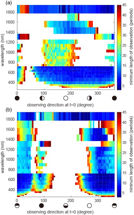
simulate the atmospheric dynamics and radiative transfer for an Earth-like exoplanet with different
rotation periods. Using the simulation results, we mimic future observations of an exoplanet and
study which parameters of the exoplanet determine the detectability of its rotation period. We also
explore the direction, wavelength, time duration, and frequency of simulated observations. We
describe ExoCAM in Section 2. In Section 3, we show how we mimic exoplanet observations and
obtain the rotation period from them. We investigate the influence of different parameters on the
detectability of rotation period in Section 4. We present a summary and discussion in Section 5.

2. ExoCAM GCM
   We use the ExoCAM GCM (Wolf & Toon 2015; Kopparapu et al. 2016, 2017; Wolf et al.
2017; Wolf 2017) to simulate the atmosphere of a range of exoplanets. ExoCAM is a global climate
model modified from the Community Atmosphere Model version 4 (CAM4). It uses correlated-k
radiative transfer with updated spectral coefficients using the HITRAN 2012 database and a novel
treatment of water vapor continuum absorption. Crucially for this project, ExoCAM provides
radiative output in XX wavelength bins. ExoCAM has previously been used for a wide variety of
studies of the atmospheric circulation and climate of terrestrial exoplanets, including cloud
behavior (Wolf & Toon 2015; Kopparapu et al. 2016, 2017; Wolf et al. 2017; Wolf 2017; Haqq-
Misra et al. 2018; Komacek & Abbot 2019; Yang et al. 2019, May et al. 2021).
   We conduct two GCM experiments which are equivalent except that they have different
rotation periods (one day and two days). Each simulation has an Earth-like ocean-land distribution,
planetary radius, surface gravity, obliquity (23.5°), orbital eccentricity (0.0167) and orbital period.
The atmosphere is purely composed of nitrogen gas, N2. The irradiation is the same as that on
Earth (1360 W/m2) and the incident stellar spectrum is the same as the Sun’s. The ocean is
simulated with a 50-meter-deep slab-ocean model with thermodynamic sea ice (Bitz et al. 2012).
We use a horizontal grid of 4°×5° with 40 horizontal layers (Komacek & Abbot 2019). The
experiments typically last for about 15 years with a time step of 15 minutes. We run the simulations
until the annual and global-mean temperature converges, then we output 2-hourly averaged
radiation data over a range of wavenumbers (1 cm-1 - 42087 cm-1). In what follows, we simulate
reflected starlight observations with the output from these two GCM experiments.

3. Deriving the rotation period from reflected light time series
   We calculate the disc-averaged reflected stellar flux of the simulated exoplanet to mimic a real
observation. The ExoCAM simulation provides us with the reflected stellar flux as a function of
                                                                                                     3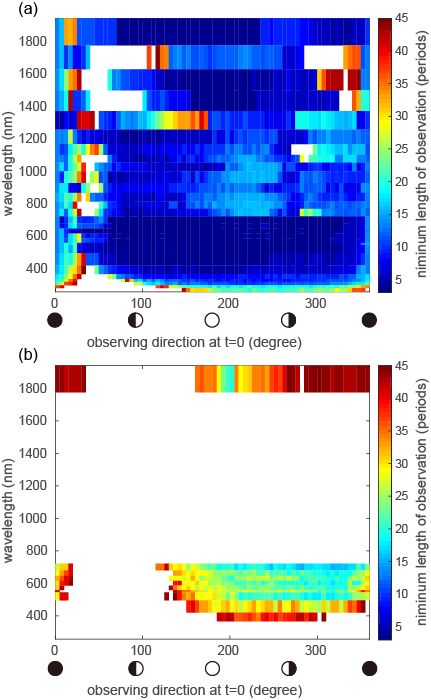
the wavelength, latitude, and longitude. To calculate a time series of the disc-averaged flux, we
first need to pick an observing direction. It should be noted that any observing direction is possible
for an unknown exoplanet. Therefore, we use two divergent sets of observing directions in our
analysis (Figure 1). In the first set of observing directions, the orbit of the exoplanet is edge-on in
the perspective of the observer (hereafter azimuthal-rotated edge-on). The transit configuration is
defined as 0°, while the secondary eclipse configuration is defined as 180° (see Figure 1a). In the
second set of observing directions (hereinafter referred as polar-rotated face-on), the exoplanet
stays in the plane generated by the observing direction and the normal direction of the orbit. The
face-on orbit with the northern/southern hemisphere exposed to the observer is defined as 0°/180°,
while the transit and secondary eclipse configurations are defined as 90° and 270°, respectively
(see Figure 1b). Once an observing direction and a specific wavelength range are picked, a time
series of the disc-averaged reflected solar flux can be calculated from the simulation results. The
original time resolution of the time series is 2 hours, which is the same as the time resolution of
the model output. By averaging nearby data points, the time resolution of the time series can be
arbitrarily decreased. We also add simulated observational errors to the time series in order to
mimic real observations.
   Figure 2a represents an example of a time series of simulated reflected starlight created from
the model output. In this case, we use the 1-Earth-day rotation period simulation output in the
wavelength range between 540 nm and 550 nm and the length of the time series is 25 days. The
observing direction is set at 220° of the azimuthal-rotated edge-on orbit and the time resolution is
2 hours. The standard deviation of the observational error is set to be 5% of the disc-averaged flux,
which approximately corresponds to a signal-to-noise ratio of 20 for the starshade-enabled
telescope. We also show the detrended time series, the Fast Fourier transform (FFT) of the
detrended time series, and the signal-to-noise ratio in Figure 2. The signal-to-noise ratio, which is
the power density of the signal divided by the variance of the observational error (Scargle 1982),
is calculated from the time series (shown in Figure 2d). To report a signal with high confidence
(low false alarm probability), the signal-to-noise ratio of the signal must exceed a certain threshold.
In Figure 2d, the red line represents the signal-to-noise ratio threshold calculated according to
Scargle (1982) to permit reporting a signal with 99% confidence. It should be noted that this
threshold is a function of the length of the time series. Based on Figure 2d, there are two signals
detected with >99% confidence (
second highest peaks are 1.0 day and 0.5 day, respectively. The 1.0-day signal corresponds to the
rotation period while the 0.5-day signal corresponds to the possible periodic patterns of land-ocean
or cloud distribution. We find it possible that the highest peak occurs at 0.5 day, 0.33 day or even
0.25 day rather than 1.0 day. Therefore, we propose the following algorithm to obtain the rotation
period from a time series:
       (1) Pick the highest peak in the FFT result, then check if the signal-to-noise ratio of this
           peak is above the 99% confidence threshold.
       (2) If not, then we consider that the rotation period cannot be detected from this time series.
           If yes, then check if there is another peak that is above the signal-to-noise threshold
           and has the period that is an integral multiple of the period of the highest peak.
       (3) If not, the rotation period we detect is the period of the highest peak. If yes, the rotation
           period we detect is this integral multiple of the period of the highest peak.
       (4) Finally, check if the rotation period we detect is the actual rotation period of the
           simulated exoplanet. If yes, we consider that the rotation period can be detected from
           this time series.
   With steps (1) to (4), we are able to determine whether the rotation period of the exoplanet can
be detected from a simulated time series. When we alter the parameters of the simulated
observation (e.g., observing direction, wavelength range, etc.), the time series and the detectability
of the rotation period change. In the next section, we will explore how different parameters
influence the detectability of the rotation period of an Earth-like exoplanet.

4. Sensitivity of the detectability of the rotation period to parameters
   To understand the conditions under which the rotation period of an Earth-like exoplanet is
likely to be detectable, here we consider 7 important factors that affect the observations.
4.1. Length of observation
   We find that generally it is easier to detect the rotation period with longer lengths of
observation. Figure 3 shows a time series that is obtained in the same condition as the time series
in Figure 2 except that the length of this time series is only 4 days. From Figure 3d, we clearly see
that this time series does not meet our criteria for rotation period detection. Therefore, under a
given condition, the minimum length of observation needed to detect the real rotation period is a
key parameter that measures the detectability of the rotation period.

                                                                                                      5
4.2. Rotation period
Since the detectability of the rotation period depends on how many periods are contained in
the time series, the minimum length of observation needed to detect the rotation period should be
measured in periods instead of days. In section 3, we used 1 per 2 hours, 1 per 4 hours, etc. to
represent the time resolution of the time series. A more sophisticated way to describe the time
resolution is the number of data points in one period. In other words, 1 per 2 hours for a 1-day
rotation period and 1 per 4 hours for a 2-day rotation period dataset are equivalent, each
corresponding to 12 data points per period. Ideally the minimum observation length needed to
detect the rotation period should be a constant number of rotational periods. However, our analysis
shows that sometimes the minimum length of observation (in rotational periods) needed for the 1-
day rotation period dataset and the minimum length of observation needed for the 2-day rotation
period dataset are not always equal. In what follows we will regard the minimum length of
observation needed to detect the rotation period under a given condition as the larger minimum
length of observation obtained from the two datasets.
4.3. Wavelength
The detectability of the rotation period may vary with the wavelength used to observe the
exoplanet. Here we fix the observing direction at 180° of the azimuthal-rotated edge-on orbit, the
time resolution at 12 data points per period and the observational error at 5%. We then calculate
the minimum length of observation needed to detect the rotation period for different wavelength
ranges (Figure 4.) If the rotation period cannot be obtained from an observational length of 45
rotation periods, we consider the rotation period to not be detectable under this condition. In Figure
4, we can see that the minimum length of observation needed in the visible channels (500 – 700
nm) is less than 10 periods, much shorter than the minimum length of observation needed for the
ultraviolet and near-infrared channels. This phenomenon is mainly due to the fact that the
reflectance of land, ocean and cloud are more diverse in the visible channels than in other channels
(Xu et al., 2015; Kokaly et al., 2017).
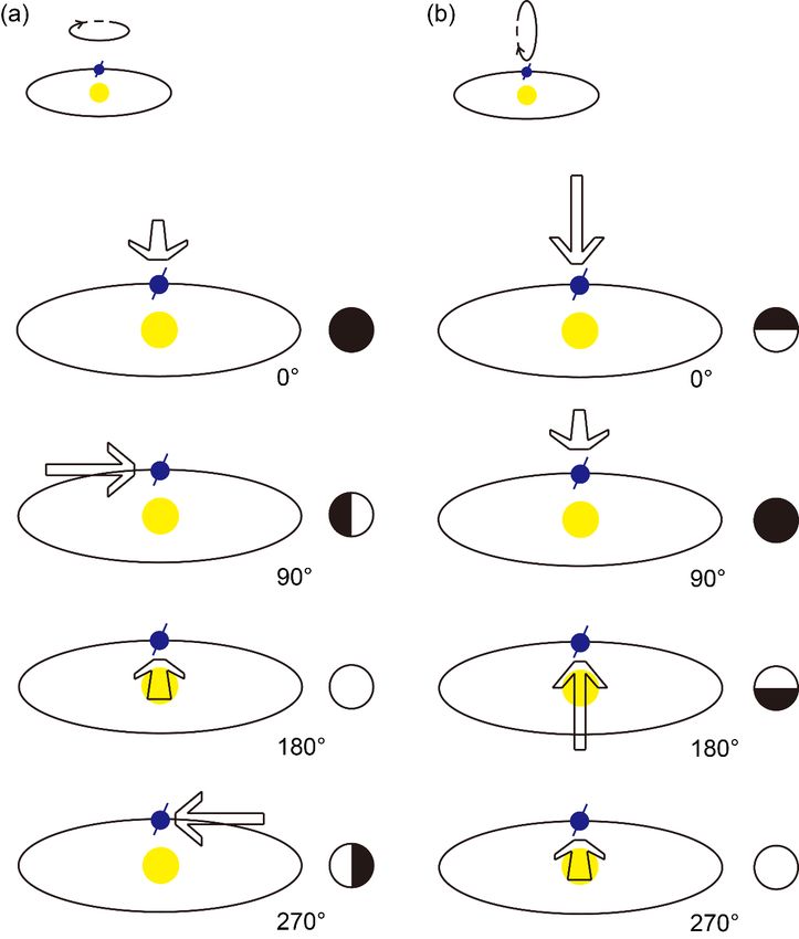
4.4. Observing directions
If the exoplanet is near secondary eclipse, the observer can see almost the entire sunlit disc (as
long as the star is not blocking the planet) which will maximize the variation in reflected light. If
the exoplanet is near transit, the observer can see very little reflected starlight from the exoplanet,
which will minimize the variation in reflected light. Therefore, the observing direction clearly
6influences the detectability of the rotation period. We fix the time resolution at 12 data points per
period and the observational error at 5%, then find the minimum length of observation needed to
detect the rotation period as a function of wavelength and observing direction (shown in Figure 5).
For the near infrared channels below 1.3 µm, in a range of ~100° in both azimuthal and polar angle
around the secondary eclipse, the rotation period is detectable with ~20-30 periods of observation.
In the visible channels, the rotation period is detectable with less than 15 periods of observation in
a much larger direction range. As expected, the rotation period of the exoplanet is only hard to
detect near transit. For the ultraviolet channels above 285 nm, the rotation period is detectable near
the secondary eclipse with more than 25 periods of observation. The rotation period is undetectable
at wavelengths less than 285 nm.
4.5. Time resolution
To evaluate the influence of time resolution on the detectability of the rotation period, we
repeat the analysis from section 4.4 with coarser time resolutions of 6 data points per period (Figure
6a), 4 data points per period (Figure 6b), and 3 data points per period (Figure 6c). With 6 data
points per period, the rotation period is still detectable in a large direction range in visible channels,
but the minimum length of observation needed to detect the rotation period becomes about 2 times
longer than the higher resolution scenario (Figure 6a). In contrast, the rotation period becomes
undetectable at other wavelengths. If the time resolution is decreased to 3 data points per period,
the rotation period is only detectable near transit (Figure 6c). This is consistent with Jiang et al.
(2018), who showed that when the time resolution is lower than 2 per period, the probability of
detecting the rotation period drops dramatically.
4.6. Observational error
In the previous analysis, we fixed the standard deviation of the observational error added to
the time series at 5% of the disc-averaged flux, which approximately corresponds to a signal-to-
noise ratio (S/N) of 20 for each integration. To evaluate the influence of the S/N on the detectability
of the rotation period, we recreate our analysis from section 4.4 but change the S/N to 40 and 10
(Figure 7),. When the S/N is 40, the detectability is significantly enhanced in all channels (Figure
7a). In the visible and near-infrared channels, the minimum length of observation needed to detect
the rotation period is less than 10 periods for most of the observing directions. Moreover, even the
ultraviolet channels below 285 nm become detectable. On the contrary, when the S/N is 10 (Figure
7b), the rotation period is undetectable for most of the ultraviolet and near-infrared channels.
7Although the rotation period is still detectable for the visible channels, it requires more than 20 to 25 periods of observation. 4.7. Land fraction The fractions of land and ocean on Earth’s northern hemisphere are comparable, whereas on Earth’s southern hemisphere the ocean covers more than 80% of the surface. Therefore, the southern hemisphere of the Earth is more like an aqua planet (i.e., a planet with full ocean coverage) instead of an Earth-like planet. We can exploit this asymmetry to investigate how land fraction influences the detectability of the planetary rotation period. For example, when the observer focuses on the northern hemisphere (observing direction around 0°), the rotation period is detectable for most of the channels (Figure 5b). In contrast, when the observer focuses on the southern hemisphere (observing direction around 180°), the rotation period becomes undetectable. This result implies that the rotation period of an exoplanet with no land is unlikely to be detected using the observational technique outlined here. In other words, an exoplanet whose rotation period can be detected is likely to have a mix of continents and ocean, which may be used to infer information about the planet’s geophysical and geochemical context that would otherwise be hidden. 5. Conclusion and discussion In this study, we simulate observations of ExoCAM output to evaluate the detectability of a terrestrial exoplanet’s rotation period through an FFT analysis of reflected starlight. Our work shows that to better detect the rotation period, one needs to plan the observation so that each individual integration would yield a S/N >10, while keeping the integration time shorter than 1/6 – 1/4 of the rotation period of the planet. The best wavelength to carry out this observation will be in 500 – 700 nm, and in this wavelength, the rotation period may be obtained with an observation campaign that lasts for ~10 rotation periods. Using Earth as an analog, the quantities above correspond to repeating the integration of
number per period and the length of the time series to a multiple of the rotation periods. By
comparing the parameters of the observation (time resolution, S/N, length of observation, etc.) to
the parameter space explored in Section 4, one can tell whether this preliminary rotation period is
likely to be the true rotation period or not.
    Future space telescopes in planning may provide the required conditions to detect the rotation
periods of terrestrial planets in the habitable zone of some nearby stars. For example, a HabEx-
like telescope would achieve an S/N=20 per 5-nm spectral channel in 500 – 700 nm for an Earth-
like planet in the habitable-zone of the nearest stars (distance < 4pc, e.g., tau Ceti, epsilon Indi A)
in ~10 hours (Hu et al. 2021). This translates to an integration time of ~6 hours per ~10-nm spectral
channel, corresponding to the simulation shown in this paper. The rotation period would thus be
detectable if Earth analogs are found in these systems and ~10 days of the mission time are
dedicated to the campaign. Given the importance of the rotation period (it is one of the basic
planetary parameters aside from mass and radius) and possible science that can be achieved at the
same time (e.g., surface composition mapping, Cowan et al. 2009; Fan et al. 2019), a ~10-day
campaign may be palatable. The requirement will be less stringent for planets larger than Earth or
closer to their host star, for which the endeavor to detect the planetary rotational period may be
extended to stars further away. A larger space telescope (e.g., the LUVOIR mission concept)
would enable rotation period detection in more systems.
    In Section 4.7, we proposed that the rotation period of an aqua exoplanet is likely undetectable.
However, this is based on the precondition that we only have photometric observations of the
exoplanet. Ocean glints, which have been shown to facilitate surface mapping of potential
habitable exoplanets (Lustig-Yaeger et al., 2018), are highly polarized. Kopparla et al. (2018)
model the polarization signal of the TRAPPIST-1 system and show that the polarization signal
from an ocean-covered exoplanet is stronger and easier to detect than the intensity signal. If a
direct-imaged polarization observation of an exoplanet is available, the rotation period of an aqua
exoplanet may still be detectable. A polarization observation may also improve the detectability
of the rotation period of Earth-like exoplanets.
    In this paper, we have studied fast-rotating exoplanets, whose rotation period is much smaller
than its orbital period. For the Venus-like, slow-rotating exoplanets whose rotation period is
comparable to the orbital period, the variation of the reflected starlight caused by its rotation will

                                                                                                     9
be coupled with the variation caused by its revolution so that the signal of the rotation period may
be hard to detect. Further studies are required to address this problem.
In summary, we find that it will be possible to detect the rotation period of a terrestrial
exoplanet using direct imaging if the planet is observed in favorable conditions. The detection of
the rotation period of Earth-like exoplanets will help us identify habitable exoplanets and provide
us information on the dynamical evolution of exoplanetary systems.
Acknowledgement
We thank Eric Wolf for developing, maintaining, and making publicly available ExoCAM.
This work is supported by the Jet Propulsion Laboratory, California Institute of Technology, under
contract with NASA. We also acknowledge the funding support from the NASA Exoplanet
Research Program NNH18ZDA001N-2XRP. This work was supported by the NASA
Astrobiology Program grant No. 80NSSC18K0829 and benefited from participation in the NASA
Nexus for Exoplanet Systems Science research coordination network.
Data Statement
The ExoCAM model source code and related data are available to download from
https://github.com/storyofthewolf/ExoCAM. The computed data underlying this article are
described in the article. For additional questions regarding the data and code sharing, please contact
the corresponding author.
References
Aizawa, M., Kawahara, H., & Fan, S. (2020). Global mapping of an exo-Earth using sparse
modeling. The Astrophysical Journal, 896, 22.
Barnes, R. (2017). Tidal locking of habitable exoplanets. Celestial Mechanics and Dynamical
Astronomy, 129, 509.
Bitz, C. M., Shell, K. M., Gent, P. R., et al. (2012). Climate sensitivity of the community climate
system model, version 4. Journal of Climate, 25, 3053.
Brogi, M., De Kok, R. J., Albrecht, S., et al. (2016). Rotation and winds of exoplanet HD 189733
b measured with high-dispersion transmission spectroscopy. The Astrophysical Journal, 817,
106.
Cash, W. (2006). Detection of Earth-like planets around nearby stars using a petal-shaped
occulter. Nature, 442, 51.
Fan, S., Li, C., Li, J. Z., et al. (2019). Earth as an exoplanet: A two-dimensional alien map. The
Astrophysical Journal Letters, 882, L1.
10Forget, F., & Leconte, J. (2014). Possible climates on terrestrial exoplanets. Philosophical
Transactions of the Royal Society A: Mathematical, Physical and Engineering Sciences, 372,
20130084.
Gu, L., Fan, S., Li, J., et al. (2021). Earth as a Proxy Exoplanet: Deconstructing and Reconstructing
Spectrophotometric Light Curves. The Astronomical Journal, 161, 122.
Haqq-Misra, J., Wolf, E. T., Joshi, M., et al. (2018). Demarcating circulation regimes of
synchronously rotating terrestrial planets within the habitable zone. The Astrophysical
Journal, 852, 67.
Hess, S. L. G., & Zarka, P. (2011). Modeling the radio signature of the orbital parameters, rotation,
and magnetic field of exoplanets. Astronomy & Astrophysics, 531, A29.
Hu, R., Lisman, D., Shaklan, S., et al. (2021). Overview and reassessment of noise budget of
starshade exoplanet imaging. Journal of Astronomical Telescopes, Instruments, and
Systems, 7, 021205.
Jiang, J. H., Zhai, A. J., Herman, J., et al. (2018). Using deep space climate observatory
measurements to study the Earth as an exoplanet. The Astronomical Journal, 156, 26.
Kaspi, Y., & Showman, A. P. (2015). Atmospheric dynamics of terrestrial exoplanets over a wide
range of orbital and atmospheric parameters. The Astrophysical Journal, 804, 60.
Kasting, J. F., Whitmire, D. P., & Reynolds, R. T. (1993). Habitable zones around main sequence
stars. Icarus, 101, 108.
Kokaly, R. F., Clark, R. N., Swayze, G. A., et al. (2017). USGS spectral library version 7 (No.
1035). US Geological Survey.
Komacek, T. D., & Abbot, D. S. (2019). The atmospheric circulation and climate of terrestrial
planets orbiting Sun-like and M dwarf stars over a broad range of planetary parameters. The
Astrophysical Journal, 871, 245.
Kopparapu, R. K., Wolf, E. T., Haqq-Misra, J., et al. (2016). The inner edge of the habitable zone
for synchronously rotating planets around low-mass stars using general circulation
models. The Astrophysical Journal, 819, 84.
Kopparapu, R. K., Wolf, E. T., Arney, G., et al. (2017). Habitable moist atmospheres on terrestrial
planets near the inner edge of the habitable zone around M dwarfs. The Astrophysical
Journal, 845, 5.
Kopparla, P., Natraj, V., Crisp, D., et al. (2018). Observing Oceans in Tightly Packed Planetary
Systems: Perspectives from Polarization Modeling of the TRAPPIST-1 System. The
Astronomical Journal, 156, 143.
Lustig-Yaeger, J., Meadows, V. S., Mendoza, G. T., et al. (2018). Detecting ocean glint on
exoplanets using multiphase mapping. The Astronomical Journal, 156, 301.
11May, E. M., Taylor, J., Komacek, T. D., et al. (2021). Water Ice Cloud Variability and Multi-epoch
Transmission Spectra of TRAPPIST-1e. The Astrophysical Journal Letters, 911, L30.
Rasch, P. J., & Kristjánsson, J. E. (1998). A comparison of the CCM3 model climate using
diagnosed and predicted condensate parameterizations. Journal of Climate, 11, 1587.
Scargle, J. D. (1982). Studies in astronomical time series analysis. II-Statistical aspects of spectral
analysis of unevenly spaced data. The Astrophysical Journal, 263, 835.
Showman, A. P., Wordsworth, R. D., Merlis, T. M., et al. (2013). Atmospheric circulation of
terrestrial exoplanets. Comparative Climatology of Terrestrial Planets, 1, 277.
Snellen, I. A., Brandl, B. R., de Kok, R. J., et al. (2014). Fast spin of the young extrasolar planet β
Pictoris b. Nature, 509, 63.
Vanderbei, R. J., Cady, E., & Kasdin, N. J. (2007). Optimal occulter design for finding extrasolar
planets. The Astrophysical Journal, 665, 794.
Way, M. J., Del Genio, A. D., Kiang, N. Y., Sohl, L. E., Grinspoon, D. H., Aleinov, I., ... & Clune,
T. (2016). Was Venus the first habitable world of our solar system?. Geophysical research
letters, 43(16), 8376-8383.
Wolf, E. T., & Toon, O. B. (2015). The evolution of habitable climates under the brightening
Sun. Journal of Geophysical Research: Atmospheres, 120, 5775.
Wolf, E. T., Shields, A. L., Kopparapu, R. K., et al. (2017). Constraints on climate and habitability
for Earth-like exoplanets determined from a general circulation model. The Astrophysical
Journal, 837, 107.
Wolf, E. T. (2017). Assessing the habitability of the TRAPPIST-1 system using a 3D climate
model. The Astrophysical Journal Letters, 839, L1.
Xu, M., Pickering, M., Plaza, A. J., et al. (2015). Thin cloud removal based on signal transmission
principles and spectral mixture analysis. IEEE Transactions on Geoscience and Remote
Sensing, 54, 1659.
Yang, J., Boué, G., Fabrycky, D. C., et al. (2014). Strong dependence of the inner edge of the
habitable zone on planetary rotation rate. The Astrophysical Journal Letters, 787, L2.
Yang, J., Abbot, D. S., Koll, D. D., et al. (2019). Ocean dynamics and the inner edge of the
habitable zone for tidally locked terrestrial planets. The Astrophysical Journal, 871, 29.
12Figure 1. Two divergent sets of observing directions used in this study. On the top of each panel,
the small diagram shows how we rotate the orbit to obtain different observing directions. The
diagrams below show the correspondence between the angles and the observing directions. (a)
The exoplanet is in an azimuthal-rotated edge-on orbit. (b) The exoplanet is in a polar-rotated
face-on orbit. The markers next to each diagram represent the orientation of the sunlit disc in the
view of the observer.
13Figure 2. How we derive the rotation period from a time series. (a) A simulated time series of
reflected star light for the 1-day rotation period experiment. (b) The detrended time series. (c)
Fourier transform of the detrended time series. (d) Signal-to-noise ratio as a function of period.
The red line indicates the signal-to-noise threshold for 99% confidence.
14Figure 3. As Figure 2, except the length of the time series is 4 days. The 99% confidence
threshold in panel (d) is lower than the threshold in Figure 2d due to the shorter time series.
15Figure 4. An example of the minimum length of observation needed to detect the rotation period
as a function of wavelength. We combine 1 and 2 day period data here (see section 4.2) and use a
99% confidence threshold. The observing direction is 180° of the azimuthal-rotated edge-on
orbit, the time resolution 12 data points per period, and the observational error is 5%.
Figure 5. The minimum length of observation needed to detect the rotation period as functions
of the wavelength and observing direction. We combine 1 and 2 day period data here (see section
4.2) and use a 99% confidence threshold. The time resolution is 12 data points per period. The
observational error is 5%. (a) Azimuthal-rotated edge-on orbit observing directions (see Figure
161). (b) Polar-rotated face-on orbit observing directions. The color white indicates that the rotation
period is not detectable.
17Figure 6. (a) Same as Figure 5a, except that the time resolution is 6 data points per period. (b)
Same as Figure 5a, except that the time resolution is 4 data points per period. (c) Same as Figure
5a, except that the time resolution is 3 data points per period.
18Figure 7. (a) Same as Figure 5a, except that the S/N is 40. (b) Same as Figure 5a, except that the
S/N is 10.
19You can also read