The Demand for EuroMillions Lottery Tickets

The Demand for EuroMillions Lottery Tickets:

An International Comparison1

Patrick Roger
LARGE, Université de Strasbourg, EM Strasbourg Business School, 61 Avenue de la Forêt Noire, 67085
Strasbourg Cedex, France
e-mail proger@unistra.fr

           Abstract
           In this article, we analyze the demand for EuroMillions tickets, a European
           lottery game launched in 2004 and played simultaneously in nine countries with
           the same rules and the same draws. Firstly, using the effective price methodology,
           we show that price elasticities are very different across countries. In particular,
           Spain and Portugal exhibit low price elasticity and high mean sales, meaning a
           low sensitivity to jackpot increases. Ireland and the United Kingdom on the other
           hand, exhibit very high long-run elasticity and a large sensitivity to jackpot
           variations. The interpretation of these results is linked to lower per capita GDP in
           the first two countries, to the development of much syndicated gaming in Spain,
           and to the special tax regime in Portugal. Bookmaking activities and the highly
           competitive betting market in the UK and Ireland partly explain the results. We
           then show that cumulative prospect theory (Tversky and Kahneman (1992)),
           though allowing participation in the lottery to be explained, does not improve the
           estimation of the demand function.
           Classification JEL : D81, H71

1
    I wish to thank Serge Blondel, Jalal El Ouardighi, Bertrand Koebel, Jean-Marc Tallon (editor), two anonymous
    referees, and my colleagues in the laboratory LARGE for their comments and suggestions that have allowed me to
    improve earlier versions of this article.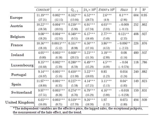

Introduction

E        uroMillions is a lottery launched in February 2004 in three countries, Spain,

France, and the United Kingdom. In October 2004, six other countries joined the pool:
Austria, Belgium, Ireland, Luxembourg, Portugal, and Switzerland. The main feature of
this lottery is a very low probability of winning the jackpot, approximately one chance in
76 million.2

To offer a single game on the European scale allows the pool of potential players to be
increased and prevents players from experiencing jackpot fatigue when faced with the
absence of winners, in particular in countries with small populations (Matheson and
Grote 2004). In fact, when it seems “impossible” to win the jackpot, the players abandon
the game, which increases the probability that there will not be a winner in the next
draw and ends up putting the survival of the game at risk.

On the other hand, a low probability of winning produces rollovers, i.e., the carrying
forward of jackpots not won from one drawing to the next. Rollovers produce two
conflicting effects. On the one hand, the game is more attractive when the jackpot
increases, while on the other hand, the probability of sharing the jackpot in the case of a
win also increases, which decreases the amount received by the winner.

The demand for lottery tickets is traditionally estimated by the effective price method.
The effective price is calculated as the difference between the cost of the ticket and its
expected value.3 The cost is known and generally stable over time, while the expected
value changes at each drawing for two reasons. The first is the existence of rollovers,

2
    EuroMillions is one of the lotteries having the lowest probability of winning the jackpot.
3
    Cook and Clotfelter (1993), Farrell et al. (1999), Forrest et al. (2000, 2002, 2008), Forrest and McHale (2007),
    Geronikolaou and Papachristou (2007), Gulley and Scott (1993), Mason et al. (1997), Purfield and Waldron
    (1999), Walker (1998), Wang et al. (2006).

which increase the expected value and reduce the effective price. The second, which is
not independent of the first, comes from the fact that the effective price depends on the
number of tickets sold, a number which influences the probability of rollover. The
method of estimation must take these two effects into account. These remarks show that
the estimation of the demand function for EuroMillions tickets presents a particular
interest because of the very low probability of winning and the numerous rollovers.4

The second interest of the present article comes from the international character of the
lottery that is played in nine countries with the same rules, draws and rollovers. To our
knowledge, there is no other comparable study, since international comparisons of
lotteries treat games which differ across countries (Garrett 2001). In this article, we
analyze the demand for tickets on the European level, then country by country,
examining two preference hypotheses. The first assumes the linearity of preferences
with respect to probabilities and is the most common hypothesis in the literature,
associated with the effective price method mentioned previously. However, it does not
allow participation in the game to be justified since the expected profitability of the
game is largely negative. The second preference hypothesis consists in assuming that the
objective probabilities are distorted in such a way that the perceived probability of
winning the jackpot is largely overestimated. This alternative is in line with the
hypothesis of the transformation of probabilities that one can find notably in Prospect
Theory (Kahneman and Tversky 1979; Tversky and Kahneman 1992) or in the rank-
dependent expected utility model (Quiggin 1982). It enables the demand to be estimated
but also the participation in an unfavorable lottery to be justified,5 since this objective is
not achieved in the classic model.

4
    67.9 % of the drawings did not produce a jackpot winner between February 2004 and October 2008 (239
    drawings). Even if the period is reduced, beginning in October 2004 (when six new countries entered), the
    percentage is still 66.66%. In addition, two sequences of 12 consecutive drawings without a winner occurred
    during this period.
5
    The first attempts to resolve this problem introduced convex parts into the utility function (Friedman and Savage
    (1948), Markowitz (1952)). Earlier models, widely used today, are based on the distortion of objective
    probabilities.

One can note that certain authors attribute a “use value” to the very fact of playing, by
interpreting participation in a game such as the lottery or EuroMillions as the purchase
of a “right to dream”(Conlisk 1993; Forrest et al. 2002; Quiggin 1991). With this
perspective, Kearney (2005), analyzed the effects of substitution between lotteries and
other consumer goods and showed that the spending dedicated to lotteries did not
substitute that for other games of chance, but in fact for spending on other consumer
goods. Whichever hypothesis is adopted, the distortion of probabilities or the purchase
of a dream, it largely involves the over-weighting of the jackpot when evaluating the
lottery. This is why we also estimate the demand functions by replacing the effective
price by the anticipated level of the jackpot, according to the model used by Forrest et al.
(2002). We shall see however, that this approach does not improve the quality of the fit
which is already very good in the standard approach. We assume, however, a different
behavior for the player since, on the one hand, there is a classic price-demand relation,
while on the other, the larger the quantity of the desired characteristic in the product
(amount of the jackpot), the more the player is ready to pay.

In this article, we demonstrate significant behavioral differences between countries. In
particular, we show that players in the United Kingdom are very sensitive to variations
of the jackpot (which corresponds to a decrease in the effective price, real or perceived,
depending upon whether the probabilities are objective or deformed). The very
competitive games environment that characterizes the United Kingdom can comprise an
important reason for the higher sensitivity of players in this country, as recently
demonstrated by Forrest et al. (2008). On the other hand, Spanish and Portuguese
players are much less sensitive to these variations. Several explanations can be
advanced. Differences in GDP per capita can constitute a first explanation for this
surprising result. In fact, lotteries are often described as regressive taxation, hitting
most particularly the low-income categories (Oster 2004).

The culture of syndicated gaming (players play as a group) in Spain also leads to lower
sensitivity, given the transaction and information-related costs between members of the
group. Lastly one should note that, in Portugal, the winnings from all lotteries, with the

exception of EuroMillions, are taxed,6 which can explain the very high level of
participation and the lower sensitivity to variations of the jackpot.

On the European level, we obtain a long-run price elasticity equal to -0.9, which is
consistent with most of the results in the literature. Farrell et al. (1999) obtained an
elasticity of -1.05 for the United Kingdom, Forrest et al. (2002), -0.82, and Forrest and
McHale (2007), -0.91 for the most recent data. With regard to studies of American
lotteries, Gulley and Scott (1993) obtained elasticities equal to -1.15, -1.92, and -1.2 for
the lotteries of Massachusetts, Kentucky, and Ohio. On the other hand, we shall show
that there are large disparities between countries participating since the same
elasticities vary from -0.49 for Spain to -1.76 for the United Kingdom.

Farrell et al. (1999) interpreted the coefficient of lagged sales in the demand equation as
a measurement of the addictive character of the lottery. They obtained a coefficient of
0.33 for the United Kingdom lottery between November 1994 and February 1997. There
again, with respect to EuroMillions, the results vary considerably from one country to
another since the estimated coefficients vary from 0.2 for Spain to 0.67 for Ireland.

The article is organized as follows. Section 2 summarizes the EuroMillions rules and
presents the data used in the empirical study. Section 3 is dedicated to two models for
estimating the demand, according to the hypothesis adopted for preferences. The
empirical results at the European level are presented in section 4, while in section 5, the
results are detailed country by country. A final section provides conclusions and
proposes directions for further research.

6
    We wish to thank an anonymous referee for having drawn our attention to this point.

EuroMillions Rules and Data Used

EuroMillions Rules

To fill in a EuroMillions ticket, the player first chooses five different numbers between 1
and 50, and then, in the second group, two different numbers between one and nine.
These two numbers are in general called “stars” in reference to the European flag.7

EuroMillions offers 12 ranks of winning that are summarized in table 1. The notation
n+m signifies that n correct numbers have been chosen in the first group of 50 numbers
and that m correct numbers come from the group of nine stars.

       Table 1: Ranks of Winning, Distribution of Prizes, and Probabilities of
                                                     Winning

The column “% prize” gives a distribution of winnings according to the rank of winning
at the end of the study period. This distribution has been twice modified since the
launching of the game. The proportion reserved for rank 1 was initially 20%. It changed
to 22% in August 2004, and then reached its current level of 32% in February 2006.
This distribution is common in lotteries. The portions of the first and last ranks are
always large, but the reasons are different. A high jackpot makes the game attractive and
the existence of numerous “small winners” avoids discouraging players from betting on
the following drawing. One can expect therefore that the sales for a given drawing

7
    Lotteries are generally based on the drawing of 5 to 7 numbers in groups of 35 to 55 numbers.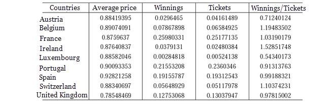

influence the sales for the following drawing since the global amount of these
consolation prizes is proportional to the sales.

EuroMillions also distinguishes itself from other lotteries by its international character
since it is played in nine countries under the same conditions with a single drawing. All
players face the same rules.8 We should mention however, that the cost of the ticket is
2 € in the euro zone, £1.5 in the United Kingdom, and 3.2 francs (CHF) in Switzerland.
As the tickets and the winnings are expressed with the same currency, we consider that
all of the amounts are euro-equivalent. It is the most natural choice since the countries
of the euro zone are the most numerous, and this presents an additional advantage
where the withholding of the organizer is 50%,which leads to equality in the number of
tickets with the amount redistributed (apart from rollovers).

Coming back to table 1, it is noted that the sum of the percentages of winning is only
94%. This is explained by the existence of a reserve fund intended to supply certain
jackpots. In fact, when the jackpot has just been won, the following one is generally 15
million, and it requires a volume of 46 million tickets sold to ensure the payment,9
which is much greater than the average sales.

When a jackpot is not won, (rollover), the amounts reserved at this rank (32% of total
winnings) will feed the jackpot for the following drawing, as well as a portion of the
reserve fund. The organizers of the game communicate the estimated amount of the
following jackpot with heavy radio, television, or print media advertising. Even if it is
not possible to obtain the exact amounts dedicated to these ads, it is obvious that this
communication has an effect on sales, in particular when the jackpot reaches very high
amounts after five or six rollovers. However, it is not so much the budget dedicated to
communication as the message itself that influences sales, this message in every case
summing up the single amount of the following jackpot.

8
    It should be mentioned that winnings of the game are not taxed, except in Switzerland where the withholding at
source is 35%.
9
    When the game started, and only three countries participated, there were several jackpots of €10 million.

Certain exceptional events also give rise to more intense advertising communication.
This is the case when exceptional jackpots are offered, which are not the result of a
series of rollovers. As we will stipulate further, our study period contained two events of
this type, with respective jackpots of 100 and 130 million euros. These cases receive a
special treatment in the demand estimation model.

In summary, EuroMillions is the ideal lottery for an international comparison since
numerous variables are controlled. The takeout rate by the organizer is the same in
every country; in addition, it has stayed constant since the beginning of the game. This
is not the case in other international comparisons appearing in the literature (e.g.,
Garrett 2001). Consequently, if differences appear in the demand functions, they cannot
come from the design of the game, but are rather a consequence of behavioral
differences or differences related to the environment of the game.

The Data
Our database is constructed from the site www.sojah.com, which is the official site
regarding games of chance organized in France. It supplies time series of drawings and
individual winnings, but also all the legal texts with regard to lotteries. Concerning
EuroMillions, this site allows access to the data of all participating countries.

Our database includes the first 197 drawings, from the day of launch (February 13,
2004) until    November 16, 2007. We have mentioned in the introduction that six
countries joined the first three at the 35th drawing. Consequently, we eliminate these
first 35 drawings, including the day of entry of the six new countries, to avoid the bias
induced by the attractiveness of the first drawing (increased by advertising
communication related to the launch) for the players of these six countries. Finally, 162
drawings are included in the analysis that follows, starting on October 15, 2004.

The following data will be used:
    the volume of sales, country by country, and the aggregate level;

      the individual winnings for each rank of winnings;
       the number of players winning at each rank, and in each country;
       the effective jackpot (known only after the drawing), which is divided between the
        first-rank winners;
       the percentage of winnings reserved at each rank.10

It is worth noting that more than 80% of sales are made in four countries, Spain,
France, Portugal, and the United Kingdom. In addition, Portugal, with only 11 million
inhabitants, realizes a turnover comparable to that realized in France and in Spain and
greater than that in the United Kingdom, while the population of these countries is five
or six times higher. We will come back to this point below.

Descriptive Statistics
Table 2 presents the descriptive statistics with regard to the essential variables entering
into the estimation of the demand function, i.e., weekly sales, anticipated jackpot (the
calculation of which will be detailed in the following section), and the actual jackpot as it
appears in the database. In columns 2 and 3, we have added the populations of the
countries and the GDP per capita.11

        Table 2: Descriptive Statistics of the Population, the GDP Per Capita,
                                              and Weekly Sales*

10
     This distribution underwent a single change during our study period. The portion reserved for the jackpot shifted
     from 22 to 32%. This modification was compensated for by a decrease in the percentage dedicated to the reserve
     fund, which shifted from 16 to 6%.
11
     These data are given in 2006 $US and come from the website of the Conference Board and the Groningen Growth
     and Development Centre (http://www.conference-board.org/economics/database.cfm).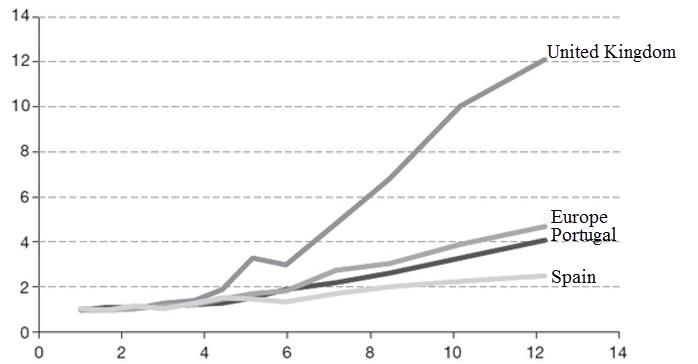

For variables concerning the game itself, the table gives the following variables:
minimum (Min), maximum (Max), mean (μ), standard deviation (σ), and coefficient of
variation (μ/σ). As we’ve already mentioned, the range of variation is very broad,
essentially due to rollovers.

Several elements in the table are worth commenting upon, in particular, the situations
of Portugal, the United Kingdom, and Luxembourg. Portugal is characterized by a high
average level of sales, particularly if one considers the population, and by a low
coefficient of variation of 0.38 (however, the coefficient for Spain is even lower). On the
other hand, the United Kingdom is remarkable because of the low average level of sales,
(there again with respect to the population) and a very high coefficient of variation.

The two countries for which the GDP per capita is the lowest (Spain, Portugal) also have
the lowest coefficient of variation. Knowing that the variations of sales from one week to
another are essentially due to rollovers, a possible interpretation of this fact is that the
players of the countries with low GDP are less sensitive to variations of the jackpot. This
can be explained by the fact that the initial jackpot is 15 million, which already
constitutes a very high amount for a low-income player. For example, the GDP per

capita of Portugal is equal to half that of Ireland, while its sales are three times higher.
In other words, a win of 15 million moves low-income players to wealth levels where the
marginal utility is negligible, or at least very low. In addition, lotteries are considered as
regressive taxation (Oster 2004) since they impact low-income populations.

Let us recall, however, that the situation of Portugal is very special as the winnings of
EuroMillions are not taxed, unlike those of other national lotteries. This can also be a
factor in the popularity of EuroMillions in Portugal.

Figures 1 and 2 illustrate the influence of the jackpot on sales and its variation across
(selected) countries, during two sequences of 12 consecutive weeks without a jackpot
winner.

       Figure 1: Standardized Sales as a Function of the Amount of the
      Jackpot, after 12 Drawings without a Jackpot Winner in Portugal,
             Spain, the United Kingdom, and Europe (9 Countries)
                     Sequence 1: November 18, 2005, to February 3, 2006

The initial level of sales is normalized to 1 for each country and represents the sales
when the jackpot is 15 million euros. In each of these figures, the Spanish and
Portuguese curves are situated below the average (corresponding to the aggregate level

for Europe), while the curve for the United Kingdom is situated largely above the
average. This shows the significant differences in sensitivity to the increase of the
jackpot in each of these countries.

The case of the United Kingdom is special in that gaming activities (gambling)
constitute a very competitive market. There were 680 authorized bookmakers in 2006,
according to the NJPC report (National Joint Pitch Council). When the jackpot increases
(and therefore the effective price decreases), EuroMillions becomes more competitive
compared to other lotteries, or more generally compared to other forms of gambling
(horseracing, dog racing, or sports gambling) proposed by bookmakers (Forrest et al.
2008).

         Figure 2: Standardized Sales as a Function of the Amount of the
      Jackpot, after 12 Drawings without a Jackpot Winner in Portugal,
            Spain, the United Kingdom, and in Europe (9 Countries)
                   Sequence 2: September 1, 2006, to November 17, 2006

Finally, the situation of Luxembourg is also worth noting. Table 2 shows that GDP per
capita is exceptionally high since it is 50% higher than that which immediately follows,

Ireland, and three times higher than that of Portugal. These data however, must be
considered with caution as thousands of bank and insurance company employees work
in Luxembourg, while they are French, Belgian, or German residents and cross the
border every day to go to work. This also indicates that it is impossible to identify the
origin of the sales. It could be that a non-negligible portion of these sales come from
cross-border workers.

Estimation of the Demand for EuroMillions Tickets

Specification of the Models

Linear Preferences with Regard to Probabilities

The usual method for estimating lottery sales is based on standard economic theory
linking price and demand. However, the cost of the ticket is very stable over time (and
even constant during our study). Therefore, it is not a good measure of price, simply
because each ticket can also be seen as an investment characterized by an expected
payoff. Because of this, most articles link demand to the effective price, defined as the
difference between the cost of the ticket and its expected payoff (Gulley and Scott 1993;
Scott and Gulley 1995; Walker 1998; Farrell et al. 1999; Forrest et al. 2001; Forrest et al.
2002; and Wang et al. 2006). The expected payoff is calculated here with respect to
objective probabilities. Consequently a lowering of the effective price by one cent has the
same effect whether the decrease is the result of an increase in the jackpot or the
increase in the winnings of the intermediate ranks. This is why we have mentioned
linearity with respect to probabilities in the title of this subsection. In the following
subsection, we will discuss the case where players distort objective probabilities.

The two principal factors determining the effective price are the volume of sales and the
rollovers which increase the jackpot and decrease the price. Other factors may influence
demand, such as the earnings of potential players or other demographic considerations.
However, in the short run, these factors are stable and do not explain the variations in
demand observed in Figure 3. This figure shows the evolution of ticket sales between

October 15, 2004, and November 16, 2007, i.e., 162 drawings. Considerable variations
appear, either progressively and in a few weeks, when several rollovers occur in a row,
or abruptly when an exceptional jackpot is offered. This is the case on two occasions
corresponding to drawings 122 (February 9, 2007, with a jackpot of 100 million) and 155
(September 20, 2007, with a jackpot of 130 million). These two points are circled in
Figure 3.

         Figure 3: Evolution of Sales over Time (in Number of Tickets)

This time-series of sales is typical of a lotto-like game (see for example Farrell et al.
1999; Gulley and Scott 1993; Purfield and Waldron 1999; or Beenstock and Haitovsky
2001). The successive rollovers lead to significant increases in sales, and Figures 1 and 2
have shown that the sales curve is growing and convex over the sequences of drawings
when the jackpot was not won. Beyond the jackpot effect, one can also observe a positive
trend in the evolution of sales since our study period began immediately after the game
was launched. The number of tickets evolves from 20 million at the start of the period to
40 million at the end of it.

Figure 4 shows the evolution of the jackpot over the same period. It is clearly apparent
that the sales peaks correspond to the highest jackpots, whether these come from

rollovers or from exceptional events (which are also circled in Figure 4). In fact, the
correlation between these two series is 0.89.

               Figure 4: Evolution of the Jackpot over Time (in €)

Finally, the growth of sales due to rollovers leads implicitly to a lower probability of
observing a rollover in the following drawing. Consequently, the amount of the rollover
is an essential determinant of the volume of sales, in as much as there is no longer any
withholding by the organizer on the rollover since it was already taken.

The pari-mutuel betting component of the game makes the estimation of demand
interesting in itself, because demand depends on effective price, itself determined by the
number of tickets sold (i.e., the demand). Therefore, the problem is resolved in two
steps. In the first step, the effective price is estimated from instrumental variables
influencing the demand, such as the announced jackpot, the sales trend, and the dummy
variables related to exceptional drawings. In the second step, the effective price
estimated in the first step is then injected into the second regression, which links
demand to this price.

As we have already mentioned, the effective price is the difference between the cost of
the ticket and the expected gain in holding it. The expected value of draw t is written as:

where p is the probability of winning the jackpot (1/76275360), JAt is the anticipated
jackpot, and ESt is the part of a jackpot that a player can expect to receive. Kt designates
the expected value of winnings in ranks 2 to 12. We disregard the fact that rollovers may
appear at lower ranks, and we assume that Kt is equal to €0.62, i.e., to the portion of the
winnings reserved for ranks 2 to 12. We should mention, nevertheless, that a rollover at
rank 2 happens 7 times, essentially at the start of the period. However, this simplifying
hypothesis is without consequence since the sums not won are brought forward to the
following ranks of the same draw. There is, therefore, no transfer to the following week.

A second particularity is worth mentioning. From November 2005 to February 2006, 12
draws in a row did not bring any jackpot winner, driving the jackpot to 183 million
finally shared between three players. The organizers then decided, probably to avoid
jackpot fatigue, that the jackpot would be shared by second-rank winners, after 12
weeks in a row without a winner. This happened once on November 17, 2006.

Cook and Clotfelter (1990), using the binomial law approximation of Poisson’s law,
wrote equation (1) in the following form:

Where p is the probability of winning the jackpot, c is the cost of the ticket, τ is the
takeout rate (50% for EuroMillions), Qt is the number of tickets sold for the drawing t,
Rt-1 is the amount of the rollover accrued from the previous drawings, βt is the portion of
the winnings reserved for the jackpot, and αt the portion intended for lower ranks (see
Table 1). Over the study period, αt is constant and equal to 62%. As we have already
indicated, βt rose from 22% to 32% in February 2006, but this increase was made to the

detriment of the part of the reserve funds that dropped from 16% to 6%, without
modifying the portion of the lower ranks. Not less than αt + βt < 1 of it remained due to
the existence of the reserve funds.

The variable Qt is obviously not known in equation 2. The first step of the process is to
approximate it using variables known prior to date t. In fact, it involves determining the
conditional expectation of sales with respect to known information prior to the draw,

i.e.,                  where It – 1 is the information available prior to draw t taking place.

For this first step, our estimation uses traditional variables as follows:

Where    EVENT   is a dummy variable taking into account the two exceptional jackpots,
TEND    is a drawing number to reflect a possible trend in the evolution of sales, and PART
measures the portion of the winnings reserved for the jackpot. It is equivalent to a
dummy variable since it only assumes two values, 22% and 32%. As previously, JAt
designates the anticipated jackpot.     HALO   is a dummy variable that represents a possible
Halo effect such as that observed by Farrell et al. (1999) and Grote and Matheson
(2007). A lagged adjustment of sales has been observed after a big jackpot win. In
practical terms, when there is a series of rollovers during which the jackpot increases
each week, the demand follows the same trend up until the jackpot has been won. To
simplify, the halo effect means that players take two weeks before readjusting their
demand after the jackpot has been won (instead of immediately adjusting it after the
win.) Consequently, over two successive weeks, an evolution of sales is observed in a
direction opposite that of the jackpot. Therefore, the dummy variable HALO is worth 1 at
draw t if the product (Qt – 1 – Qt – 2) (JAt – 1 – JAt – 2) is otherwise negative or 0.

The presence of Qt – 1 in equation 3 does not reflect a focus on a time series of sales. This
variable takes into account the reinvestment of small winnings in the next draw, a
common phenomenon in this type of game. Farrell et al. (1999) consider that the

coefficient of this variable measures the addictive character of this lottery. An alternative
interpretation, demonstrated by Thaler and Johnson (1990) is known as the house
money effect. The players “lose” their aversion to risk since in a way they are playing
with the money from the organizer, the company Française des Jeux. This being the
case, we could have created a variable “small win” to measure this effect, such as the
amount won in the two last ranks. Since this amount is strictly proportional to the
number of tickets sold (the percentage remaining constant during the study period), the
two choices are equivalent. This remark also explains why we use the ordinary least
squares in the estimation of equation 4 (Walker and Young 2001).

Non-Linear Preferences with Regard to Probabilities

The basic disadvantage of the standard modeling procedure presented in the previous
section is its relative inconsistency, since it allows the variations in demand to be
explained, but not the existence of demand. In fact, in the approach, which consists of
considering the effective price as the difference between the cost of the ticket and the
expectation of winning, there is nothing that allows one to understand why the players
are ready to pay this price. As we mentioned in the introduction, an alternative
approach consists of considering the distortion of the objective probabilities, such as
perhaps proposed in the rank-dependent expected utility models of Quiggin (1982) or in
the Cumulative Prospect Theory (CPT) developed by Kahneman and Tversky (1979) and
Tversky and Kahneman (1992). The essential elements of the latter model are provided
in the appendix. We should simply remember here that low probability events
corresponding to the extreme results of a lottery are over-weighted, while medium- or
high-probability events are under-weighted. In addition, risky prospects are evaluated
on the basis of the winnings and losses that may result therefrom. If the parameters
estimated by Tversky and Kahneman (1992) are adopted, it is easy to show that
participation in EuroMillions has a positive value (Pfiffelmann 2010).

Table 3 summarizes the probability of the possible results and the weights associated
with the CPT. The last column indicates the weight/probability ratio. This ratio is less
than one for the unique situation of loss. It is, on the other hand, decreasing with

respect to the probability of winning, resulting in a considerable overvaluation of the
weight given to the jackpot, thus leading to a positive evaluation of participation in the
game.

          Table 3: Probabilities of Winning and Associated Decision Weights

With regard to demand sensitivity to an increase in the jackpot, let us recall that CPT
weighting does not depend on the winnings themselves, but on their rank.
Consequently, the addition of a rollover to the jackpot does not change the weighting
since the order of the ranks of winning does not change. In addition, the individual
earnings from ranks 2 to 12 are determined solely by the totalizator principle, thereby
rendering the individual gain of these ranks insensitive to demand.12 A second over-
weighting of the jackpot comes from the distribution of winnings in Table 1. The
winning percentage allocated to rank 2 is more than 4 times less than that for rank 1

12
     For example, the correlation of individual winnings in the ranks 4 to 12 with the number of tickets sold is not
     significant. In these ranks, the variation of individual winnings is more related to the non-random selection of
     numbers by players than the number of tickets sold. At rank 2, this analysis is no longer relevant, since 7 drawings
     did not produce a rank 2 winner and the corresponding amounts were moved to rank 3.

while the mean number of winners in rank 2 is 14 times greater. In average, this means
that the mean individual earnings in rank 2 is 60 times less than the jackpot, even in the
absence of a rollover. This explains why, in the framework of the CPT, the “value” of a
ticket is almost exclusively derived from rank 1 earnings.13

The following empirical study takes into account the large over-weighting of the jackpot
in a non-linear model with respect to probabilities by adding to the method of effective
price an analysis in which effective price is replaced by the jackpot in the second step of
the regression.14 The results do not differ greatly from those obtained with the effective
price. This is not surprising, even if the non-linear preferences better reflect the
behavior of the players. In our data set, price variations come essentially from rollovers;
therefore effective price variations come from jackpot variations and not from earnings
from other ranks. There is thus no reason why the non-linear approach should give
better results.

Estimation by Instrumental Variables
The following regression (Model I) is used to estimate AVt.

Introducing              (the square of the jackpot) as an independent variable is justified by the
convexity of the relation usually observed between sales and the amount of the jackpot
(Forrest et al. 2002; Wang et al. 2006). Beenstock and Haitovsky (2001), while using

13
     Note, however, that our reasoning is simplified by implicitly assuming that players only buy one ticket. In reality,
     the variations of demand in the case of an increase in the jackpot come from new players, but also from players
     increasing their bet . . . and therefore the probability of winning.
14
     Forrest et al. (2002) use this same approach to evaluate “buying a dream” in the participation in the game. We
     also add that in the CPT, the evaluation function is slightly concave with regard to winnings. One must therefore
     use as an explanatory variable, the jackpot raised to a power less than 1 (0.88 in the estimations of Tversky and
     Kahneman). However, retaining this concavity parameter, the correlation between JA and JA0.88 is 0.998.

the sales logarithm as a dependent variable, use the square of the jackpot logarithm as
an independent variable in order to take account of the non-linearity of the relation
linking jackpot and sales.

To evaluate equation (4), a prediction of the announced jackpot for the next draw (JAt)
is necessary. We cannot, however, use all of the information in the database since the
jackpot supplied is either the jackpot actually announced when there were winners for
the previous draw (15 million is announced in most cases), or the actual jackpot thus
calculated after the draw. We must therefore estimate JAt from information available in
the information group It – 1.

When there are winners in the t – 1 draw, we adopt the jackpot proposed in the
database. When there is a rollover, we assume that the sales remain identical, but we
allocate the reserve funds in full to the jackpot of the following draw. This is an
approximation since the organizers use the reserve funds strategically. More precisely,
when the jackpot is “low,” the full amount of the reserve funds is allocated to the
following jackpot. After several rollovers, only part (unknown before the draw) of the
funds are reallocated to the next jackpot. Therefore, our estimation is very precise for
the first weeks of rollover, but somewhat optimistic when the jackpot reaches very high
amounts (despite our conservative estimation that mitigates the error due to
approximation).

Figure 5 illustrates this point for a sequence of 12 draws without a winner. The jackpot
coming from the database is compared (dashed line JR) with our estimation (bold line
JA).

To take exceptional jackpots into account, the variable    EVENT   takes the value of the
jackpot announced on the two corresponding dates and takes the value 0 for all other
drawings.

After having estimated the coefficients of equation (4), we reintroduce the estimated
values      into equation 2 in order to calculate the expected value of the game AVt. The
effective price is then equal to Pt = c – AVt with c = 2 €.

         Figure 5: Actual Jackpots (JR) and Anticipated Jackpots (JA) in a
               Sequence of Drawings without a Jackpot Being Won

Second Estimation Step

Linear Preferences with Regard to Probabilities

The second step in the demand estimation process links sales to the effective price
obtained in the first step, by means of the following equation:

This formulation using logarithms for lagged sales, exceptional jackpots, and effective
prices enable β3 to be interpreted directly as short-run price elasticity of ticket sales. The
long-run elasticity is equal to β3/(1 – β2). Equation 5 is comparable to that used by
Forrest et al. (2002) and Wang et al. (2006), which are sufficiently close so as to

eliminate any need to distinguish two days of the week since EuroMillions has only one
drawing per week. Here, the variable LEVENT equals the logarithm of EVENT, when EVENT
is other than 0 and 0 elsewhere.

Non-Linear Preferences with Regard to Probabilities

In the context of non-linear preferences presented in the previous section, the second
step consists of evaluating the following equation:

We have previously seen that the essential characteristic of         CPT,   in the case of
EuroMillions, is the over-weighting of the jackpot. Consequently, what differentiates the
linear and non-linear approaches is essentially the weight allotted to the jackpot.

Aggregate Empirical Study

Estimation by Instrumental Variables
Equation 4 contains the variable Qt – 1: consequently, the estimation is performed for 161
drawings, beginning on October 22, 2004. Table 4 summarizes the results obtained. The
variable    , representing the square of the jackpot, has been divided by 108 to obtain a
regression coefficient on the same order of magnitude as that of JAt.

                  Table 4: Model I: Estimation of Weekly Sales*

Seven of the eight coefficients are largely significant at the 0.1% level. Not surprisingly,
the SHARE coefficient is non-significant. The jackpot announced for draw t includes the
part allocated to the reserve funds in draw t - 1. The change in the percentage allocated
to the jackpot from 22% to 32% by reducing the reserve funds was already integrated
into the variable JAt. With regard to the variable HALO, Grote and Matheson (2007) note
that a halo effect corresponds to successive drawings with decreasing sales but
increasing jackpot. While the halo effect only occurred six times during the study period,
the HALO coefficient is significant.

The adjusted R2 is 0.967, therefore very close to 1, and the statistic F is equal to 665.65,
which demonstrates the quality of the estimation when the independent variables are
known before the draw t.

Effective Price Method in the Second Step
For the effective price model, the estimated equation in the second step of the regression
is written as (model IIa):

In this equation, the values of              LEVENT    are either 0 or ln(JAt) (rather than considering a
dummy variable) when there are exceptional jackpots, so as to take into account the
difference between the amounts of these exceptional jackpots. The results are
summarized in Table 5. All coefficients are largely significant and we shall examine
more specifically the short-run price elasticity equal to -0.615 with a Student statistic of
-29.45. Unsurprisingly, this result indicates a downward sloping demand. Ceteris
paribus, a lowering of 1% of the effective price leads to a growth of 0.615% in the
number of sales. However, the ceteris paribus is restricted here, as a 1% decrease in the
effective price has long-term effects on demand since lagged sales enter into the
estimation with a significant coefficient.

                      Table 5: Model IIa: Estimation of Weekly Demand*

Consequently, the long-run elasticity is measured as β3/ (1 – β2) and equals -0.892. This
result is in line with the one obtained by Forrest and McHale (2007) in their analysis of
EuroMillions and the British lottery. The maximization of profits by the organizer
assumes a long-run elasticity price equal to -1 since the takeout rate is 50%.15 The result

15
     Indeed, if the organizer sells100 tickets at 2 €, the withholding is 100 €, approximately equal to the effective price
     of all of the tickets. A lowering of the takeout rate of 0.5% leads therefore, to a lowering of the effective price by
     1%. But the volume of sales increases by 1% if the elasticity is equal to -1. Consequently, 101 tickets are sold and

obtained can therefore lead to the conclusion that sales are not maximized with the
current design and that the effective price must be increased. However, caution is
necessary before reaching such a conclusion for two reasons.

The first is related to rollovers. During the study period, the variation of effective price is
essentially due to rollovers, and less so to the variation of the number of players from
one draw to the next. It is not obvious, therefore, that a lowering of effective price due to
a different cause would impact the demand in the same way.

The second, and more subtle, reason for caution is that long-run elasticity is obtained
through a regression of sales (logarithm) on effective price (logarithm) using aggregated
data at the European level. However, the European aggregate of sales can hide very
different national situations. Figures 1 and 2 presented in section 2 highlight the
important behavioral differences across countries such as Spain, Portugal, and the
United Kingdom.

For this reason, equation 5 will be estimated again in the following section country by
country to refine the interpretation of the elasticities and to assess how well the model
fit the various national contexts.

Nonlinear Preferences in the Second Step
Table 6 is equivalent to Table 5, when the effective price is replaced by the estimated
jackpot so as to take into account the strong jackpot over-weighting when preferences
are non-linear. Coefficients for estimated and exceptional jackpots are multiplied by 10 9
to ensure readability. Results are practically identical in terms of quality of estimation.
This tends to show that it is indeed the jackpot that is essential in the determination of
the demand, more than the effective price. To be able finally to come to a decision, one
must however have data with significant price modifications related to reasons other

 the profit is then equal to 0.495 × 2 × 101 = 100. Because of this, the level of elasticity is indeed that which
 maximizes the organizer's profit.

than rollovers, such as, for example, the modification of the takeout rate or changes in
the distribution of winnings.

                    Table 6: Model IIb: Estimation of Weekly Demand*

International Comparison

Linear Preferences
Equation (5) is evaluated in each of the nine participating countries, retaining the
national sales levels as the dependent variables. It is important to notice that the
effective price is the same in all countries, since all players face the same jackpot and
winning probabilities in whatever country they play.16 However, sales time series Qt can
vary across countries.

Consequently, the coefficients β2 and β3 vary across countries depending on the behavior
of national players, and, more precisely, their reactions to jackpot variations. The
essential results of the national analyses are summarized in Table 7.

16
     We mention, however, that the change of the rate of exchange can have a slight effect on the effective price
     compared to winnings.

Table 7: Estimation of Weekly Sales, Country by Country*

The model performs well in all countries since the significant coefficients are the same
as the aggregate level with the exception of the HALO effect, which is significantly present
in only two countries.17 The lower significance of the variable EVENT in Portugal and the
United Kingdom should also be mentioned, this variable being significant at the 1% level
versus 0.1% at the aggregate level.

Very clear differences are observed for the coefficients β2 and β3 from one country to
another.

17
     To a lesser degree, the HALO effect is present in Spain and in the United Kingdom (significant at the threshold of
10%).

The influence of lagged sales is much clearer for Ireland and the United Kingdom and
leads to much higher long-run elasticities (in absolute values). Comparing the United
Kingdom to Spain is particularly interesting. Players in the United Kingdom react very
strongly to jackpot increases, especially when it reaches high levels after several
rollovers, thereby producing high short-run elasticity. Due to the difference between
lagged sales coefficients, the difference in long-run elasticities is even higher.

However, Spain is a special case as shown in the excellent article by Garvia (2007), due
to the development of syndicated gaming for historical reasons, traced back to the
nineteenth century and the existence of the Christmas lottery. The prohibition of the
Spanish lottery in 1861 and the reform of the Loteria Nacional which followed, made
the cost of gaming considerably higher, leading to the marked development of
syndicated gaming among the working classes. Garvia mentions that, for the Christmas
lottery, 90% of players participate collectively, notably between work colleagues or
within the family. Because of this, collective gaming has become a custom in Spain. It is
therefore not surprising that the price elasticity of demand is weak, since it is easier to
play the same amount each week for the members of a syndicate, particularly when
numerous players are involved in the decisions. This elasticity can be interpreted in
terms of high transaction costs.

National specificities show that interpretation of long-run elasticities at the aggregate
level must be made with a certain degree of caution, for two reasons. The first is that our
analysis and those performed in other studies on the same theme focus essentially on
the reactions to jackpot changes since they are the primary causes of price changes.
Consequently, lowering the price by 1% due to a modification of the state’s takeout rate
might not have the same effect on demand as an equivalent lowering due to a rollover,
and these differences would vary across countries. The second reason is simply due to

the difference between             and            where      denotes the sales for country k
at date t. For a draw in which the level of sales corresponds to the average sales in each
country over the three-year period considered in our study, and supposing a price
increase of 1% because of a change in the takeout rate, the sales will drop by an average

of 0.579% based on national elasticities, but by 0.615% based on aggregated elasticity.
These percentages would be 0.93% and 0.9% respectively for long-run elasticities.

Non-Linear Preferences

Table 8 is the counterpart of Table 7 when the effective price is replaced by the
estimated jackpot in the analysis of sales, country by country. Here again, very similar
results are found to those obtained at the aggregate level. The R2 are practically identical
and the F statistics are slightly lower in most cases. As we have mentioned above, this is
not surprising since price changes are produced mainly by rollovers. Obviously, very
different results would have been produced if the price variation came from a
modification of winnings at lower levels because of the weight/probability ratios
presented in Table 3. Mention could be made, for example, of the British lottery for
which the organizing company Camelot decided to allocate a “super jackpot” at the
second rank of winnings on September 19, 1998.18 Sales dropped by 7.1% compared to
the previous Saturday while the effective price dropped from £0.55 to £0.28.

                 Table 8: Estimation of Weekly Sales, Country by Country*

18
     This example is cited by Forrest et al. (2002), p. 487.

This example, while anecdotal, shows that price decreases do not have the same effect
and that the design of the game is important. This could lead to the conclusion that it is
useless to propose “small prizes” since players seem to be mainly attracted by the
amount of the jackpot. These consolation prizes are very useful for the organizer,
however, since on the one hand, they prevent the phenomenon of jackpot fatigue and on
the other, they constitute a sort of investment for the organizer, in that a non-negligible
portion of the winnings is reinvested in the following drawing, as shown by the lagged
sales coefficients in the regressions (house money effect and/or addiction).

Effective Price Paid in Various Countries

To conclude this empirical study, we illustrate the effect of differences in elasticity when
calculating the mean effective price paid by players in various countries. As players in
the United Kingdom are very sensitive to jackpot variations, they would be expected to

enter late in the game when successive draws produce no winners. In other words, their
participation increases strongly when the effective price is low, i.e., when the jackpot is
high. Table 9 illustrates this point. The mean effective price paid by a British player is
0.785 € (or the equivalent in £), while the Spanish player pays on average 0.928 €,
which represents a difference of about 50%.

         Table 9: Mean Effective Price Paid by Players in Each Country in the
                      Share of the Winnings and Outlay in Each Country

The third and fourth columns of the table give the proportions of tickets played of
winnings, while the last column indicates the ratio of winnings per ticket played. The
ratio for British players could be higher because of their “opportunistic” behavior. This
is not the case since it is equal to 0.978, while the ratio for Spanish players 0.982.19 This
result is not as surprising as it seems, because of the nonlinearity between the number
of tickets played and the number of winners of a jackpot. As the latter is very low, it is
natural to observe significant differences between mean actual winnings and
expectations of winning. This phenomenon clearly appears for countries with small
populations. They show “extreme” ratios depending only on the number of jackpots won
in these countries. For example, the ratio for Ireland is very high (1.53) and this is due
solely to the winning of a jackpot of €115 million.

19
     One could comment wittingly by remarking that British players seem more rational (or opportunistic), but less
     willing to take chances than Spanish players!

Conclusion
EuroMillions is a lottery that is particularly well suited for making international
comparisons on the European level since players in nine participating countries face the
same conditions of play, the same draws, and the same rollovers.

The national environments are different, however, which leads to variable sensitivities
with respect to variations in the jackpot or the effective price of the ticket. The aggregate
analysis shows that frequent rollovers due to the low probability of winning, induce
significant variations in the effective price. Long- (or short)-run elasticity is on the order
of -0.9 (or -0.6), i.e., greater than -1, a level which maximizes sales. These results are
consistent with those elsewhere in the literature. However, they mask significant
national disparities. More precisely, the short-run elasticities are very low in Spain and
Portugal compared with those of the United Kingdom. We have interpreted these results
by drawing on the regressive character of lotteries, on the one hand, and on national
contexts, on the other, including the development of syndicated gaming in Spain, the
particular taxation situation for EuroMillions in Portugal and the very competitive
gaming environment in the United Kingdom (Forrest and McHale 2007). However,
these interpretations need a more in-depth examination, for example, to separate the
effect of income from the effect of taxation in Portugal.

We have shown that the introduction of non-linear preferences to the Kahneman-
Tversky model does not greatly improve the estimation, even if they are more satisfying
from a theoretical point of view in explaining the participation in the game. The
similarity of results is due to the very specific data associated with games of this type:
variations of price are almost exclusively due to rollovers, which makes it difficult to
clearly separate the effective price effect from the jackpot effect.

Our study suggests several lines of research. An important question for the organizers of
games of chance is to determine if “national” and “international” lotteries are
substitutable or complementary products (Forrest et al. 2008). This question will

become more important in France in the near future because of the liberalization of
games of chance.

In addition, this question presents the problem of free-riding. Forrest and McHale
(2007) show that in the United Kingdom, the (national) lottery and EuroMillions are
complementary rather than substitutable products. In this case, it can be profitable for a
private or public organizer to “ride on the back of” the EuroMillions jackpot, (fed in
large measure by the bets of players from other countries) by proposing a national game
with a design close to that of EuroMillions. In this regard, one might question the
strategy of the company Française des Jeux, which in October 2008, transformed the
rules of the French game, Loto, so that the new Loto resembles EuroMillions.

A second line of research, already explored in various countries (Roger and Broihanne
2007; Farrell et al. 2000), consists of examining the choice of player combinations in
the framework of EuroMillions, so as to determine if the preferred numbers (conscious
selection) differ between countries. However, the historical data are still insufficient
since there is only one draw per week. One can already observe, however, that the
individual winnings in the last ranks are an increasing function of the average of the
numbers drawn, marking a preference for small numbers, a preference demonstrated in
all studies of this type.

Appendix

Consider a lottery X defined by X = ((xj, pi), i = – m, . . ., n) where the results xi are
ranked in ascending order and pi denotes the associated probabilities of occurrence. The
negative (positive) indexes are associated with losses (winnings), losses and winnings
being defined with respect to a given reference point. In our case, lottery X represents

the 13 possible results for the player, i.e., the 12 ranks of winnings and the most
probable situation in which the player wins nothing (and therefore loses the bet c = 2 €).

The evaluation function for the lottery is written as:

where X+ = max(X, 0) and X– = min(X, 0).

The function V is defined as follows:

The evaluation function v proposed by Kahneman and Tversky (1979) takes account of
the aversion to losses and is written as:

Where λ is the aversion to loss parameter and α < 1 represents the marginally decreasing
effect of winnings and losses on the evaluation of the lottery.

The probability distortion function retained by Tversky and Kahneman (1992) is in the
following form:

The distinction between w+ and w– is related to possibly different values for the
parameter γ. It has been estimated at 0.614 for winnings and 0.694 for winnings by
Tversky and Kahneman (1992).

References
Beenstock, Michael, and Yoel Haitovsky. 2001. “Lottomania and other Anomalies in the
      Market for Lotto.” Journal of Economic Psychology 22:721–744.
Clotfelter, Charles. T., and Philip J. Cook. 1990. “On the Economics of State Lotteries.”
      Journal of Economic Perspectives 4 (4): 105–119.
Conlisk, John. 1993. “The Utility of Gambling.” Journal of Risk and Uncertainty 6:255–
      275.
Cook, Philip J., and Charles T. Clotfelter. 1993. “The Peculiar Scales Economies of
      Lotto.” American Economic Review 83 (3): 634–643.
Donkers, Bas, Bertrand Melenberg, and Arthur van Soest. 2001. “Estimating Risk
      Attitudes Using Lotteries: A Large Sample Approach.” The Journal of Risk and
      Uncertainty 22 (2): 165–195.
Farrell, Lisa, Edgar Morgenroth, and Ian Walker. 1999. “A Time-Series Analysis of UK
      Lottery Sales: Long and Short Run Price Elasticities.” Oxford Bulletin of
      Economics and Statistics 61: 513–526.
Farrell, Lisa, Roger Hartley, Gauthier Lanot, and Ian Walker. 2000. “The Demand for
      Lotto: The Role of Conscious Selection.” Journal of Business & Economic
      Statistics 18 (2): 228–241.
Farrell, Lisa, and Ian Walker. 1999. “The Welfare Effects of Lotto: Evidence from the
      UK.” Journal of Public Economics 72:99–120.
Forrest, David, David Gulley, and Robert Simmons. 2000. “Elasticity of Demand for UK
      National Lottery Tickets.” National Tax Journal 53:853–863.
———. 2008. “The Relationship between Betting and Lottery Play.” Economic Inquiry
      forthcoming, DOI: 10.1111/j.1465–7295.2008.00123.x.