The Kinematic Source Process of the MW 5.9, 1999 Chia-Yi Taiwan Earthquake from Teleseismic Data Using the Hybrid Blind Deconvolution Method
←
→
Page content transcription
If your browser does not render page correctly, please read the page content below
Civil Engineering and Architecture 9(4): 1217-1227, 2021                                                 http://www.hrpub.org
DOI: 10.13189/cea.2021.090423

     The Kinematic Source Process of the MW 5.9, 1999
     Chia-Yi Taiwan Earthquake from Teleseismic Data
       Using the Hybrid Blind Deconvolution Method
                                                Boi-Yee Liao1,*, Sen Xie2

      1
       Graduate Program of Engineering Technology Management, International College, Krirk University, Bangkok, Thailand
               2
                 Department of Business Administration, International College, Krirk University, Bangkok, Thailand

                             Received March 17, 2021; Revised May 25, 2021; Accepted June 6, 2021

Cite This Paper in the following Citation Styles
(a): [1] Boi-Yee Liao, Sen Xie , "The Kinematic Source Process of the MW 5.9, 1999 Chia-Yi Taiwan Earthquake from
Teleseismic Data Using the Hybrid Blind Deconvolution Method," Civil Engineering and Architecture, Vol. 9, No. 4, pp.
1217-1227, 2021. DOI: 10.13189/cea.2021.090423.
(b): Boi-Yee Liao, Sen Xie (2021). The Kinematic Source Process of the MW 5.9, 1999 Chia-Yi Taiwan Earthquake
from Teleseismic Data Using the Hybrid Blind Deconvolution Method. Civil Engineering and Architecture, 9(4),
1217-1227. DOI: 10.13189/cea.2021.090423.
Copyright©2021 by authors, all rights reserved. Authors agree that this article remains permanently open access under
the terms of the Creative Commons Attribution License 4.0 International License

Abstract The kinematics rupture process of the
Chia-Yi earthquake occurred on October 22, 1999 (Mw 5.9)
in Taiwan is investigated. The hybrid blind deconvolution
technique is applied to the teleseismic waves to invert         1. Introduction
source parameters, including slip amplitudes, rise times
and rupture velocities on the fault. From the directivity          On 22 October 1999, at 02:19:0.4 GMT, a strong
effect of the fault, the actual fault plane is determined as    earthquake of ML=6.4 occurred in the Chia-Yi city near
east dipping. According to the derived ASFT, the total          the south of the Chelungpu fault in Taiwan. The event is
duration of the rupture process is 6.5 sec. A good              the larger aftershock of the Chi-Chi earthquake (Mw= 7.6).
correlation notices that the larger slip amplitude              The Chi-Chi earthquake which ruptured along the
corresponds to the longer rise time of the subfault. By using   Chelungpu fault was the largest earthquake to strike
the inverted source parameters and combining the                Taiwan in the twentieth century. The Chia-Yi earthquake
stochastic method for finite fault, the strong ground           occurred on a basement-involved reserve fault under
motions of 12 stations at epicentral distances ranging from     western plain. Some parts of the basement faults lie
3.28 to 29 km are simulated. The results show that the          directly beneath cities. In the fact-finding, the event
agreements between simulated and recorded spectra are           caused at least 12 buildings to collapse in Chia-Yi city [1].
quite satisfying. It means that the inverted source             It offers a valuable example of the potential
parameters are reliable and the stations where located at       destructiveness of moderate-magnitude earthquake when
near source distance are dominated by source effects. The       it occurred in the proximity of densely populated areas.
inhomogeneous distribution of slip and the variable corner         There exists a good azimuthal covering distribution of
frequency could play important roles in the simulation          the stations in far field used in this study, with regard to
process. Although the source effects are dominant, there        the epicenter of the examined event, displayed in Figure 1.
are some significant discrepancies existing at stations,        The focal mechanism of this event is related thrust fault
implying the site effects are influential.                      and the fault plane solution is (strike, dip, rake)=( 46 , 52,
                                                                125) by Harvard CMT shown in Figure 2. Since 1991, the
Keywords        Hybrid Blind Deconvolution, Kinematic           Central Weather Bureau (CWB) in Taiwan has
Source Process, Stochastic Simulation                           constructed an island-wide network composed of more
1218                    The Kinematic Source Process of the MW 5.9, 1999 Chia-Yi Taiwan Earthquake
                            from Teleseismic Data Using the Hybrid Blind Deconvolution Method

than 700 free-field strong-motion stations [2]. Several         source. Simulations are created for an observation point
stations in the vicinity of the epicenter well recorded and     by summing the subfaults time series. The stochastic
generated seismograms of the event. Therefore, we could         method has been widely applied to different regions to
compare the recorded with the simulated seismograms to          predict the strong ground motions effectively ([13]-[18]).
examine the contribution of the seismic source effect to
the strong-motions near the epicenter.
   In general speaking, observed seismic data are               2. Methodology
generally considered the result of a source time function
convoluting with the Green’s function, but it is puzzled
for seismologists to estimate the reliable Green’s function     2.1. Hybrid Blind Deconvolution
and the source time function. Directly estimating both            In seismic exploration, the observed seismic data {zi }
functions from observed seismic data without any prior          are customarily represented by
information about them is referred to as blind
deconvolution. In essence, seismic deconvolution is,                          {zi } = {xi } ∗ {hi } + {ni }                (1)
indeed, a blind process in that it is difficult to
quantitatively measure the source wavelet generated by an       where {xi } is the reflectivity or the Green’s function,
earthquake [3]. There are some blind deconvolution
algorithms proposed to solve the problems in geophysics.        {hi } is the seismic source time function which is
For example, Velis and Ulrych [4] used the fourth-order         possibly the non-minimum phase, {ni } models the
cumulant function on seismic deconvolution. An iterative        noise, and ∗ denotes convolution. The hybrid blind
algorithm with the Gaussian mixture model was                   deconvolution method developed by Liao and Huang [9]
developed by Santamaria et al. [5] to identify the              is applied to calculate the source time function and
reflectivity sequence on seismic deconvolution. A               Green’s function spontaneously from the seismic data
two-channel blind deconvolution method developed by             directly. There are two major processes contained in the
Zerva et al. [6] was designed to the evaluation of site         hybrid blind deconvolution. The first process is to
response. Pflug [7] postulated a relationship between the       estimate the Green’s function by the method offered by
signal passband and the trispectral domain when the             reference [5]. The blind deconvolution algorithm from
fourth-order cumulant function is applied to seismic            reference [5] can provide an inverse filter { f i } , such that
deconvolution problem. The generalized blind                    the convolution of { f i } with the seismogram {z i }
deconvolution technique offered by Liao and Huang [8] is
                                                                removes the source wavelet, which makes it possible to
used to eliminate the ground roll effect effectively and
                                                                suppress the source effect and eliminate the diffraction
identify the location of reflective signal of a seismic data.
                                                                effect. The second way is applying the estimated Green’s
Liao and Huang [9] employed the blind deconvolution by
                                                                function derived from reference [5] to the EGF and STF
Santamaria et al. [5] in conjunction with the water level       boxes developed by Bertero et al. [19] to get more stable
algorithm to find out the directivity from the apparent         solutions of source time function and Green’s function by
source time functions and judge the actual fault plane of       a series of iteration. In the EGF box, the projected
the earthquake. Furthermore, Liao and Huang [10]                Landweber method in reference [19] with the causality
developed a hybrid blind deconvolution (HBD) and                constraint is used to adjust the estimated Green’s function.
combined the GA algorithm to invert the source process          On the other hand, the projected Landweber method with
of the Alaska earthquake (2002) occurred at Denali fault.       constrains of positivity and of boundedness of the support
In addition, Liao et al. [11] employed the HBD method to        is used in the SFT box to modulate the estimated source
investigates the kinematic rupture process of the ML 7.3        time function and fit more of the physical properties. The
Chi–Chi, Taiwan, earthquake on September 21, and                projected Landweber method is an iterative process for
discovered the important relationships among the                approximating the solution of constrained least-squares
parameters including slip, rise time and rupture velocity       problems. It is written as the iterative form as follow.
distributed on the fault.
   In this paper, we use the hybrid blind deconvolution                         f n +1 = f n + τG T ∗ (u − G ∗ f n )       (2)
(Liao, et al. [11]) combined with the method introduced
by Baumont [12] to investigate the source process of the        where f n is n-th iteration of source time function, G is
Chia-Yi earthquake. In order to ascertain the validity of       Green’s function, u represents the seismogram,
inverted source parameters and observe the source effect        G T = G (−t ) and τ is the relaxation parameter which
affecting on the strong motions, we synthesize the strong       satisfy the following conditions.
motions by using the stochastic method on finite faults. In
this method, the source is represented by a rectangular                                 0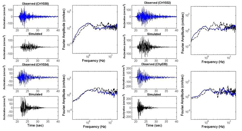
Civil Engineering and Architecture 9(4): 1217-1227, 2021 1219
The f c and f max in equation 8 are the corner frequency
G max = sup {G (ω )} (4)
ω and the high cut-off frequency respectively. In this paper,
we use the relationship between rise time and corner
where G (ω ) is the Fourier transform of G (t ) .
frequency [25] to calculate the f c .
2.2. Source Inversion f c ≈ 0. 6 (9)
σk
The apparent source time functions, which calculated
It is a brand-new attempt to figure out the f c by
by the hybrid blind deconvolution method retrieved from
different stations, describe the moment release watched considering the f c as variable on the fault plane. There is a
just at different distances and orientations to the different formula to calculate f c , however, the method
earthquake [20]. From above viewpoint, we applied the considered f c as a constant value on the fault plane [26].
method in Baumont and Courboulex [21] to invert the
P ( f , f max ) is a high frequency cut-off filter and it has the
kinematic rupture process of the earthquake. The ASTF is
modeled as a time series of Gaussians by Baumont and form of the fourth-order Butterworth filter. It is expressed
Courboulex [21], as the following
−1
f 8
t −Tk −Tpk 2
µ Ak −0.5 ( −2 )2
ASTF (t ) =
2π
∑σ e σk
dxdy (5) P( f , f max ) = 1 + (10)
k k f max
where Tp is the travel time delay between the sub-fault k,
k For the generation of a random time series with the
and the nucleation point to the station, µ is rigidity, dx characteristics of a typical strong motion, the duration of
and dy are sub-fault dimension. Based on the IASPEI 91 the ground motion Td is defined
model (Kennett and Engdahl [22]) the apparent velocities Td = Ts + T p (11)
were calculated and then Tp were calculated by the k
apparent velocities. In order to optimize the non-linear Ts is the rise time and Tp is the path duration
inversion of ASFTs, we employ GA algorithm to invert depending on the epicentral distance empirical relation
the distributions of ( Ak , Tk , σ k ) on the fault. [27]. An envelope function w(t ) of accelergram is given
for a more realistic shape of the acceleration time series.
2.3. Stochastic Method The envelope function of Saragoni and Hart [28] is used
and defined as follow
The radiated seismic energy in the form of elastic wave
w(t ) = at b e − ct H (t ) (12)
has general spectral characteristics at a specific site.
Considering the shear wave contribution to the strong where
motion, the acceleration spectrum A( f ) of shear wave at
e
a distance r from a fault with seismic moment M 0 is a = ( Td ) b (13)
ξ
defined as [17,23]
− ξ ln(η ) (14)
A( f ) = CM 0 S ( f , f c ) P( f , f max )e
( −πfr / Qβ )
(6) b=
r 1 + ξ {ln(ξ ) − 1
Rθφ ⋅ FS ⋅ PRTITN (7) b (15)
C= c= Td
4πρβ 3 ξ
where Rθφ is the radiation pattern, FS the free surface ξ and η are both of constants and H (t ) is the unit-step
amplification effects, PRTITN is a constant, ρ and β function.
are the density and the shear wave velocity. The anelastic
attenuation Q value is represented by a mean
frequency-dependent quality factor for the surrounding 3. Results
area. The source spectrum S ( f , f c ) is defined as ω −2
3.1. Apparent Source Time Function
model (Brune [24])
(2πf ) 2 (8) In order to determine the direction of the rupture, we
S ( f , fc ) = choose 10 teleseismic stations (Figure 1) uniformly
f
1 + ( c )2
f max distributed around the epicenter of the Chia-Yi
earthquake.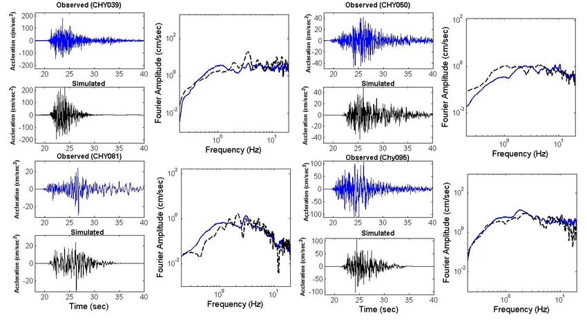
1220                         The Kinematic Source Process of the MW 5.9, 1999 Chia-Yi Taiwan Earthquake
                                 from Teleseismic Data Using the Hybrid Blind Deconvolution Method

                                                                            on the fault. In other words, an observed STF or an STF
                                                                            retrieved from a specific station only describes the
                                                                            moment release watched just at that distance and
                                                                            orientation to the earthquake [20]. Based on the above
                                                                            viewpoint, we can derive the rupture process and rupture
                                                                            direction from the ASTFs. In the Figure 4, it can be seen
                                                                            that the shapes and amplitudes of the apparent source time
                                                                            functions are variable with the different azimuth angles.
                                                                            The distinctive differences among the shapes and
                                                                            amplitudes of the ASTFs allow us to take conclusions
                                                                            with respect to the emergence of directivity effects. The
                                                                            ASTFs obtained at different stations are composed of at
                                                                            least two major sub-events; it is reasonable to conclude,
                                                                            therefore, that this earthquake was a complicated event. It
                                                                            is trivial that the simple Brune model in seismology is not
                                                                            suitable to explain the complex rupture behaviors of this
                                                                            Chia-Yi earthquake.

Figure 1. Location of the epicenter (star) and the far-field ten stations
used (triangles) for the earthquake in Chia-Yi, Taiwan.

   The focal mechanism of the Chia-Yi earthquake is
shown in Figure 2. Figure 3 shows the broadband P-wave
displacement recordings of the vertical components of the
stations. The apparent source time functions estimated by
using the hybrid blind deconvolution method (real line)
                                                                            Figure 2. (a) Fault plane solution of the October 22, 1999 Chia-Yi
are shown in Figure 4. Taking account into the physical                     earthquake in Taiwan. The parameters of Plane 1 are strike 460, dip 560
characteristics of an STF, an STF is the function that                      and rake 1250. The parameters of Plane 2 are strike 1770, dip 500 and
describes the time history of the seismic moment released                   rake 540. (b) 3-D stereo of the fault plane solution.

                           Figure 3. P-wave displacement recordings (vertical component) at the ten broadband stations.
Civil Engineering and Architecture 9(4): 1217-1227, 2021                                             1221

Figure 4. Comparison of the ASTFs, as calculated by the hybrid blind deconvolution method (solid lines) and the synthetic ASTFs (dashed lines) using
the inverted kinematic source model.

Figure 5. Relationship between the pulse widths of the durations of the ASTFs and the azimuths of the stations studied by using the least-squares
                                                                                                    。
method. Based on the regression curve, the rupture direction is toward the west-northwest (about 324 ).

  For a source viewed from a large distance, the ASTF                      epicenter; and φ0 is the direction of the propagation of
duration τ changes with the azimuth and can be                             the rupture. The relationships between pulse widths
expressed as (Nakanishi [29]):                                             durations of the ASTFs and the azimuths of the stations
                     τ = τ 0 − k cos(φ − φ0 )                      (16)    can be investigated by employing the least-squares
                                                                           method. The parameters ( τ 0 , φ0 ) is equal to (6.5, 324.3)
where τ 0 is the non-azimuthal source duration; k is a                     and the results are shown in Figure 5. If the rupture
constant; φ is the azimuth of the station viewed from the                  velocity were assumed 3km/s, the dimension of the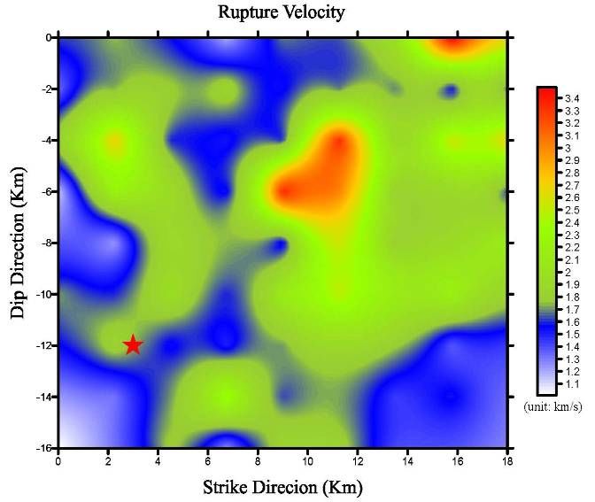
1222                    The Kinematic Source Process of the MW 5.9, 1999 Chia-Yi Taiwan Earthquake
                            from Teleseismic Data Using the Hybrid Blind Deconvolution Method

rupture plane can be estimated approximately 18km at
least. It indicates that the azimuth of the rupture is about
324o , which suggests that the rupture propagated in the
northwest direction. The direction of slip vector of plane 1,
one of the focal planes of the earthquake (Figure 2) agrees
with the retrieved result from our study. It follows that
plane 1 can justifiably be recognized as the real fault plane.
The east dipping slip model is though as the preferred
model. It is well consistent with the result of strong
motion inversion in reference [1].

3.2. Source Model

   With the ASTFs of 10 stations, we can invert the
distributions of ( Ak , Tk , σ k ) along the fault by GA
algorithm to optimize the non-linear inversion of the            Figure 6. Image of the slip distribution on the thrust fault of Chia-Yi
ASFTs. We fix the dimensions of the fault at about 18km          earthquake, as derived from source inversion. The star represents the
                                                                 location of the hypocenter.
× 16km with the epicenter located at the depth of 16km.
The fault is divided into equal area 2km × 2 km sub-faults.
Figure 6 shows the distribution of the slip amplitudes on
the fault. The slip amplitudes range from 0.004m to 2.2m,
and their average is about 0.38m. In general, the slip
appears to be concentrated in two patches. One of the
patches located at about 2 km of the right lower part from
the nucleation point, the other located the left upper corner
on the fault. Figure 7 displays the distribution of the
rupture velocities on the fault. It is worth noting that the
region with the higher value of 3.5 km/s is located at
about 8-12 km in strike direction of the fault. In this
region, it had higher rupture velocities and lower slip
amplitudes; therefore, it means that the fault in this region
could be relatively weak. It may be attributed to the
weakness of low-density rocks in the zone (Ozacar et al.,
[30]) or the fluids in this region might have such reduced       Figure 7. Image of the rupture velocities distribution on the thrust fault
friction that tectonic stress was produced by the relatively     of Chia-Yi earthquake, as derived from source inversion. The star
                                                                 represents the location of the hypocenter.
thin, brittle part of the crust (Fisher et al. [31]). The
distribution of rise time on the fault, as determined in the
present study, is shown in Figure 8. The maximum rise
time on the individual sub-fault is about 1.1 sec, which is
about one-sixth of the total rupture duration (6.5 sec) of
the earthquake rupturing process. Comparing distributions
of the slip and rise time, we find that the larger slip
amplitude corresponds to the larger rise time on each
subfault. Figure 9 shows the relationship of the linear
regressions between slip amplitudes and rise time. This
relationship is quite similar to the result of Chi-Chi
earthquake [20]. The comparison of the retrieved ASTFs
calculated by the hybrid blind deconvolution (solid line)
and the synthetic ASTFs (dashed line) using the inverted
kinematic source model is displayed in Figure 2. The
correlation coefficients between the synthetic and               Figure 8. Image of the rise time distribution on the thrust fault of
calculated ASFTs are high and at approximately 0.8~0.98.         Chia-Yi earthquake, as derived from source inversion. The star represents
                                                                 the location of the hypocenter.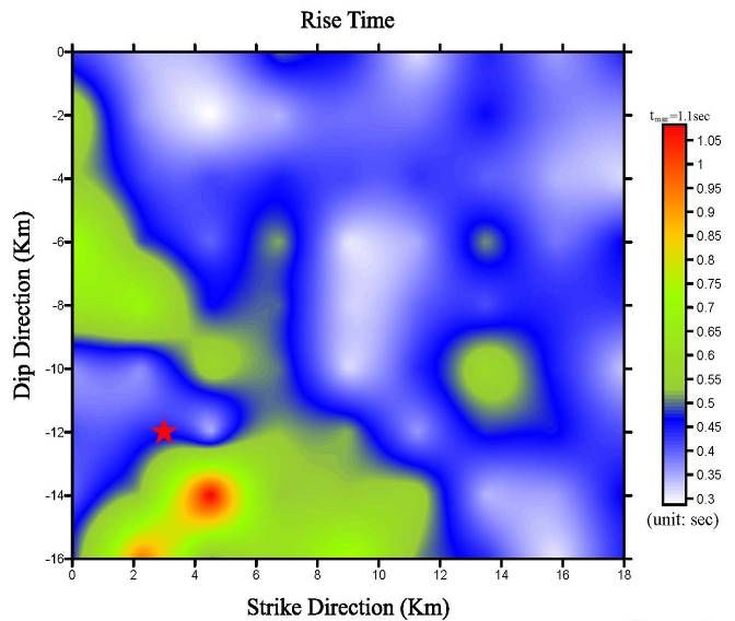
Civil Engineering and Architecture 9(4): 1217-1227, 2021                                                       1223

Figure 9. Relationship between the slip amplitude and rise time of the slip functions. The larger slip amplitudes have a longer rise time on the
sub-faults.

3.3. Stochastic Simulation                                               Joyner [33]) in the present study. The goal of this study is
                                                                         to investigate the source effects on the frequency and time
   For identifying the validation of the inverted source                 domain of the seismic signals; therefore, we assume the
model, we use the stochastic method to simulate the                      path and the local site effects appear as the simplest
strong ground motions near the epicenter. There are 12                   forms.
vertical component accelerograms of different stations
simulated. The distribution of 12 stations is shown in                   Table 1. Modeling parameters used to stochastically simulate strong
                                                                         ground motion from the 1022 Chia-Yi earthquake.
Figure 10. The 12 stations at epicentral distances range
from 3.28 to 29 km. In above simulation, we assume that                          Parameter                         Parameter Value
the stations are all installed on the rock to detect the                     Fault orientation                    Strike 460, dip 560
source effect on the ground motions near the epicenter.                       Fault dimension               Length 18km, Width 16km
The complexity of the faulting process largely dominates
                                                                              Magnitude (ML)                                  6.4
the character of the signal at near source distances, when
the site effects can be considered as weak or negligible                    Number of subfaults                               9×8
(Emolo and Zollo [32]). The modeling parameters for the                            Q( f )                Q( f ) = 150 f 0.2 , f ≤ 20 Hz
application of the simulated method are listed in Table 1.                 Geometric spreading                                1/R
The material properties are described by density, ρ , and                       kappa (sec)                               0.006
shear-wave velocity, β , which are given the values
                                                                           Windowing function                       Saragoni-Hart
2.8g/cm3 and 3.7km/sec, respectively. We applied a
geometric spreading operator 1 R , and the anelastic                          Crustal density                           2.8g/cm3
attenuation was represented as Q( f ) = 150 f 0.2 , f ≤ 20 Hz               Shear-wave velocity                        3.7km/sec
derived from strong motion in southwest Taiwan. The                                                     Td = Ts + Tp , Ts is rise time
effect of the near-surface attenuation was employed by the                   Distance-depend
factor exp(−πκf ) [23]. The kappa operator, κ , was given                     duration (sec)                         0 ,            R < 10km
                                                                                                     Tp =
the value 0.006 sec for very hard-rock site (Boore and                                                      0.16 ( R − 10),         10km ≤ R < 70km.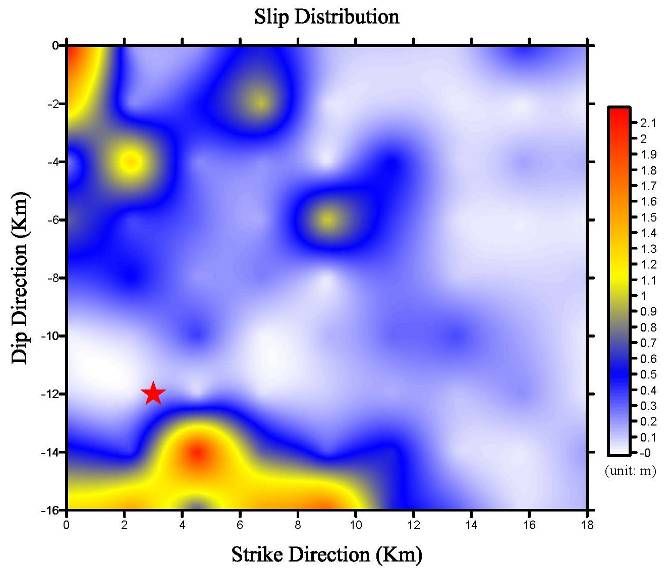
1224                        The Kinematic Source Process of the MW 5.9, 1999 Chia-Yi Taiwan Earthquake
                                from Teleseismic Data Using the Hybrid Blind Deconvolution Method

   In Figure 11~13 we present the results of the stochastic               may be attributed to inadequacies in the representation of
simulations and their comparisons with the observed                       the path or the local site.
strong ground-motion recordings. Peak ground
acceleration are well reproduced, expect the stations
CHY030 and CHY034. CHY030 is under-estimated about
a factor of 0.75 and CHY030 is over-estimated about a
factor about 1.45. The amplitudes of the observed spectra
of the stations (CHY009, CHY034, CHY038, CHY039,
CHY095) which the epicenters are less than 13km are
generally matched well with the observed, especially the
station CHY009. It demonstrates that the inverted source
model is quite reliable in this study. The phenomenon
may be due to the fact that the seismic signal of the station
near the epicenter is so largely affected by the source that
the other effects of path and site are not crucial.
Nevertheless, large discrepancies exist in the lower
frequency at some stations (CHY028, CHY029, CHY032,
CHY050 and CHY081). The epicentral distances of these                     Figure 10. The locations of 12 strong motions stations (triangles) and
stations are ranging from 15km to 28.24km, depending on                   the epicenter (star) of the earthquake occurred on October 22, 1999,
the source-station distance. The reasons for this misfit                  Chia-Yi, Taiwan.

Figure 11. The comparisons of the observed recordings and simulated waveforms, and the comparisons of Fourier spectras of observed and simulated.
The stations shown here are CHY009, CHY014, CHY028 and CHY029.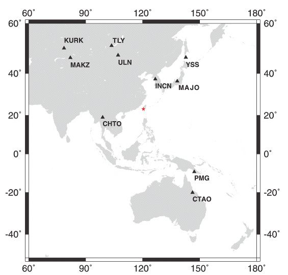
Civil Engineering and Architecture 9(4): 1217-1227, 2021                                           1225

Figure 12. The comparisons of the observed recordings and simulated waveforms, and the comparisons of Fourier spectras of observed and simulated.
The stations shown here are CHY030, CHY032, CHY034 and CHY038.

Figure 13. The comparisons of the observed recordings and simulated waveforms, and the comparisons of Fourier spectras of observed and simulated.
The stations shown here are CHY039, CHY050, CHY081 and CHY095.

4. Conclusions                                                            mechanism. The slip distribution on the fault plane
                                                                          concentrates on two patches. From the higher rupture
   We apply the hybrid blind deocnvolution method to                      velocity with the lower slip amplitude, the relative weak
derive the temporal-spatial rupture process of the ML 6.4                 region is found on 8-12 km in strike direction of the fault.
earthquake which occurred on the Chia-Yi, Taiwan, on                      For the most part, the larger slip amplitudes correspond to
October 22, 1999. In this study, the total rupture duration               larger rise times on the subfaults.
of the main shock is about 6.5 sec. Based on the                             The stochastic method is employed to confirm the
relationship between the pulse widths of the ASFTs and                    reliability of the inverted source model. The result shows
the azimuths of the stations, we can distinguish the                      that the comparison between simulated and observed of
ruptured plane (SE-NW direction) from the focal                           the signal in the station near the epicenter is quite matched.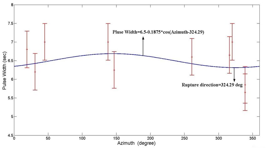
1226                       The Kinematic Source Process of the MW 5.9, 1999 Chia-Yi Taiwan Earthquake
                               from Teleseismic Data Using the Hybrid Blind Deconvolution Method

It reveals the precision of the source model and the source               seismiological data, Geophys. Res. Lett., 29(15), 1638, doi:
effect dominates the seismic signal near the epicenter. The               10.1029/ 2001GL014261, 2002.
effects of path and site are weighting in the signals of the         [13] I. A. Beresnev and G. M. Atkinson. Modeling finite-fault
                                                                          radiation from the ω spectrum, Bull. Seism. Soc. Am., 87,
                                                                                              n
stations with the epicentral distances increasing. The next
steps are applied these simulations to the earthquake                     67-84, 1997.
disaster preventions and the field in earthquake                     [14] N. Lam, J. Wilson and G. Hutchinson. Generation of
engineering. There, the results in the paper are playing a                synthetic earthquake accelerograms using seismological
crucial role in actual applications.                                      modeling: a review, Journal of Earthquake Engineering,
                                                                          4(3), 321-354, 2000.
                                                                     [15] S. Suzuki and K. Asano. Simulation of near source ground
                                                                          motion and its characteristics, Soil Dyn. and Earthq. Engng,
                                                                          20, 125-136, 2000.
REFERENCES
                                                                     [16] R. R. Castro , A. Rovelli, M. Cocco, M. D. Bona and F.
[1]    W. C. Chi and D. Dreger. Crustal deformation in Taiwan:            Pacor . Stochastic simulation of strong-motion records from
       Results from finite source inversions of six Mw>5.8 Chi-Chi        the 26 September 1997 (Mw 6), Umbria-Marche (Central
       aftershocks, J. Geophys. Res., 109, B07305, doi:                   Italy) earthquake, Bull. Seism. Soc. Am., 91, 27-39, 2001.
       10.1029/2003JB002606, 2004.
                                                                     [17] D. M. Boore. Stochastic simulation of high-frequency
[2]    M. W. Huang, J. H. Wang, R. D. Hwang and K. C. Chen.               ground motions based on seismological models of the
       Estimates of source parameters of two large aftershocks of         radiated spectra, Bull. Seism. Soc. Am., 73, 1865-1894,
       the 1999 Chi-Chi, Taiwan, earthquake in the Chia-Yi area,          1983.
       TAO, 13(3), 299-312, 2002.
                                                                     [18] Z. Roumelioti, A. Kiratzi and N. Theodulidis. Stochastic
[3]    H. Luo and Y. Li. The application of blind channel                 strong ground-motion simulation of the 7 September 1999
       identification technique to prestack seismic deconvolution,        Athens (Greece) earthquake, Bull. Seism. Soc. Am., 94,
       Proceedings of the IEEE, 86, No. 10, 2082-2088, 1998.              1036-1052, 2004.
[4]    D.R. Velis and T.J. Ulrych. Simulated annealing wavelet       [19] M. Bertero, D. Bindi, P. Boccacci, M. Cattaneo, C. Eva and
       estimation via fourth-order cumulant matching, Geophysics          V. Lanza. A novel blind-deconvolution method with an
       61, 1939-1948, 1996.                                               application to seismology, Inverse Problem, 14, 815-833,
                                                                          1998.
[5]    I. Santamaria, C. J. Pantaleon, J. Ibanez, and A. Artes.
       Deconvolution of seismic data using adaptive Gaussian         [20] L. S. Xu, Y. T. Chen, T. L. Teng and G. Patau.
       mixtures, IEEE Trans. on Geosciences and Remote Sensing,           Temporal-Spatial Rupture Process of the 1999 Chi-Chi
       37, 855-859, 1999.                                                 Earthquake from IRIS and GEOSCOPE Long-Period
                                                                          Waveform Data Using Aftershocks as Empirical Green’s
[6]    A. Zerva, A. Petropulu and P. Y. Bard. Blind deconvolution         Functions, Bull. Seism. Soc. Am. 92, 3210-3228, 2002.
       methodology for site response evaluation exclusively from
       ground surface seismic recordings, Soil Dyn. and              [21] D. Baumont and F. Courboulex. Slip distribution of the Mw
       Earthq. Engng, 18, 47-57, 1999.                                    5.9, 1999 Athens earthquake inverted from regional
                                                                          seismiological data, Geophys. Res. Lett., 29(15), 1638, doi:
[7]    L. A. Pflug. Principal domains of the trispectrum signal           10.1029/ 2001GL014261, 2002.
       bandwidth, and implications for deconvolution, Geophysics,
       65, No.3, 958-969, 2000.                                      [22] B. L. N. Kennett and E. R. Engdahl. Travel times for global
                                                                          earthquake location and phase identification, Geophys. J.
[8]    B. Y. Liao and H. C. Huang. A refinement of the                    Int., 105, 429-465, 1991.
       generalized blind deconvolution method based on the
       Gaussian mixture and its application, TAO, 14(3), 1-11,       [23] G. M. Atkinson and D. M. Boore. Some comparisons
       2003.                                                              between recent ground-motion relations, Seism. Res. Lett.,
                                                                          68, 24-40, 1997.
[9]    B. Y. Liao and H. C. Huang. Estimation of the source time
       function based on blind deconvolution with Gaussian           [24] J. Brune. Tectonic stress and the spectra of seismic shear
       Mixtures, Pure and Applied Geophys., 162, 479-494, 2005.           waves from earthquakes, J. Geophys. Res., 75, 4997-5009,
                                                                          1970.
[10] B. Y. Liao and H. C. Huang. Rupture process of the 2002
     Denali earthquake, Alaska (Mw=7.9) using the                    [25] I. A. Beresnev. Source parameters observable from the
     newly-devised hybrid blind deconvolution, Bulletin of                corner frequency of earthquake spectra, Bull. Seism. Soc.
     Seismological Society of America 98, 162-179, 2008.                  Am., 92, 2047-2048, 2002.
[11] B. Y. Liao, Y. T. Yeh, T. W. Sheu, H. C. Huang and L. S.        [26] Z. Roumelioti and A. Kiratzi. Stochastic simulation of
     Yang. A Rupture Model for the 1999 Chi-Chi Earthquake                strong-motion records from the 15 April 1979 (M 7.1)
     from Inversion of Teleseismic Data Using the Hybrid                  Montenegro earthquake, Bull. Seism. Soc. Am., 92,
     Homomorphic Deconvolution Method, Pure and Applied                   1095-1101, 2002.
     Geophysics, 170 (3), 391-407, 2013.
                                                                     [27] G. M. Atkinson and D. M. Boore. Evaluation of models for
[12] D. Baumont and F. Courboulex. Slip distribution of the Mw            earthquake source spectra in Eastern North America, Bull.
     5.9, 1999 Athens earthquake inverted from regional                   Seism. Soc. Am., 88, 917-934, 1998.
Civil Engineering and Architecture 9(4): 1217-1227, 2021 1227
[28] G. R. Saragoni and G. C. Hart. Simulation of Artificial [31] M. A. Fisher, W. J. Nokleberg, N. A. Ratchkovski, L.
Earthquakes, Earthquake Engineering and Engineering Pellerin, T. M. Brocher and J. Booker. Geophysical
Vibration, 4(1), 1-10, 1974. investigation of the Denali fault and Alaska range orogen
within the aftershock zone of the October-November 2002,
[29] I. Nakanishi. Source process of the 1989 Sanriku-Oki M=7.9 Denali fault earthquake, Geology, 32, 269-272, doi:
earthquake, Japan: source function determined using 10.1130/G20127.1, 2004.
empirical Green’s function, J. Phys. Earth., 39, 661-667,
1991. [32] A. Emolo and A. Zollo. Accelerometric radiation
simulation for the September 26, 1997 Umbria-Marche
[30] A. A. Ozacar, S. L. Beck and D. H. Christensen. Source (Central Italy) main shocks, ANNALI DI GEOFISICA,
process of the 3 November, 2002 Denali fault earthquake 44(3), 605-617, 2001.
(central Alaska) from teleseismic observations, Geophys.
Res. Lett., 30(12), 1638, doi: 10.1029/ 2003GL017272, [33] D. M. Boore, and W. B. Joyner. Site amplifications for
2003. generic rock sites, Bull. Seism. Soc. Am., 87, 327-341, 1997.You can also read