The Limit Order Book Recreation Model (LOBRM): An Extended Analysis
←
→
Page content transcription
If your browser does not render page correctly, please read the page content below
The Limit Order Book Recreation Model
                                                     (LOBRM): An Extended Analysis

                                                            1[0000−0001−7823−8527]
                                               Zijian Shi                            and John Cartlidge1[0000−0002−3143−6355]

                                                Department of Computer Science, University of Bristol, Bristol BS8 1UB, UK
                                                              {zijian.shi,john.cartlidge}@bristol.ac.uk
arXiv:2107.00534v1 [q-fin.TR] 1 Jul 2021

                                                   Abstract. The limit order book (LOB) depicts the fine-grained demand
                                                   and supply relationship for financial assets and is widely used in mar-
                                                   ket microstructure studies. Nevertheless, the availability and high cost
                                                   of LOB data restrict its wider application. The LOB recreation model
                                                   (LOBRM) was recently proposed to bridge this gap by synthesizing the
                                                   LOB from trades and quotes (TAQ) data. However, in the original LO-
                                                   BRM study, there were two limitations: (1) experiments were conducted
                                                   on a relatively small dataset containing only one day of LOB data; and
                                                   (2) the training and testing were performed in a non-chronological fash-
                                                   ion, which essentially re-frames the task as interpolation and potentially
                                                   introduces lookahead bias. In this study, we extend the research on LO-
                                                   BRM and further validate its use in real-world application scenarios. We
                                                   first advance the workflow of LOBRM by (1) adding a time-weighted
                                                   z-score standardization for the LOB and (2) substituting the ordinary
                                                   differential equation kernel with an exponential decay kernel to lower
                                                   computation complexity. Experiments are conducted on the extended
                                                   LOBSTER dataset in a chronological fashion, as it would be used in
                                                   a real-world application. We find that (1) LOBRM with decay kernel
                                                   is superior to traditional non-linear models, and module ensembling is
                                                   effective; (2) prediction accuracy is negatively related to the volatility
                                                   of order volumes resting in the LOB; (3) the proposed sparse encoding
                                                   method for TAQ exhibits good generalization ability and can facilitate
                                                   manifold tasks; and (4) the influence of stochastic drift on prediction
                                                   accuracy can be alleviated by increasing historical samples.

                                                   Keywords: Limit order book · Time series prediction · Financial ma-
                                                   chine learning.

                                           1     Introduction

                                           The majority of financial exchange venues utilise a continuous double auction
                                           (CDA) mechanism [11] for matching orders. Under CDA formation, both ask
                                           orders (orders to sell a given quantity at a given price) and bid orders (orders to
                                           buy a given quantity at a given price) arrive at the venue continuously, with no
                                               This is a preprint manuscript accepted for publication at ECML-PKDD 2021.
2       Z. Shi and J. Cartlidge

minimum time interval limit. When a new order arrives, if it does not immedi-
ately execute, it will enter the limit order book (LOB); which contains a list of
current bids and a list of current asks, both sorted by price-time priority. There-
fore, the LOB contains valuable information on the instantaneous demand and
supply for a particular financial asset (e.g., a stock, a commodity, a derivative,
etc.). For this reason, LOB data has been used for many and various studies,
including exploration of the price formation mechanism [20], market anomaly
detection [26], and testing of trading algorithms [1].
    However, there remain some obstacles for the wider application of LOB data.
Firstly, LOB data subscription fees are usually high, sometimes amounting to
tens of thousands of dollars per annum.1 This might be a trivial sum for an
institutional subscriber, however for individual investors and researchers this
significant expense can hold them back. Further, LOB data is entirely unavailable
in venues that deliberately do not make order information public, for instance
some e-commercial markets and dark pools (e.g., see [6,7]). This challenge attracts
researchers to consider the possibility of recreating the LOB from a more easily
available source, such as trades and quotes (TAQ) data. TAQ data contains the
top price level information of a LOB (the lowest-priced ask and highest-priced
bid), together with a history of transactions. It is published to the public for
free in most venues. Blanchet et al. [5] have previously demonstrated that it is
possible to predict daily average order volumes resting at different price levels of
the LOB, using only TAQ data for parameter estimation. More recently, from a
deep learning perspective, the LOB recreation model (LOBRM) was proposed
to formalize the task as a time series prediction problem, and an ensembled
recurrent neural network (RNN) model was successfully used to predict order
volumes in a high frequency manner for the first time [23]. Nevertheless, there
exist two key restrictions in the LOBRM study: (1) The original LOBRM study
was conducted in an interpolation style on only one day’s length of LOB data, for
two stocks. For the model to be applied in a real world application scenario, such
as online prediction of market price movements, LOBRM performance requires
evaluation on an extended multi-day dataset, with chronological training and
testing such that there is no possibility of lookahead bias; (2) The ordinary
differential equation (ODE) kernel used in the original LOBRM model has high
computation complexity and is therefore inefficient for more realistic application
scenarios when large amounts (weeks or months) of training data is used.

Contributions:
 1. We advance the workflow and structure of the LOBRM model, such that: (i)
    a time-weighted z-score standardization for LOB features is used to enhance
    the model’s generalization ability; and (ii) the original ODE kernel is sub-
    stituted for an exponential decay kernel to enable faster inference of latent
    states, greater runtime efficiency, and a reduction in overfitting.
 2. We use chronological training and testing to conduct experiments on an
    extended LOBSTER dataset that is an order of magnitude larger than the
1
    http://www.nasdaqtrader.com/Trader.aspx?id=DPUSdata
Exploring the LOB Recreation Model                                    3

              BID                ASK                         BID               ASK               BID                    ASK
        Qty     Price    Price         Qty             Qty     Price   Price         Qty   Qty     Price        Price         Qty
        10      $50      $56        20                 10    $50       $57        10       10      $52          $57        10
        20      $49      $57        10      20 units   20    $49       $60        40       10      $50          $60        40
        50      $48      $60        40      bought     50    $48       $62       100       20      $49          $62       100
                                             at $56
       100      $45      $62       100                100    $45       $63        20       50      $48          $63        20
      Market events T1           Limit bid order submission:    T2       Limit bid order submission:       T3
         stream                          20 units at $56                        10 units at $52

Fig. 1. A LOB of four price levels evolving with time. White and blue boxes indicate
the top level and deeper levels of the LOB. Grey boxes indicate market events stream.
Orange box indicates trade records. White and orange boxes together form TAQ.

    original dataset. We find that: (i) LOBRM with continuous decay kernel
    is superior in modelling the irregularly sampled LOB; and (ii) the module
    ensembling of LOBRM is effective.
 3. We draw new empirical findings that further enrich the current literature: (i)
    the proposed sparse encoding method for TAQ data has good generalization
    ability and can facilitate manifold tasks including LOB prediction and price
    trend prediction; (ii) prediction accuracy of the LOBRM is negatively related
    to volume volatility at unseen price levels; and (iii) the influence of stochastic
    drift on model performance can be alleviated by increasing the amount of
    historical training samples.

2     Background and Related Work

2.1   The Limit Order Book (LOB)
In a CDA market, bids and asks with specified price and quantity (or volume)
are submitted, cancelled, and transacted continuously. The LOB contains an
ask side and a bid side, with ask orders arranged in price ascending order and
bid orders arranged in price descending order. Ask orders with the lowest price
(best ask) and bid orders with the highest price (best bid) form the top level of a
LOB, and their respective prices are called quotes. If a newly submitted ask (or
bid) price is not higher (or lower) than the best bid (or ask), a trade happens.
TAQ data contains all historical quotes and trades in the venue. That is, LOB
data contains strictly more information than TAQ data. Fig. 1 provides a visual
illustration of a LOB and the relationship between the LOB and the TAQ data.
    Traditional statistical models of the LOB assume that LOB evolution follows
the rules of a Markovian system, with market events (order submission, cancel-
lation, and transaction) following stochastic point processes, such as a Hawkes
process or a Poisson process [2,10]. This formulation generalizes a LOB mar-
ket of high complexity to a dynamic system controlled by a few parameters,
where probabilistic theorems like the law of large numbers [12] and stationary
equilibrium in a Markovian system [5] can be utilized to draw long-term em-
pirical conclusions. However, while statistical modelling can capture long term
4 Z. Shi and J. Cartlidge
behaviour patterns of the LOB, these models cannot consistently perform well
in a high frequency domain. In recent years, there has been an emergence of re-
search using deep learning approaches to model and exploit the LOB. Sirignano
et al. [24] performed a significant study on a comprehensive pool of 500 stocks.
They revealed that features learned by a Long Short-Term Memory (LSTM) net-
work can be utilized to predict next mid-price movement direction {up, down}
with accuracy range [0.65, 0.76] across all 500 stocks. Their study also demon-
strated that deep learning models suffer less from problems such as stochastic
drift that exist in statistical models of the LOB. Other deep learning studies of
the LOB include extracting high frequency indicators [21,25], predicting future
stock price movement [16,27], and training reinforcement trading agents [13,18].
2.2 Generating Synthetic LOB Data
Synthetic LOB data, generated by models that learn from the real LOB or
imitate the stylized facts of a CDA market, has been used as an alternative when
real LOB data is unavailable. The advantages of using synthetic LOB data lie
in its low cost and infinite availability. It has been widely adopted to backtest
trading algorithms, explore market dynamics, and facilitate teaching activities.
Synthetic LOB data can be generated using three mainstream methodolo-
gies. Agent-based models have been well studied and are the most popular
approach for generating a synthetic LOB. By configuring agents that trade us-
ing common strategies, such as market makers, momentum traders, and mean
reversion traders, the synthetic LOB can closely approximate the stylised facts
of a real LOB [17]. Stock market simulators have a long history, from the Santa
Fe artificial stock exchange [3] to recent multi-agent exchange environments [4].
Generative models attempt to learn regularities embedded in market event
streams or the LOB directly. One representative research by Li et al. [15] utilized
generative adversarial networks to learn and replicate the historical dependency
among orders. The synthesised order stream and resulting LOB were found to
closely resemble the real market data.
We consider the aforementioned two approaches as unsupervised, since no real
LOB data is used to verify the authenticity of the generated data. Model quality
can only be verified by testing whether certain stylized facts exist in the synthetic
data. In contrast, supervised models use real LOB data as ground truth. As
indicated in [5], TAQ data is informative of LOB volumes for small-tick stocks.
By modelling the tail probability of price change per trade in a Markovian LOB,
daily average order volumes at unseen price levels can be estimated by the steady-
state distribution of the infinite server queue. Shi et al. [23] further formulate
the task of generating a synthetic LOB as a time series prediction problem using
a continuous RNN. The proposed model (LOBRM) is able to predict LOB order
volumes using a defined length of TAQ data as input. As long as a historical
TAQ trajectory is available, the model is able to produce a historical replay of
the LOB based on the knowledge it learned from supervised training. This paper
concentrates on a further exploration of the LOBRM model presented in [23].Exploring the LOB Recreation Model 5
3 Model Formulation
3.1 Motivation
The LOBRM model represents the first attempt to synthesize LOB data from
a supervised deep learning perspective [23]. LOBRM is essentially an ensemble
of RNNs that take TAQ data as input and produce LOB volume predictions as
output. However, in the original study, there were three restrictions present: (1)
Experiments were performed using a relatively small LOB dataset consisting of
only one day’s LOB data for two small-tick stocks. To verify its generalization
ability, LOBRM requires testing on multi-day LOB data for a variety of stocks.
(2) Experiments adopted a non-chronological approach to the formation of time
series samples, such that samples were shuffled before splitting into training and
testing sets. We intend to test model performance using a strictly chronological
approach to ensure that LOBRM is applicable to real world online scenarios,
with no possibility of introducing lookahead bias. Specifically, we use the first
three days’ data for training, the fourth day’s data for validation, and the fifth
day’s data for testing. Time series samples are not shuffled, thus ensuring that
chronological ordering is preserved. (3) The core module of the original LOBRM
made use of an ODE-RNN, a RNN variant with ODE kernels to derive fine-
grained time-continuous latent states [22]. As the computational complexity of
ODE-RNN is n times that of a vanilla RNN – where n is the granularity of
the latent state – it is not efficient for training data of large size. Therefore, we
substitute the ODE-RNN for an RNN-decay module [8], which has been shown
to be a more time-efficient model for irregularly sampled time series [14].
3.2 Problem Description
To simplify the problem of recreating the LOB, we make the same assumptions
proposed in [23]: (1) Following common practice (e.g., [5,12]), the bid and ask
sides of the LOB are modelled separately; (2) We only consider instantaneous
LOB data at the time of each trade event, and ignore the LOB for all other
events, such as order submission and cancellation; (3) We only consider the top
five price levels of the LOB; (4) We assume that the price interval between each
price level is exactly one tick – the smallest increment permitted in quoting
or trading a security at a particular exchange venue – which is supported by
empirical evidence that orders in the LOB for small-tick stocks tend to be densely
distributed around the top price levels [5]. Following these assumptions, the price
at different LOB levels can be directly deduced from the known quote price at
target time. Therefore, the LOB recreation task resolves to the simpler problem
of only predicting order volumes resting at each price level.
For generalization, we denote trades and quotes streams as {T Di }i∈n and
{QTi }i∈n respectively, and trajectories of time points for TAQ records as {Ti }i∈n
indexed by n = {1, . . . , N }, where N equals the number of time points in TAQ.
The LOB sampled
at {Ti }i∈n are
denoted as {LOBi }i∈n . For each record at time
a(1) a(1) b(1) b(1) a(1) a(1) b(1) b(1)
Ti , QTi = pi , vi , pi , vi , where pi , vi , pi , vi denote best ask6 Z. Shi and J. Cartlidge
price, order volume at best ask, best bid price, and order volume at best bid,
respectively. T Di = ptd td td td td td
i , vi , di , where pi , vi , di denote price, volume, and
direction of the trade, with +1 and −1 indicating orders being sold or bought.
a(l) a(l) b(l) b(l)
LOBi = (pi , vi , pi , vi ) depicts the price and volume information at all
price levels, with l ∈ (1, ..., L), here L = 5. From the aforementioned model
a(l) a(1) b(l) b(1)
assumptions, we have pi = pi + (l − 1)τ and pi = pi − (l − 1)τ , where τ
is the minimum tick size (1 cent in the US market). For a single sample, the model
a(2) a(L) b(2) b(L)
predicts (vI , ..., vI ) and (vI , ..., vI ) conditioned on the observations of
{QTi }I−S:I and {T Di }I−S:I , with S being the time series sample size, i.e., the
maximum number of time steps that the model looks back in TAQ data history.
3.3 Formalized Workflow of LOBRM
LOB Data Standardization As we intend to apply the LOBRM model on
LOBs of five days’ length for different financial assets, data standardization is
necessary for the model’s understanding of data of various numerical scales. We
perform time-weighted z-score standardization on all LOB volumes, based on the
fact that the LOB is a continuous
n o dynamic system with uneven time intervals
(l)
between updates. We use vn and {Tn }0:N to indicate volume trajectory
0:N
on price level l, and affiliated timestamps N as the total number of LOB updates
for training. Time-weighted mean and standard deviation are calculated as:
P N −1 (l)
Mean(l) = i=0 (Ti+1 − Ti ) vi / (TN − T0 ) (1)
2 21
P N −1 (l)
Std(l) = i=0 (Ti+1 − Ti ) vi − Mean(l) / (TN − T0 ) (2)
From empirical
n oobservation, we witness that the volume statistics on deeper
(2−5)
price levels vn have similar patterns, while those statistics deviate from
0:N n o
(1)
volume statistics on the top price level vn . In particular, the top level
0:N
tends to have much lower mean and much higher standard deviation (e.g., see
later Table 1). Thus, we treat ‘top’ and ‘deeper’ levels as two separate sets to
standardize. As trade volumes {vntq }0:N are discrete events and do not persist in
time, we use a normal z-score standardization for trade data. To avoid lookahead
bias, statistics are calculated without considering test data. Finally, using these
statistics, LOBs for training, validation, and testing are standardized.
Sparse Encoding for TAQ TAQ data contains multi-modal information, in-
cluding order type (bid or ask), price, and volume. While under the formulation
of LOBRM, only order volumes at derived price levels (i.e., deeper levels 2-5) are
predicted. We use a one-hot positional encoding, such that only volume infor-
mation is encoded explicitly; while price is indicated by the position of non-zero
elements in the one-hot vector.Exploring the LOB Recreation Model 7
Take the encoding of an ask quote as an example. Conditioned on current
a(1) b(1)
best ask price pI and best bid price pI at TI , we represent the ask quote
a(1) a(1) b(1) b(1)
record (pI−s , vI−s ) and bid quote record (pI−s , vI−s ) at TI−s , s ∈ {0, . . . , S} as:
(
aq a(1)
O2k−1 , where ok+spas = vI−s
bq b(1) (3)
O2k−1 , where ok+spbs = vI−s
a(1) a(1) b(1) b(1)
where k ∈ R, spas = (pI−s − pI )/τ and spbs = (pI−s − pI )/τ . O2k−1 is a
one-hot vector with dimension 1 × (2k − 1); and osp denotes the sp-th element of
the vector. The value of k is chosen to cover more than 90% of past quote price
fluctuations, relative to the current quote price. Here k = 8, which means his-
torical quotes with relative price [−7, +7] ticks are encoded into feature vectors.
Then, a trade record (ptd td td
I−s , vI−s , dI−s ), is represented as:
td td
if dtd
(
O2k−1 , where optd a(1)
−pI
= vI−s I−s < 0
td
I−s
td (4)
O2k−1 , where optd b(1)
−pI
= vI−s if dtd
I−s > 0
I−s
Finally, those three features are concatenated into (Oaq , Obq , Otd ) and are
used as input. It can also be a concatenation of four features, with ask and
bid trade represented separately. Later, in experiment section 4.4, we show this
sparse encoding method can achieve enhanced robustness in LOB volume pre-
diction and price trend prediction.
Market Event Simulator Module (ES) The ES module models the overall
net order arrivals as inhomogeneous poisson processes, and predicts LOB vol-
umes from a dynamic perspective. If an RNN structure is used to iteratively
receive encoded LOB features at every timestep, its latent state can be deemed
as reflective of market microstructure condition over a short historical time win-
dow. A multi-layer perceptron (MLP) layer can then be used to decode latent
states directly into vectors representing net order arrival rates at each price level.
The original LOBRM model uses ODE-RNN, a continuous RNN variant that
learns fine-grained latent state between discrete inputs in a data-driven manner,
to model the continuous evolution of market conditions. In ODE-RNN, a hidden
state h(t) is defined as a solution to an ODE initial value problem. The latent
state between two inputs can then be derived using an ODE solver as:
dh(t)
dt = fθ (h(t), t) where h(t0 ) = h0 (5)
hi 0 = ODEsolver(fθ , hi−1 , (ti−1 , ti )) (6)
in which function fθ is a separate neural network parameterized by θ.
Even though ODE-RNN contributes most to prediction accuracy, it is of
high computation complexity (see Section 3.1). Therefore, for an efficient use of
LOBRM, especially when trained on large amounts of data, or used for online8 Z. Shi and J. Cartlidge
prediction, the ODE-RNN is unsuitable. Also, we find in chronological exper-
iments that the ODE-RNN tends to cause overfitting due to the fully flexible
latent states.
Faced with these challenges, we propose the use of a pre-defined exponential
decay kernel [8,14], instead of the ODE kernel in the ES module. The inference
of latent states between discrete inputs is denoted as:
hi 0 = hi−1 ∗ exp (−fθ (hi−1 ) ∗ Φ (ti−1 , ti )) (7)
hi = GRUunit hi 0 , xi
(8)
where fθ is a separate neural network parameterized by θ, and Φ is a smoothing
function for time intervals to avoid gradient diminishing. A GRU unit [9] is then
used for instant updating of the latent state at input timesteps. The advantages
of employing an exponential decay kernel are threefold: (1) It allows for efficient
inference of latent states; (2) It is a continuous RNN that imitates continuity
of market evolution and includes temporal information within the model struc-
ture itself, sharing the advantages of continuous RNN in modelling irregularly
sampled time series; (3) It is less likely to cause overfitting as the kernel form is
predefined, whereas the latent state evolution in ODE-RNN is fully flexible.
a(2) a(L)
We derive the vector of net order arrival rates ΛI−s = [λI−s , ..., λI−s ] at
time TI−s directly from the latent state hI−s , using an MLP layer as:
ΛI−s = MLP (hI−s ) (9)
After acquiring the trajectory of Λ at all trade times over the defined length of
time steps, we calculate the accumulated order volumes between [TI−S , TI ] as:
PI
i=I−S Λi × Φ (Ti+1 − Ti ) (10)
History Compiler Module (HC) The HC module predicts LOB volumes
from a historical perspective. It concentrates on historical quotes that are most
relevant to current LOB volumes at deeper price levels. More precisely, for an
a(1)
ask side model the volumes to be predicted at target time are of prices {pI +
a(1)
τ, . . . , pI + (L − 1)τ }. Only historical ask quotes with price within this range
are used as inputs into the HC module. As one-hot encoded ask quotes fall within
a(1) a(1)
the price range of {pI − kτ, . . . , pI + kτ }, vectors need to be trimmed to
remove verbose information and retain the most relevant information. Formally,
a(1) a(1)
we represent a trimmed ask quote record (pI−s , vI−s ) as:
a(1)
OL−1 , where ospas = vI−s if spas ∈ [1, L − 1]
(11)
ZL−1 otherwise
where OL−1 is a one-hot vector of dimension 1 × (L − 1); ospas denotes the spas -th
element of the vector; and ZL−1 denotes a zero vector of the same dimension.
The intention of the HC module is to look back in history to check how manyExploring the LOB Recreation Model 9
orders were resting at price levels we are interested in at target time. Thus, we
manually trim input feature vectors to leave out verbose information. A discrete
GRU unit is used to compile trimmed features and generate volume predictions
which are used as supplements to ES predictions.
Weighting Scheme Module (WS) This module is designed to combine the
predictions from the ES and HC modules into a final prediction. We follow the
intuition that if the HC prediction for a particular price level is reliable from
a historical perspective, a higher weight will be allocated to it, and vice versa.
If quote history for a target time price level is both abundant and recent, we
weight the information provided on current LOB volumes as more reliable. The
abundancy and timing of historical quotes are denoted by the masking sequence
of HC inputs. Formally, we represent the mask of an ask side HC input as:
OL−1 , where ospas = 1 if spas ∈ [1, L − 1]
(12)
ZL−1 otherwise
A GRU unit is used to receive the whole masking sequence to generate a weight-
ing vector of size 1 × (L − 1) to combine predictions from ES and HC modules.
4 Experiment and Empirical Analysis
In this section, experiments are conducted on the extended LOBSTER dataset.
These data were kindly provided by lobsterdata.com for academic research.
The stocks and time periods were not selected by the authors. The dataset con-
tains LOB data of five days’ length for three small-tick stocks (Microsoft, symbol
MSFT; Intel, INTC; and JPMorgan, JPM). To ensure that there is no selection bias
or “cherry-picking” of data, all three available small-tick stocks were used in this
study. The extended dataset is approximately ten times the size of the dataset
used in [23] and is a strict superset, therefore enabling easier results comparison.
Model specification: The ES module consists of a GRU with 64 units, a two
layered MLP with 32 units and ReLU activation for deriving parameters of the
decay kernel, and a two layered MLP decoder with 64 units and Tanh activation.
The HC module consists of a GRU with 64 units, and a two layered MLP
decoder with 64 units and LeakyReLU activation. The latent state size is set at
32 in ES and HC modules. The WS module consists of a GRU with 16 units,
and a one-layered MLP decoder with 16 units and Sigmoid activation. The latent
state size is set at 16 in the WS module. L1 loss is used as the loss function;
and all models are trained for 150 iterations, with a learning rate of 2e-4. Model
parameters are chosen based on the lowest loss on the validation set.
4.1 Data Preprocessing
We clean the dataset by retaining only LOB updates at trade times, and remov-
ing LOB data during the first half-hour after market open and the last half-hour10 Z. Shi and J. Cartlidge
Table 1. Volume statistics before standardization, showing time-weighted mean vol-
ume and standard deviation on the top level and deep levels (levels 2 to 5).
MSFT INTC JPM
Bid Ask Bid Ask Bid Ask
Top 119.7/89.1 127.1/98.3 32.7/38.5
Deep 189.6/51.7 192.7/53.4 185.6/62.3 178.9/51.4 61.3/23.9 63.4/40.5
before market close as these periods tend to be volatile. To alleviate the effect
of outliers, we divide all volume numbers by 100 and winsorize the data by the
range [0.005, 0.995]. Then, the standardization method proposed in Section 3.3
is applied to the cleansed LOB data. Data statistics are illustrated in Table 1.
We use the first three days’ data for training, the fourth day’s data for valida-
tion, and the fifth day’s data for testing. This is a significantly different approach
to that taken in [23], in which the task was essentially interpolation, as all time
series samples were shuffled before splitting into training and testing sets (i.e.,
training and testing sets were not ordered chronologically). We extract TAQ data
and labels directly from the standardized LOB. These data are then converted
to time series samples using a rolling window of size S, such that the first sample
consists of TAQ histories at timesteps 1 to S and is labeled by LOB volume at
deep price levels at time step S. The second sample consists of TAQ history at
timesteps 2 to S + 1 and is labeled using LOB at time step S + 1, et cetera. We
set parameters S = 100 and k = 8, as in the original LOBRM model [23].
4.2 Model Comparison
In this section, we illustrate training results on generating synthetic LOB using
mainstream regression and machine learning methods: (1) Support Vector Ma-
chine Regression with linear kernel (LSVR); (2) Ridge Regression (RR); (3) Sin-
gle Layer Feedforward Network (SLFN); and (4) XGBoost Regression (XGBR).
We then evaluate the performance of LOBRM with either discrete RNN or Con-
tinuous RNN module: (1) GRU; (2) GRU-T, with time concatenated input; (3)
Decay; and (4) Decay-T, with time concatenated input. Two criteria are used: (1)
L1 loss on test set. As all labels are standardized into z-score, the loss indicates
the multiple of standard deviations between prediction and ground truth; (2)
R-squared, calculated on the test data using the method presented by Blanchet
et al. [5], to enable us to perform a strict comparison with the existing literature.
Table 2 presents evaluation results. Judging from both criteria, we observe
that non-linear models outperform linear models (LSVR and RR). The LOBRM
family also outperforms traditional non-linear models (especially in terms of
R-squared) by effective ensembling of RNNs. This indicates that the recurrent
structure of RNNs can facilitate the model’s capability in explaining temporal
variance in LOB volume. Further, LOBRMs with a continuous RNN module
exhibit superior performance over those with a discrete RNN module in 4 out of
6 experiments. LOBRM (Decay-T) achieves the lowest average L1 test loss andExploring the LOB Recreation Model 11
Table 2. Model comparison. Criteria shown in format: test loss/R-squared; all numbers
are in 1e-1. The lowest test loss and highest R-squared in each set are underlined.
Model MSFT INTC JPM
Bid Ask Bid Ask Bid Ask
LSVR 10.00/0.29 9.74/0.36 8.72/0.21 10.30/0.14 6.91/0.54 3.96/0.51
RR 7.90/0.55 7.70/0.67 6.18/0.53 7.00/0.40 6.86/0.65 4.10/0.46
SLFN 7.06/0.68 6.88/0.88 5.55/0.86 5.88/0.53 6.61/0.71 3.69/0.62
XGBR 6.50/0.43 6.91/0.80 5.21/0.82 5.93/0.83 6.81/0.76 3.73/0.69
LOBRM (GRU) 6.44/1.24 6.44/1.55 5.34/1.05 5.70/0.53 6.27/1.17 3.30/1.25
LOBRM (GRU-T) 6.45/1.38 6.45/1.56 5.36/1.06 5.65/0.84 6.13/1.48 3.34/1.73
LOBRM (Decay) 6.54/1.30 6.47/1.49 5.33/1.11 5.52/0.73 6.35/1.20 3.29/1.37
LOBRM (Decay-T) 6.28/1.58 6.15/1.77 5.33/1.07 5.64/0.82 6.18/1.54 3.32/1.65
f
MSFT train
0.9 MSFT val
. INTC train
INTCval
0.8
0.7
�
l/l II
l/l J.,
I
0.6 1\ , /\
1\/ I
\\ I
" � ,
' ...
,
I
I \
0.5
--, � I
\
0.4
0.0 0.2 0.4 0.6 0.8 1.0
Iterations(%)
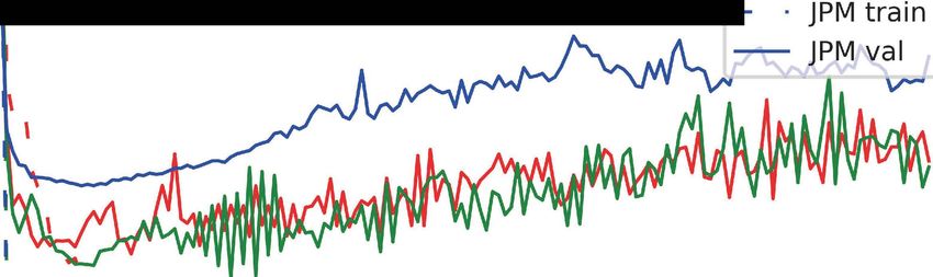
Fig. 2. Training (dash) and validation Fig. 3. Hourly test loss plotted against
(line) loss curves for bid-side models. hourly volume standard deviation.
highest average R-squared, indicating that incorporating temporal information
in both feature vectors and latent state dynamics is the most suitable approach to
capture the model’s dependence on time. Meanwhile we find the model tends to
be overfitting, with validation loss starting to rise before training loss converges.
Fig. 2 shows loss curves for LOBRM (Decay-T) trained with a higher learning
rate of 2e-3. The phenomenon of overfitting also explains why we use a pre-
defined exponential decay kernel instead of a fully flexible ODE kernel involving
a lot more parameters to model temporal dependence. Thus, in the following
experiments, we continue using LOBRM (Decay-T) as the main model.
As shown in Table 2, test losses across 6 sets of experiments fluctuate in
the range [0.332, 0.628] for LOBRM (Decay-T). To test whether this fluctuation
results from order volume volatility, we use the pre-trained model to calculate
the correlation of (hourly) test L1 loss across all experiments against the (hourly)
standard deviation of non-standardized volume resting at deep price levels (see
Fig. 3). We find that the correlation between hourly L1 loss and volume volatility12 Z. Shi and J. Cartlidge
Table 3. Ablation study: test loss.
MSFT INTC JPM Avg.
Bid Ask Bid Ask Bid Ask
HC 6.79 7.42 5.47 6.78 6.22 3.86 6.09
ES 6.31 6.99 5.94 5.70 6.04 3.36 5.72
HC+ES 6.26 6.45 5.40 5.50 6.02 3.32 5.49
HC+ES+WS 6.28 6.15 5.33 5.64 6.18 3.38 5.49
is significant (p-valueExploring the LOB Recreation Model 13
Table 4. LOBRM test loss comparison of explicit and sparse encodings of TAQ data.
MSFT INTC JPM Avg.
Bid Ask Bid Ask Bid Ask
Explicit 6.87 6.43 6.80 9.95 7.60 4.14 6.97
Sparse 6.31 6.99 5.94 5.70 6.04 3.36 5.72
complete TAQ data input and modelling market events as a stochastic process
using a continuous RNN, achieves a lower error than HC module and is the
dominant module that contributes to prediction accuracy. Combining both HC
and ES modules, either using a predefined or adaptive weight, achieves the best
performance, which suggets that the predictions from HC and ES are comple-
mentary and can be effectively combined to gain a higher accuracy prediction.
The purpose of the WS module in the original LOBRM study is to facilitate the
model’s use in transfer learning and it does not contribute to prediction accuracy
when tested on the same stock that it was trained, as is the case here.
4.4 Superiority of Sparse Encoding for TAQ
LOB volume prediction In sparse encoding, only volume information in TAQ
is encoded explicitly and price information are embedded implicitly by positions
of non-zero elements in one-hot vectors. In explicit encoding, information includ-
ing price, volume, and trade direction are encoded directly as non-zero elements
in feature vectors. Here we use the ES module in LOBRM (Decay-T) as the
main model and tested the model prediction accuracy when these two different
encoding methods are used. We don’t choose the full model as explicitly en-
coded input cannot be trimmed so HC module is not used. Results are shown
in Table 4. We see that the model with sparse encoding achieves lower test loss
error in 5 out of 6 experiments. The average test loss for the model with sparse
encoding is 17.9% lower than the model with explicit encoding.
Price trend prediction We compare the sparse encoding method with the
convolution method proposed in [27] for quotes data in the task of stock price
trend prediction. On the basis of explicit encoding, the convolution encoding
method applies two convolution layers with filters of size [1 × 2] and stride [1 × 2]
on quote data. This structure first convolutionalize price and volume information
at ask and bid sides respectively and then convolutionalize two sides’ information
together. We approach a similar task presented in [27] but simplify the model
structure to concentrate on the prediction accuracy variation brought by different
encoding methods. We set length of time series samples as S = 50. For sparse
encoding, we set k = 5. For convolution encoding, we use 16 [1 × 2] kernels with
stride [1 × 2] followed by LeakyReLU activation. We standardize features using
min-max or z-score standardization. Encoded data are passed to an MLP with
ReLU activation. A GRU unit is used to receive iterative inputs and the final
latent state is connected with an MLP with Softmax activation to generate a14 Z. Shi and J. Cartlidge
Table 5. Future price prediction: validation/test accuracy.
Sparse Convolution Convolution
(implicit price) (explicit price) (no price)
Min-max 59.8% / 55.2% 55.9% / 54.4% 57.2% / 53.9%
Z-score 60.2% / 57.4% 57.1% / 54.0% 58.3% / 55.0%
Table 6. LOBRM (Decay-T) test loss against training size.
MSFT INTC JPM Avg.
Bid Ask Bid Ask Bid Ask
Day3 7.15 7.15 6.05 6.18 6.29 3.33 6.03
Day2+3 6.25 6.58 5.86 5.73 6.40 3.32 5.69
Day1+2+3 6.28 6.15 5.33 5.64 6.18 3.32 5.48
possibility distribution over three labels {down, same, up}. We test the model
on MSFT five-day dataset, using first three days for training, the fourth day
for validation, and the fifth day for testing. We run a rolling average of five
timesteps to alleviate label imbalance [19], with 29%, 40%, and 31% for up,
same, and down. We train the model with cross entropy loss for 50 iterations
and choose the model with highest validation accuracy.
Results are shown in Table 5. We can see that the sparse encoding method
with two different standardization methods has superior performance in the task
of price trend prediction, compared with convolution encoding either with or
without price information. Thus, we draw the conclusion that the sparse en-
coding method for TAQ data can not only benefit the task of LOB volume
prediction, but also other tasks including stock price trend prediction.
4.5 Is the Model Well-Trained?
As financial time series suffer from stochastic drift, in the sense that the distri-
bution of data is unstable and tends to vary temporarily, large amounts of data
is needed for model training. For example, the LOB used in [5] and [24] is of
one month’s and seventeen month’s length. Here, for all six sets of experiments
(3 stocks × 2 sides) we use three days’ LOB data for training, one day’s data
for validation, and one day’s data for testing. We would like to test whether this
amount of training data is abundant enough for out-of-sample testing.
As the dataset we possess contains five consecutive trading days’ LOB data,
we leave out the fourth day’s and fifth day’s LOB data for validation and testing.
We first use the third day’s data for training and then iteratively add in the
second and the first day’s historical data to observe how the validation and
testing loss change. Results are shown in Table 6. We can see that there is
a downward tendency in average test loss as more historical data is used for
training. This is especially true for MSFT ask, INTC bid, and INTC ask. This
phenomenon suggests that the influence of stochastic drift may be alleviated byExploring the LOB Recreation Model 15
exposing the model to more historical samples. Therefore, we would expect even
lower out-of-sample errors if more historical data can be used for training.
5 Conclusion
We have extended the research on the LOBRM, the first deep learning model for
generating synthetic LOB data. Two major revisions were proposed: standardiz-
ing LOB data with time-weighted z-score to improve the model’s generalization
ability; and substituting the original ODE kernel with an exponential decay ker-
nel (Decay-T) to improve time efficiency. Experiments were conducted on an
extended LOBSTER dataset, a strict superset of the data used in the original
study, with size approximately ten times larger. Using a fully chronological train-
ing and testing regime, we demonstrated that LOBRM (Decay-T) has superior
performance over traditional models, and showed the efficacy of module ensem-
bling. We further found that: (1) LOB volume prediction accuracy is negatively
related to volume volatility; (2) sparse one-hot positional encoding of TAQ data
can benefit manifold tasks; and (3) there is some evidence that the influence of
stochastic drift can be alleviated by increasing the number of historical samples.
As a whole, this study validates the use of LOBRM in demanding application
scenarios that require efficient inference and involve large amounts of data for
training and predicting.
Acknowledgements Zijian Shi’s PhD is supported by a China Scholarship
Council (CSC)/University of Bristol joint-funded scholarship. John Cartlidge is
sponsored by Refinitiv.
References
1. Abergel, F., Huré, C., Pham, H.: Algorithmic trading in a microstructural limit
order book model. Quantitative Finance 20(8), 1263–1283 (2020)
2. Abergel, F., Jedidi, A.: Long-time behavior of a Hawkes process–based limit order
book. SIAM Journal on Financial Mathematics 6(1), 1026–1043 (2015)
3. Arthur, W.B., Holland, J.H., LeBaron, B., Palmer, R., Tayler, P.: Asset pricing
under endogenous expectations in an artificial stock market. The economy as an
evolving complex system II 27 (1996)
4. Belcak, P., Calliess, J.P., Zohren, S.: Fast agent-based simulation framework of
limit order books with applications to pro-rata markets and the study of latency
effects (2020), arXiv preprint, https://arxiv.org/abs/2008.07871
5. Blanchet, J., Chen, X., Pei, Y.: Unraveling limit order books using just bid/ask
prices (2017), https://web.stanford.edu/~jblanche/papers/LOB_v1.pdf, Un-
published preprint
6. Cartlidge, J., Smart, N.P., Talibi Alaoui, Y.: MPC joins the dark side. In: ACM
Asia Conference on Computer and Communications Security. p. 148–159 (2019)
7. Cartlidge, J., Smart, N.P., Talibi Alaoui, Y.: Multi-party computation mechanism
for anonymous equity block trading: A secure implementation of Turquoise Plato
Uncross (2020), Cryptology ePrint Archive, https://eprint.iacr.org/2020/66216 Z. Shi and J. Cartlidge
8. Che, Z., Purushotham, S., Cho, K., Sontag, D., Liu, Y.: Recurrent neural networks
for multivariate time series with missing values. Scientific reports 8(1), 1–12 (2018)
9. Cho, K., Van Merriënboer, B., Gulcehre, C., Bahdanau, D., Bougares, F., Schwenk,
H., Bengio, Y.: Learning phrase representations using RNN encoder-decoder for
statistical machine translation. In: Conf. on Empirical Methods in Natural Lan-
guage Processing. pp. 1724–1734 (2014)
10. Cont, R., De Larrard, A.: Price dynamics in a Markovian limit order market. SIAM
Journal on Financial Mathematics 4(1), 1–25 (2013)
11. Friedman, D.: The double auction market institution: A survey. The double auction
market: Institutions, theories, and evidence 14, 3–25 (1993)
12. Horst, U., Kreher, D.: A weak law of large numbers for a limit order book model
with fully state dependent order dynamics. SIAM Journal on Financial Mathemat-
ics 8(1), 314–343 (2017)
13. Kumar, P.: Deep reinforcement learning for market making. In: 19th Int. Conf. on
Autonomous Agents and MultiAgent Systems. pp. 1892–1894 (2020)
14. Lechner, M., Hasani, R.: Learning long-term dependencies in irregularly-sampled
time series. In: Ann. Conf. Advances in Neural Information Processing Systems
(2020), preprint available: https://arxiv.org/abs/2006.04418
15. Li, J., Wang, X., Lin, Y., Sinha, A., Wellman, M.: Generating realistic stock market
order streams. In: 34th AAAI Conf. on Artificial Intelligence. pp. 727–734 (2020)
16. Mäkinen, Y., Kanniainen, J., Gabbouj, M., Iosifidis, A.: Forecasting jump arrivals
in stock prices: new attention-based network architecture using limit order book
data. Quantitative Finance 19(12), 2033–2050 (2019)
17. McGroarty, F., Booth, A., Gerding, E., Chinthalapati, V.R.: High frequency trad-
ing strategies, market fragility and price spikes: an agent based model perspective.
Annals of Operations Research 282(1), 217–244 (2019)
18. Nevmyvaka, Y., Feng, Y., Kearns, M.: Reinforcement learning for optimized trade
execution. In: 23rd Int. Conf. on Machine Learning (ICML). pp. 673–680 (2006)
19. Ntakaris, A., Magris, M., Kanniainen, J., Gabbouj, M., Iosifidis, A.: Benchmark
dataset for mid-price forecasting of limit order book data with machine learning
methods. Journal of Forecasting 37(8), 852–866 (2018)
20. Parlour, C.A.: Price dynamics in limit order markets. The Review of Financial
Studies 11(4), 789–816 (1998)
21. Passalis, N., Tefas, A., Kanniainen, J., Gabbouj, M., Iosifidis, A.: Temporal logistic
neural bag-of-features for financial time series forecasting leveraging limit order
book data. Pattern Recognition Letters 136, 183–189 (2020)
22. Rubanova, Y., Chen, T.Q., Duvenaud, D.K.: Latent ordinary differential equations
for irregularly-sampled time series. In: Ann. Conf. Advances in Neural Information
Processing Systems. pp. 5321–5331 (2019)
23. Shi, Z., Chen, Y., Cartlidge, J.: The LOB recreation model: Predicting the limit
order book from TAQ history using an ordinary differential equation recurrent
neural network. In: 35th AAAI Conf. on Artificial Intelligence. pp. 548–556 (2021)
24. Sirignano, J., Cont, R.: Universal features of price formation in financial markets:
perspectives from deep learning. Quantitative Finance 19(9), 1449–1459 (2019)
25. Tsantekidis, A., Passalis, N., Tefas, A., Kanniainen, J., Gabbouj, M., Iosifidis, A.:
Using deep learning for price prediction by exploiting stationary limit order book
features. Applied Soft Computing 93, 106401 (2020)
26. Ye, Z., Florescu, I.: Extracting information from the limit order book: New mea-
sures to evaluate equity data flow. High Frequency 2(1), 37–47 (2019)
27. Zhang, Z., Zohren, S., Roberts, S.: Deeplob: Deep convolutional neural networks
for limit order books. IEEE Trans. on Signal Processing 67(11), 3001–3012 (2019)You can also read