Winter season Southern Ocean distributions of climate-relevant trace gases
←
→
Page content transcription
If your browser does not render page correctly, please read the page content below
Research article
Biogeosciences, 19, 5021–5040, 2022
https://doi.org/10.5194/bg-19-5021-2022
© Author(s) 2022. This work is distributed under
the Creative Commons Attribution 4.0 License.

Winter season Southern Ocean distributions of
climate-relevant trace gases
Li Zhou1 , Dennis Booge1 , Miming Zhang2 , and Christa A. Marandino1
1 Research Division 2: Marine Biogeochemistry, GEOMAR Helmholtz Centre for Ocean Research Kiel, Kiel, Germany
2 KeyLaboratory of Global Change and Marine-Atmospheric Chemistry,
Third Institute of Oceanography, Ministry of Natural Resources (MNR), Xiamen, PR China

Correspondence: Li Zhou (lzhou@geomar.de) and Miming Zhang (zhangmiming@tio.org.cn)

Received: 27 April 2022 – Discussion started: 9 May 2022
Revised: 26 July 2022 – Accepted: 9 August 2022 – Published: 28 October 2022

Abstract. Climate-relevant trace gas air–sea exchange ex-          1   Introduction
erts an important control on air quality and climate, espe-
cially in remote regions of the planet such as the South-
ern Ocean. It is clear that polar regions exhibit seasonal         Despite the low abundance of trace gases in the atmosphere,
trends in productivity and biogeochemical cycling, but al-         their strong chemical reactivity and interactions with radia-
most all of the measurements there are skewed to summer            tion have an important influence on air quality and the cli-
months. If we want to understand how the Southern Ocean            mate system (Monson and Holland, 2001). For example, a
affects the balance of climate through trace gas air–sea ex-       wide variety of trace gases, such as carbon dioxide (CO2 ),
change, it is essential to expand our measurement database         methane, and nitrous oxide, trap heat and contribute to global
over greater temporal and spatial scales, including all sea-       atmospheric warming (Liss, 2007). The ocean plays an im-
sons. Therefore, in this study, we report measured concentra-      portant role in regulating the sources and sinks of trace
tions of dimethylsulfide (DMS, as well as related sulfur com-      gases and, thus, strongly impacts the biogeochemical cy-
pounds) and isoprene in the Atlantic sector of the Southern        cles and budget of reactive trace gases in the global atmo-
Ocean during the winter to understand the spatial and tem-         sphere (Houghton et al., 2001; Liss et al., 2014; Vallina
poral distribution in comparison to current knowledge and          and Simó, 2007). Studying the air–sea exchange of climate-
climatological calculations for the Southern Ocean. The ob-        relevant trace gases can improve the understanding of their
servations of isoprene are the first in the winter season in the   effect on climate (Emerson et al., 1999; Liss et al., 2014).
Southern Ocean. We found that the concentrations of DMS            Here we focus not only on two typical marine biogenic gases,
from the surface seawater and air in the investigated area         i.e., dimethylsulfide (DMS) and isoprene, which have a sig-
were 1.03 ± 0.98 nmol−1 and 28.80 ± 12.49 pptv, respec-            nificant influence on aerosols and climate in remote areas of
tively. The concentrations of isoprene in surface seawater         the world (Carpenter et al., 2012; Lovelock et al., 1972) but
were 14.46 ± 12.23 pmol−1 . DMS and isoprene fluxes were           also on two related sulfur compounds, i.e., dimethylsulfonio-
4.04 ± 4.12 µmol m−2 d−1 and 80.55 ± 78.57 nmol m−2 d−1 ,          propionate (DMSP) and dimethylsulfoxide (DMSO).
respectively. These results are generally lower than the values       DMS was hypothesized to influence climate by regulat-
presented or calculated in currently used climatologies and        ing aerosols and clouds, thus, decreasing the amount of solar
models. More data are urgently needed to better interpolate        radiation reaching Earth’s surface, known as the CLAW hy-
climatological values and validate process-oriented models,        pothesis (Charlson et al., 1987). DMS is produced from the
as well as to explore how finer measurement resolution, both       degradation of DMSP, which is formed in the cells of ma-
spatially and temporally, can influence air–sea flux calcula-      rine organisms (Cantoni and Anderson, 1956; Curson et al.,
tions.                                                             2011). DMSP producers include phytoplankton (e.g., coccol-
                                                                   ithophores, dinoflagellates, diatoms), angiosperms, macroal-
                                                                   gae, and some corals (Broadbent et al., 2002; Keller et al.,

Published by Copernicus Publications on behalf of the European Geosciences Union.
5022                          L. Zhou et al.: Winter season Southern Ocean distributions of climate-relevant trace gases

1989; Otte et al., 2004; Van Alstyne, 2008; Yoch, 2002).         al. (2014) of 0.51–16.53 Tg C yr−1 in June–July 2010 in the
DMSP is cleaved to DMS by bacteria and phytoplankton             Arctic and 9.05–34.96 Tg C yr−1 in the productive Southern
(Curson et al., 2011; Stefels et al., 2007). DMS produced        Ocean during austral summer 2010/11, respectively. Despite
in the surface ocean can be consumed in the ocean, be oxi-       these values being significantly less than the terrestrial flux
dized to form DMSO, or be released to the atmosphere (Vogt       (400–600 Tg C yr−1 ; Arneth et al., 2008; Arnold et al., 2009;
and Liss, 2009). Only about 10 % of the DMS produced in          Baker et al., 2000; Guenther et al., 2006), emitted isoprene in
the surface ocean is released into the atmosphere (Archer et     the marine atmosphere plays an important role in the chem-
al., 2001). DMS in the atmosphere is oxidized to form sul-       istry locally, as it is extremely short-lived (lifetime of ∼ 1 h
furic acid and methanesulfonic acid (McArdle et al., 1998)       due to reaction with OH radicals). Terrestrial isoprene is un-
by hydroxyl radicals (OH; 66 %), nitrate (NO3 ; 16 %), and       likely to reach the marine boundary layer, and all the ma-
bromine monoxide radicals (BrO; 12 %) globally (Chen et          rine isoprene emitted will quickly react (Booge et al., 2018;
al., 2018), with an atmospheric lifetime of approximately        Palmer and Shaw, 2005), influencing local climate and air
1 d (Kloster et al., 2006). These DMS byproducts can form        quality (Claeys et al., 2004).
aerosols (new particles) (Kulmala et al., 2000) or lead to          The fluxes of marine-derived trace gases are an impor-
growth of existing aerosol particles (Andreae and Crutzen,       tant parameter in atmospheric budgets and for the evaluation
1997; von Glasow and Crutzen, 2004), aiding the forma-           of their climate implications. Typically, ocean–atmosphere
tion of cloud condensation nuclei (CCN) (Charlson et al.,        fluxes are calculated by multiplying the wind-speed-based
1987; Sanchez et al., 2018). Especially in the remote marine     gas transfer velocity by the bulk phases of the air–sea con-
boundary layer (MBL) of the North Atlantic and polar oceans      centration difference as follows: F = k1C (Liss and Slater,
(e.g., the Southern Ocean; SO), DMS-derived non-sea salt         1974; see “Methods” section below). Often, only seawater
sulfate particles account for 33 % and 7 %–65 % (7 %–20 %        concentrations are used, and the atmospheric values are set
in winter and 43 %–65 % in summer), respectively (Jackson        either to zero or to a constant level, but this can lead to
et al., 2020; Korhonen et al., 2008; Sanchez et al., 2018).      large uncertainties in calculated fluxes (Lennartz et al., 2017;
Mahmood et al. (2019) show that the mean cloud radia-            Zhang et al., 2020). Thus, having accurate, repeated mea-
tive forcing in the Arctic could increase between 108 % and      surements of trace gases in the surface ocean, as well as in
145 % from 2000 to 2050 because of increasing Arctic DMS         the marine boundary layer, over a range of spatial and tem-
emissions. The global radiative effect of DMS is calculated      poral scales is necessary for high-quality flux computations.
to be −1.69 to −2.03 W m−2 at the top of the atmosphere             The Global Surface Seawater DMS Database contains
(Fiddes et al., 2018; Mahajan et al., 2015; Thomas et al.,       89 324 measurements of surface ocean DMS concentration
2010). These previous studies clearly show the importance        from 1972 to 2019 (https://saga.pmel.noaa.gov/dms/, last ac-
of DMS emissions and related atmospheric oxidation prod-         cess: 23 January 2022). Concentrations of oceanic DMS
ucts and point to the importance of understanding how global     within the database range between 0 and 295 nmol L−1 . The
DMS concentrations and subsequent emissions vary over the        broader Southern Ocean (latitude range: 35 to 75◦ S) is rep-
course of the year and over longer time periods.                 resented by 21 580 points for all seasons, but only 158 points
   Isoprene is the most important biogenic volatile organic      (0.7 %) are from the austral winter. All three DMS clima-
compound (BVOC) in the atmosphere, accounting for 50 %           tologies draw heavily on this database (Hulswar et al., 2022;
of all BVOC emissions coming from terrestrial ecosys-            Kettle et al., 1999; Lana et al., 2011). This DMS data product
tems (Guenther et al., 2012; Laothawornkitkul et al., 2009;      and resulting climatologies, along with those for other trace
Sharkey et al., 2008). It impacts the climate system and         gases (MEMENTO, MarinE MethanE and NiTrous Oxide;
oxidant chemistry in the atmosphere via secondary organic        SOCAT, Surface Ocean CO2 Atlas; HalOcAt, Halocarbons
aerosol (SOA) formation and interaction with OH and the          in the Ocean and Atmosphere; among others), are extremely
ozone cycle (Claeys et al., 2004; Guenther et al., 1995; Went,   important for model input and validation. If the data prod-
1960). Most isoprene in the atmosphere is produced by ter-       ucts contain the appropriate data, they can resolve seawater
restrial ecosystems (> 99 %, Guenther et al., 2006), but iso-    concentrations spatially and temporally (e.g., seasonally), as
prene is also known to be produced in the ocean as well          well as begin to point to interannual variability and trends.
by different species of phytoplankton, seaweed (Shaw et          Therefore, these valuable assets must be equipped with as
al., 2003; Bonsang et al., 1992), and some species of ma-        much data from all regions and seasons as possible. Lana et
rine bacteria (Exton et al., 2013). Since atmospheric iso-       al. (2011), the most currently used DMS climatology, show
prene in remote regions of the open ocean are directly re-       that DMS concentrations typically range from 1–7 nmol L−1 ,
lated to surface seawater isoprene concentrations (Bonsang et    with higher concentrations occurring in the high-latitude re-
al., 1992), biological marine isoprene production directly in-   gions with strong seasonality. The highest DMS concentra-
fluences the magnitude of emissions to the atmosphere. The       tions appear in the high-latitude provinces of the North At-
global marine flux of isoprene is reported to range from 0       lantic and North Pacific in summer, with DMS concentra-
to 11 Tg C yr−1 (Booge et al., 2016), with more extreme          tions generally increasing with temperature and light and
values reported by Tran et al. (2013) and Kameyama et            sometimes exceeding 20 nmol L−1 (Lana et al., 2011). In

Biogeosciences, 19, 5021–5040, 2022                                                 https://doi.org/10.5194/bg-19-5021-2022
L. Zhou et al.: Winter season Southern Ocean distributions of climate-relevant trace gases                                    5023

the temperate and subtropical provinces, the seasonality be-           The Southern Ocean is a typical high-nutrient and low-
comes weaker, until around the Equator, where there is no           chlorophyll area due to iron limitation, which exerts a strong
obvious seasonal change. The transition to the southern sub-        influence on global biogeochemical cycles and air–sea gas
tropical zone shows weaker seasonal changes, but in aus-            fluxes (Hauck et al., 2013; Zhang et al., 2017). Knowledge of
tral summer, the Southern Ocean circumpolar regions dis-            the general biological productivity and circulation patterns of
play a hotspot of DMS concentrations (> 10 nmol L−1 ) (Mc-          the area has made great advances; however, it is still difficult
Taggart and Burton, 1992). Lana et al. (2011; abbreviated           to resolve the small-scale dynamics of gases in the surface
as Lana below) estimated that approximately 28.1 Tg S are           (Tortell and Long, 2009), especially during the wintertime.
transferred from the oceans into the atmosphere annually in         If we want to understand how the Southern Ocean effects on
the form of DMS. The natural sulfur emission has been esti-         the balance of climate through trace gas air–sea exchange, it
mated as 38–89 Tg S yr−1 (Andreae, 1990), of which marine           is essential to expand our measurement database over greater
DMS emission contributes 30 %–70 %. Although there were             temporal and spatial scales, including all seasons. Therefore,
many field campaigns performed, the obtained oceanic DMS            in this study we measured the concentrations of DMS; its
data are still insufficient, leaving uncertainties about sea-to-    precursor, DMSP, and oxidation product, DMSO; and iso-
air DMS fluxes, especially during the winter season. In the         prene in the Southern Ocean during the austral winter season
Lana climatology, Southern Ocean data are skewed to spring          to gain information on the spatial and temporal distribution
and summer and are spatially non-uniform, requiring the use         in comparison to current knowledge and climatological cal-
of interpolation/extrapolation techniques. Thus, it is unavoid-     culations for the Southern Ocean.
able that large discrepancies between fluxes calculated in situ
vs. those in the climatology are found (even at levels as high
as 47 %–76 %, Zhang et al., 2020). Better spatial and tempo-        2     Methods
ral coverage of in situ measurements are needed for adequate
                                                                    2.1    Cruise description
computations of the influence of DMS on global climate.
   Marine production and emission of isoprene were first de-        The measurements were performed on the Southern oCean
scribed by Bonsang et al. (1992). Currently published iso-          seAsonaL Experiment (SCALE) cruise aboard the S. A. Ag-
prene seawater values from the world oceans generally range         ulhas II. The cruise started from Cape Town, Republic of
from below 1 to 200 pmol L−1 (Baker et al., 2000; Bon-              South Africa (RSA), on 18 July 2019 (199th day of year,
sang et al., 1992; Booge et al., 2016; Broadgate et al., 1997,      DOY 199), crossed the Southern Ocean to the ice edge, and
2004; Hackenberg et al., 2017; Li et al., 2019; Matsunaga           returned from the ice area on 28 July 2019 (DOY 209) to
et al., 2002; Milne et al., 1995; Ooki et al., 2015; Zindler        dock in Cape Town on 11 August 2019 (DOY 223) via the
et al., 2014). The highest reported concentration of isoprene,      East London port from 7–10 August 2019 (DOYs 219–222)
541 pmol L−1 , in the surface ocean was found in the Arctic         (33–58◦ S, 2◦ W–26◦ E, Fig. 1). Wind speeds ranged between
Ocean in June–July 2010 (Tran et al., 2013). Marine isoprene        1.2 and 29.4 m s−1 over the cruise. Air mass back trajectories
concentrations in the eastern North Pacific range from 2            show that the air was of oceanic origin for most of the cruise.
to 6.5 pmol L−1 , which is at the lower end compared to the         Air temperatures ranged from −19.5 to +18 ◦ C; sea surface
world oceans (Moore and Wang, 2006). Additionally, con-             temperatures (SSTs) were from −1.8 to +20.4 ◦ C; and salin-
centrations of marine isoprene show strong seasonal changes         ity was 19.4–35.3 over the cruise track.
in regions with strong seasonal variations in phytoplankton
abundances, e.g., in the East China Sea (Li et al., 2018).          2.2    Sampling
Booge et al. (2016) improved the predictive capability of the
earlier model from Palmer and Shaw (2005) by using iso-             Discrete surface seawater samples for DMS and isoprene
prene production rates that depend on phytoplankton func-           were taken bubble-free using transparent 60 mL glass vials
tional type, but the model is still limited, as it cannot resolve   (Chromatographie Handel Müller, Fridolfing, Germany)
changes in isoprene emissions on short timescales of hours or       from the underway pump supply. The water samples were
days. Additionally, the model is validated with a very sparse       kept in a dark, insulated box and analyzed within 2 h. After
dataset presently, which cannot resolve seasonal changes in         analysis, DMSP was converted into DMS using sodium hy-
isoprene concentrations for the world oceans. Especially in         droxide (NaOH) pellets (≥ 99 %, Carl Roth™ GmbH, Karl-
the Southern Ocean, which is thought to be a hotspot of trace       sruhe, Germany) and stored for DMSP and DMSO measure-
gas emissions during austral summer, data are limited. There        ments back in the onshore lab.
are no observations during winter published for this area.             Our sampling frequency for DMS and isoprene was one
Therefore, it is of fundamental importance to increase the          sample per hour at the beginning of the cruise. We changed
dataset of marine isoprene concentrations to understand the         to one sample per 30 min during the last 2 d of the cruise be-
magnitude of the influence of marine isoprene emissions on          cause the concentrations of DMS and isoprene were more
atmospheric processes over the Southern Ocean.                      variable in the coastal area. DMSP–DMSO samples were
                                                                    taken every 2 h. We obtained 384 discrete samples of DMS

https://doi.org/10.5194/bg-19-5021-2022                                                    Biogeosciences, 19, 5021–5040, 2022
5024                            L. Zhou et al.: Winter season Southern Ocean distributions of climate-relevant trace gases

Figure 1. The cruise track (black) superimposed on satellite data. (a) Sea surface temperature (SST) and ice coverage (%). SST and sea ice
data are derived from satellite (12 July to 12 August 2019; SST – Naval Oceanographic Office, 2008; sea ice data – UK Met Office, 2012.);
(b) 24 h air mass back trajectories starting at 50 m height from HYbrid Single-Particle Lagrangian Integrated Trajectory (HYSPLIT) using
the meteorological fields from the National Centers for Environmental Prediction Global Data Assimilation System (NCEP GDAS). The
color shows the average height of the trajectory.

and isoprene and 204 samples of DMSP–DMSO during the                   2.3   Analysis
cruise. During the cruise, the seawater pumping system was
stopped due to the presence of sea ice on 27–28 July 2019
(DOYs 208–209) and while in port of East London (7–10 Au-              DMS, DMSP, DMSO, and isoprene were analyzed by gas
gust 2019, DOYs 219–222), resulting in periods with missing            chromatography–mass spectrometry (GC–MS) coupled to
data.                                                                  a purge-and-trap system. Headspace within each sample
   We also performed continuous shipboard underway mea-                was made by injecting 10 mL of helium into the vial. Iso-
surements of surface water and lower-atmospheric DMS us-               prene was fully removed from the remaining 50 mL sam-
ing a homemade purge-and-trap sampler coupled with a                   ple (> 99 %) with helium at a flow rate of 70 mL min−1 for
time-of-flight mass spectrometer system (TOF-MS 3000,                  15 min at room temperature (RT). Purge efficiency for DMS
Guangzhou Hexin Instrument Co., Ltd., China) (Zhang et                 was less than 100 % and dependent on the seawater temper-
al., 2019). Seawater and air samples were introduced con-              ature, but the data were corrected for this effect (Fig. S1).
tinuously to the system through the ship’s seawater pump               Gaseous deuterated isoprene (isoprene-d5; 98 %) was used
system and air sampler inlet located at the bow at approx-             as internal standard and injected through a 500 µL Sulfinert®
imately 18 m above the sea surface. A black antistatic tube            stainless-steel sample loop (1/16 in. o.d., Restek, Bad Hom-
(1/4 in. o.d., 95 m) was used to transport the air sample to           burg, Germany). The sample flow was dried using a Nafion®
the laboratory. Every 10 min, we obtained a pair of DMS data           membrane dryer (counter flow: N2 , 180 mL min−1 , Perma
points (one in seawater and one in the atmosphere). For sea-           Pure, Ansyco GmbH, Karlsruhe, Germany). After purging,
water sample measurements, we purged a 5 mL aliquot with               DMS and isoprene were trapped in a Sulfinert® stainless-
65 mL min−1 of high-purity nitrogen (N2 ) for 5.5 min. For at-         steel trap cooled with liquid N2 . The sample was injected
mospheric DMS measurements, the air sample was trapped                 into the GC by immersion in hot water. Retention times
under the mean flow at 65 mL min−1 for 3.5 min. The con-               for DMS and isoprene (m/z: 61, 62; 67, 68) were 5.0 and
centrated air sample was injected to the TOF-MS system;                5.3 min. For analysis of DMSP, 10 mL of the DMS sample
then 2 min later the concentrated water sample was injected            was transferred to brown glass vials (Chromatographie Han-
to the TOF-MS system. The atmospheric and seawater DMS                 del Müller, Fridolfing, Germany). After the DMSP analy-
limits of detection (LODs) were 32 pptv and 0.07 nmol L−1 ,            sis, DMSO was converted into DMS by adding cobalt-dosed
respectively.                                                          sodium borohydride (NaBH4 ) (90 %, Sigma-Aldrich Chemie
                                                                       GmbH, Taufkirchen, Germany) and analyzed immediately
                                                                       with the same technique as mentioned above. Liquid stan-
                                                                       dards and an internal standard were used to calibrate the
                                                                       system for DMS and isoprene every day during the analysis

Biogeosciences, 19, 5021–5040, 2022                                                        https://doi.org/10.5194/bg-19-5021-2022
L. Zhou et al.: Winter season Southern Ocean distributions of climate-relevant trace gases                                       5025

on board. Liquid calibrations were performed every measur-       and is set to 0.11 (Hsu et al., 1994). Sc is defined as the ratio
ing day for the DMSP–DMSO analysis in the lab. The given         of the kinematic viscosity of water to the diffusion coeffi-
LODs of this system are 10 times the standard deviation of       cient of gas in water, and 660 represents CO2 in seawater at
the baseline noise, which are 1.8×10⁻¹³ and 5.5×10⁻¹³ mol        20 ◦ C. We estimate Sc of DMS and isoprene following Wan-
for DMS and isoprene, respectively.                              ninkhof (2014) and Palmer and Shaw (2005), respectively:
   Continuous underway measurements of SST and salinity,
as well as wind speed and direction, air temperature, pres-      ScDMS = 2855.7 − 177.63 Tc + 6.0438 Tc 2
sure, and global radiation, were recorded from the ship’s                   − 0.11645 Tc 3 + 0.00094743 Tc 4 ,                     (7)
pumped seawater supply and the meteorological tower, re-
                                                                                                                     2
spectively.                                                      Scisoprene = 3913.15 − 162.13 Tc + 2.67 Tc
                                                                               − 0.012 Tc 3 ,                                      (8)
2.4   Calculation of air–sea flux
                                                                 where Tc is SST (◦ C).
The air–sea fluxes of all gases were calculated with Eq. (1):
                                                                   In addition, for DMS, the partitioning of the gas transfer
                                                                 coefficient between air-side and water-side control (γa ) can

                                          Ca
F = (1 − A)k · 1C = (1 − A)k · Cw −            ,           (1)   change due to low SSTs and from moderate wind speeds
                                          H
                                                                 (McGillis et al., 2000). Thus, we consider both water-side
where F is the flux (per mass area per time), A is fraction of   and air-side control when calculating DMS fluxes:
sea surface covered by ice, 1C is the concentration differ-
ence between air (Ca ) and water (Cw), k is the gas exchange     F = (1 − A) kw (1 − γa ) · 1C,                                    (9)
coefficient (m s−1 ) in water (Liss and Slater, 1974), and H
is the Henry’s law coefficient used to calculate gas solubil-    where A is the fraction of sea ice cover and γa is calculated
ity. The gas exchange coefficient for the gases of interest is   as
usually approximated as the water–air side transfer velocity,                 1
kw . We use the following parametrizations derived from dual     γa =                ,                                            (10)
                                                                        1 + αkkaw
tracer (Nightingale et al., 2000; N00) and eddy covariance
direct measurement of air–sea DMS transfer (Zavarsky et al.,     where ka is air-water side transfer coefficient and α is the
2018; Z18) to calculate the DMS gas transfer velocity fol-       Ostwald solubility coefficient. These parameters were calcu-
lowing Eqs. (2) and (3):                                         lated as described in McGillis et al. (2000) and the references
                                    Sc −0.5                  therein as
                      2
kDMS,N00 = 0.222 · U + 0.333 · U                ,          (2)                         −0.5
                                      660

                                                                                  M
                                                                 ka ≈ 659U10                 ,                              (11)
                               Sc −0.5

                                                                                 MH2 O
kDMS,Z18 = (2.00 · U + 0.94)            .                  (3)          h                  i
                               660                                          3525
                                                                            T (K) −9.464
                                                                 α=e                           ,                                  (12)
   We use the Wanninkhof (1992; W92) and Wan-
ninkhof (2014; W14) formulations, based on a synthesis of        where M is the molecular weight of DMS or H2 O and T
tracer, wind–wave tank, radon, and radiocarbon studies to de-    is the seawater temperature (K). Finally, as no atmospheric
termine kisoprene (Eqs. 4 and 5):                                measurements of isoprene were obtained, we assume Ca of
                                                                 isoprene is zero in the remote MBL due to its very short life-
                             Sc −0.5                             time. Two wind-speed-based gas transfer parameterizations

kisoprene,W92 = 0.31 · U 2           ,                     (4)   for each gas were used, and the respective fluxes were com-
                            660
                                                                 pared to each other and to existing climatologies or model
                               Sc −0.5

kisoprene,W14 = 0.251 · U 2            ,                   (5)   calculations. For DMS, N00 was used for direct comparison
                              660                                to the Lana climatology and Z18 because it is known that
where U is the wind speed at 10 m height and Sc is the           DMS exhibits mostly interfacial gas transfer, which is more
Schmidt number. The wind was measured at 18 m height and         accurately described with a linear wind speed dependence.
converted to 10 m using                                          For isoprene, we used parameterizations with a quadratic de-
                                                                 pendence on wind speed, since it is less soluble than DMS
         Zx P                                                    and likely to have more influence from bubble-mediated gas

 Ux
    =            ,                                    (6)        transfer. W92 was chosen for direct comparison with Palmer
U10      Z10
                                                                 and Shaw (2005) and Booge et al. (2016), but the more ac-
where Ux is the observed wind speed at 18 m; Zx and Z10          curate version of this parameterization is W14, and, thus, it
are heights of 18 and 10 m, respectively; and P depends on       was also used for comparison.
atmospheric stability and underlying surface characteristics

https://doi.org/10.5194/bg-19-5021-2022                                                            Biogeosciences, 19, 5021–5040, 2022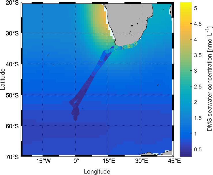
5026                            L. Zhou et al.: Winter season Southern Ocean distributions of climate-relevant trace gases

2.5    Data analysis

The data were tested for normal distribution using the
Kolmogorov–Smirnov test and was determined to be non-
normally distributed. Outliers were identified as deviating
more than 3 times from the standard deviation of the mean.
We used Spearman correlation analysis to identify corre-
lation coefficients between DMS, DMSP, and DMSO. The
F statistic, p value (significance), R (correlation coefficient),
and R 2 (variance proportionality) were calculated to test for a
linear correlation between two variables. All statistical anal-
yses were performed using MATLAB (The MathWorks, Inc.,
Natick, Massachusetts, United States).

3     Results and discussion

3.1    Comparison of DMS measurements by GC–MS
       and TOF-MS

Simultaneous measurements of surface seawater DMS con-
centrations during SCALE were performed using both the
GC–MS and TOF-MS systems. We ensured method com-
parability by using the same DMS standards (both gas and
liquid) on board. We collected 361 GC–MS samples and
2245 TOF-MS samples during the in situ observations. Al-            Figure 2. The (a) correlation and (b, c) Gaussian distribution anal-
though the detection limit of the GC–MS system is lower             ysis of DMS concentrations measured by TOF-MS (b) and GC–MS
than that of the TOF-MS system, the time resolution of the          (c). TOF-MS data were matched to GC–MS data within a ±5 min
TOF-MS system is higher. Considering the different time res-        timing interval. The black line and red line in (a) denote the regres-
                                                                    sion line and the 1 : 1 line, respectively. The red lines in (b) and (c)
olution of the two instruments, we only compare the data
                                                                    denote the density curve.
of samples taken at the same time (258 data points). The
datasets were found to be correlated and agreed well with
each other (Fig. 2a, p < 0.01, slope = 0.91, R = 0.67). The
median and mean values of TOF-MS observations are higher,           3.2   Environmental characterization during SCALE
42.5 % and 12.9 %, respectively, than those by GC–MS
(Fig. 2b). This may be due to the fact that the TOF-MS sys-         The cruise started in the Atlantic Ocean, at Cape Town, and
tem does not have a column that separates isomers and can-          sailed, crossing different fronts, to the Southern Ocean ice
not distinguish between compounds of the same mass num-             zone before returning along almost the same track, via East
ber, making the mean and median values higher than GC–              London, back to Cape Town (Fig. 1). According to the ratio
MS. Alternatively, we observed that 95 % of the DMS con-            of SST and salinity along the track, three different regions
centrations in both instruments were less than 1.7 nmol L−1         were identified, namely the subtropical, Antarctic Circum-
and that in this concentration range, the slope of the fit is       polar Current (ACC), and Antarctic regions (Fig. 3; see the
slightly lower than the 1 : 1 line. This may reflect added          Supplement for more details on the defining characteristics;
uncertainty from the GC–MS purge efficiency correction.             Fig. S2). At DOYs 201.91 and 216.01, we observed a change
The regions of the cruise track corresponding to these lower        between the ratios greater than 0.05 but did not find such a
concentrations were the coldest regions encountered, corre-         strong change at other observation points, thus distinguishing
sponding to the highest solubilities. Thus, the GC–MS val-          the subtropical and ACC regions. For the Antarctic region,
ues may be too low in this concentration range. As it is not        we found that the ratio of change intensity was not as strong
clear which set of measurements were incorrect and given the        as between subtropical and ACC but did occur (a change
very good agreement, we decided to use the data in following        of 0.04). From this ratio, we distinguish the two regions of
way: fluxes were computed over the entire cruise track, using       ACC and Antarctic. Luis and Lotlikar (2021) report that the
GC–MS measurements for seawater DMS concentrations, as              range of SST in the ACC region is from 1.8 to 9 ◦ C, and that
the same instrument was used to perform DMSP and DMSP               of salinity is from 33.85 to 34.8; the SST of the Antarctic
measurements. TOF-MS measurements were used for atmo-               area is less than 1.5 ◦ C, and the salinity is less than 34. These
spheric mixing ratios.                                              ranges are consistent with our SST–salinity-ratio-defined re-

Biogeosciences, 19, 5021–5040, 2022                                                      https://doi.org/10.5194/bg-19-5021-2022
L. Zhou et al.: Winter season Southern Ocean distributions of climate-relevant trace gases 5027
gions. Unfortunately, in the ice area (DOYs 208.4–209.8), The average sea surface concentration of DMSP during
surface seawater was not collected, because the inlet of the the observation period was 11.26 ± 6.98 nmol L−1 , and the
underway pump was blocked by the sea ice. The underway distribution range was 3.73–40.27 nmol L−1 (Fig. 4b). By
pump was shut down also when the ship docked at the port of comparing to previous research, it can be seen that the con-
East London (DOYs 219.4–222.4). The lowest air tempera- centration during the entire observation period is lower than
ture occurred at DOY 208, which was approximately −20 ◦ C most of the existing literature values, likely because biolog-
(Fig. 3c). During the cruise, wind speed (Fig. 3b) was on av- ical activity in winter is low, resulting in the lowest concen-
erage 15.0 ± 2.5 m s−1 . We experienced higher wind speeds tration of DMSP (Curran et al., 1998; Jones et al., 1998;
between DOYs 210 and 214 and DOYs 216–217, averag- Kiene et al., 2007). The only values that are similarly low
ing over 20 m s−1 . As the ship approached the coast, winds are also from the winter season (Cerqueira and Pio, 1999).
slowed down, and air temperatures rose. The highest concentrations were found in the subtropical re-
gion (average: 16.48 ± 7.08 nmol L−1 ). Average concentra-
3.3 Distribution of dissolved DMS and related tions in the ACC and Antarctic regions were 9.00 ± 3.44 and
compounds 5.19 ± 0.94 nmol L−1 , respectively.
The average sea surface concentration of DMSO dur-
During the campaign, the mean sea surface concentration ing the observation period was 5.41 ± 5.31 nmol L−1 , and
of DMS was 1.03 ± 0.98 nmol L−1 using the GC–MS sys- the distribution range was 1.18–33.56 nmol L−1 (Fig. 4b).
tem (0.75 ± 0.52 nmol L−1 , TOF), ranging from 0.26 to The subtropical region had the highest average concentration
5.18 nmol L−1 (0.21–3.96 nmol L−1 , TOF, Fig. 4a). The con- of 9.28 ± 6.15 nmol L−1 , and the average concentrations of
centrations measured during SCALE are comparable to those the ACC and Antarctic regions were similar, 2.74 ± 1.17 and
from previous winter measurements (Table 1). Measure- 1.90 ± 0.52 nmol L−1 , respectively. Kiene et al. (2007) mea-
ments made at lower latitudes appear to be consistently sured the concentration of dissolved DMSO in the Southern
higher than those made at higher latitudes. Surface seawa- Ocean in the summer of 2009, and the concentration range
ter DMS levels in the Southern Ocean during winter were (1–55 nmol L−1 ) was higher than the concentration of total
much lower than those measured in spring (e.g., 0.4–7.9 DMSO in this study. Our study area was not subject to human
and 3–40 nmol L−1 , Curran and Jones, 2000; Kiene et al., interference, and the biological activity, as well as light lev-
2007), summer (e.g., 0.6–30 nmol L−1 , Tortell and Long, els, in winter is low; therefore our wintertime measured con-
2009), and autumn (e.g., 0.7–3.3 nmol L−1 and not detected centrations can be regarded as the lowest background value
(nd) to 27.9 nmol L−1 , Wohl et al., 2020; Yang et al., 2011; of the area.
Zhang et al., 2020). The average concentration in the sub-
tropical region was the highest during the entire cruise, 3.4 Relationships between sulfur compounds
which was 1.86 ± 1.05 nmol L−1 , while the average concen-
trations in the ACC and Antarctic regions were significantly Correlation analysis of DMS and DMSP–DMSO in differ-
lower, 0.48 ± 0.15 and 0.36 ± 0.04 nmol L−1 , respectively. ent circulation regions (Fig. 6) shows that the regional re-
The southern and northern ACC transects and the Antarc- lationships are different. In the subtropical area, the slopes
tic regions presented a similar concentration range between of DMS against DMSP–DMSO are similar, with p values
0.26 and 1.00 nmol L−1 ; however, over the two observation less than 0.01 and R 2 values higher than 0.5. Studies have
periods of the subtropical region, the concentration ranges of shown that DMSO can be a source of DMS in areas with
DMS were not similar. The subtropical region along the first strong sunlight (Zindler et al., 2015). Therefore, in the sub-
transect (southwards) exhibited lower concentrations than tropical area, the source of DMS relates to both DMSP and
the same area of the second transect (northwards). This dif- DMSO. The slope of DMSP against DMSO is 0.64, with a
ference could be due to the duration of time spent sampling p value less than 0.01 and R 2 = 0.6 (Fig. 6c). This infor-
at the coast: at the beginning of the cruise, the coastal zone mation, along with the similar concentration range for both
was left behind relatively quickly, while on the return trip, a DMSO and DMSP (ca. 40 nmol L−1 ), indicates a tight cou-
greater period of time was spent sampling the near-shore wa- pling between DMSP and DMSO. Overall, the positive corre-
ters. Fluctuations in DMS concentrations were visible where lation between DMS, DMSP, and DMSO indicates that there
the subtropical region and the ACC circulation met, along is strong cycling between the three in this region.
with SST and salinity changes. Finally, in order to understand We further split the subtropical data into coastal (blue dots,
uncertainties induced by sparse sampling in winter, we com- Fig. 6a–c) and open ocean (red dots, Fig. 6a–c), as we see
pare our data to the Lana climatology (Lana et al., 2011). We that there is a distinct concentration difference in these sub-
have calculated that our values are 2.2±0.4 times lower than regions. We again analyzed the relationship between DMS,
the values of Lana et al. (2011) in the open-ocean regions of DMSP, and DMSO in these two areas, and we find that
our cruise track. However, in the coastal area the described the concentration of DMS, DMSP, and DMSO is higher at
values in Lana et al. (2011) is 1.6 ± 1.0 times lower than our the coasts than in the open ocean. The R 2 values between
measured values in the same area (Fig. 5). DMS and DMSP are 0.81 and 0.38 in open seas and near-
https://doi.org/10.5194/bg-19-5021-2022 Biogeosciences, 19, 5021–5040, 20225028 L. Zhou et al.: Winter season Southern Ocean distributions of climate-relevant trace gases
Figure 3. Auxiliary parameters. In situ measurements of (a) salinity, (b) wind speed at 18 m (black) and light levels (red), (c) air temperature
(black) and SST (red), and (d) cruise track latitude (black) and cruise track longitude (red) averaged over 10 min. The bars across the top of
the figure denote the different hydrographic regions discussed throughout the text.
Table 1. Literature review of published field studies of DMS concentrations and mixing ratios (seawater, air) during wintertime (SO: Southern
Ocean; O: open ocean; I: island; C: coastal).
Reference Area Water type DMSwater (nmol L−1 ) DMSair (pptv)
Mean Range Mean Range
Lee and De Mora (1996) New Zealand O, C 1.82 1.51–2.82
Nguyen et al. (1992) Amsterdam Island (Indian Ocean) C, I 0.20 13.20
Gibson et al. (1988) Antarctic O, C 1.38 1.11–1.64
Nguyen et al. (1990) Southern Indian Ocean O, C 2.51 0.30–2.01 58 34–274
Akademik Korolev (1987), unpublished Indian and Pacific oceans O 0.75 0.31–1.25 1.25
Marion Dufresne (1998), unpublished Indian Ocean O 0.96 0.37–2.01 2.01
This study SO: whole cruise O 1.03 ± 0.98 0.26–5.18 28.80 ± 12.49 0.06–88.68
SO: subtropical region 1.86 ± 1.05 0.45–5.18 23.25 ± 7.16 7.49–35.71
SO: ACC region 0.48 ± 0.15 0.30–1.00 29.16 ± 9.41 0.06–58.34
SO: Antarctic region 0.36 ± 0.04 0.26–0.47 31.40 ± 16.77 0.06–88.68
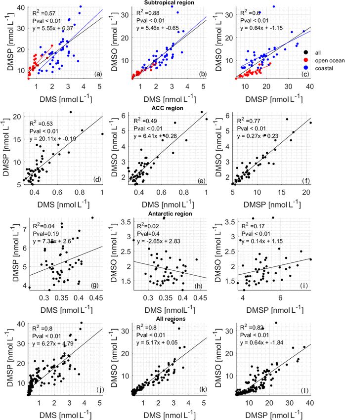
coast areas, and the slopes are 8.14 and 7.13, respectively. al., 2002), the relationship between the two compounds may
The p values are less than 0.01 for both subregions. This be confounded by DMS interconversion with DMSO (as dis-
result shows that closer to the subtropical coastal area, the cussed below). The R 2 values between DMS and DMSO in
DMSP has a positive effect on DMS, with a lesser impact the open-ocean and the coastal regions are 0.77 and 0.61;
in the open sea. While it has been shown that more micro- the p values are less than 0.01; and the slopes are 3.61 and
bial DMSP cleavage to DMS occurs at the coast (Zubkov et 6.02, respectively. The obvious difference in correlation and
Biogeosciences, 19, 5021–5040, 2022 https://doi.org/10.5194/bg-19-5021-2022L. Zhou et al.: Winter season Southern Ocean distributions of climate-relevant trace gases 5029
Figure 4. (a) Measured DMS concentrations in seawater using both instruments; (b) measured DMSP and DMSO concentrations in the sea
surface using the GC–MS system. The bars across the top of the figure denote the different hydrographic regions discussed throughout the
text.
DMSO is higher at the coast, not because of direct algal pro-
duction of DMSO along with DMSP but because there is
more DMSP to DMS microbial cleavage (Fig. 6a) and strong
cycling between DMS and DMSO due to enhanced photo-
chemistry (Fig. 6b) – where DMSP is high because of greater
biological productivity (Hatton et al., 2004, 2012; Stefels et
al., 2007).
The concentration range of DMS, DMSP, and DMSO in
the ACC region is reduced by half or even more than that of
the subtropical area. In addition, it can be seen that the slope
(20.1) between DMS and DMSP is significantly higher than
that between DMS and DMSO or DMSP and DMSO. The
p value is less than 0.01, and the R 2 value is greater than 0.5,
indicating that DMSP has a leading role in the generation of
DMS. The higher slope means that more DMSP is required in
the ACC region to produce DMS compared to the subtropical
region. This again may indicate different microbial pathways
Figure 5. Comparison between measured DMS concentrations leading to higher DMS production in the subtropical area.
(cruise track trace) and those in the Lana et al. (2011) climatology In the Antarctic circulation area, the p values between
(background) for August. DMS and DMSP, DMS, and DMSO are all greater than 0.01,
indicating that the sources of DMSP and DMSO are not con-
nected. Although the p value between DMSP and DMSO
is less than 0.01, the R 2 value is only 0.17, supporting the
slope indicates that the relationship is different, possibly be- idea that the cycling of the compounds is relatively decou-
cause the coastal region may contain more photosensitizers pled (Fig. 6, Antarctic region). There appears to be little to no
(CDOM, chromophoric dissolved organic matter; FDOM, biological activity there. Additionally, due to the low dose of
fluorescent dissolved organic matter) promoting increased solar radiation during winter in the Southern Ocean (Fig. 3g),
photochemical cycling between the two compounds (Mop- little DMSO production via photoreaction from DMS is ex-
per and Kieber, 2002). Comparing the relationship between pected (Vallina and Simó, 2007).
DMSP and DMSO, we find that in the near-coast area, the Simó et al. (2000) found that the relationship between
R 2 value between DMSP and DMSO is 0.50, while in the DMSPp : DMSOp and SST points to the presence of coc-
open sea it is 0.76; the p values are less than 0.01, and the colith blooms that lead to high levels of DMSP. Simó and
slopes are 0.49 and 0.37, respectively. This may indicate that
https://doi.org/10.5194/bg-19-5021-2022 Biogeosciences, 19, 5021–5040, 20225030 L. Zhou et al.: Winter season Southern Ocean distributions of climate-relevant trace gases Figure 6. Correlations between measured DMSP and DMS (the left column of the figure), DMSO and DMS (the middle column of the figure), and DMSO and DMSP (the right column of the figure): (a–c) subtropical region (black points), (d–f) ACC region, (g–i) Antarctic region, and (j–l) entire cruise. The red points in (a)–(c) are data from the open ocean in the subtropical area, and the blue points are data from the subtropical area near the coast. The results of the correlation analysis between DMS and DMSP are R 2 = 0.81, p < 0.01, y = 8.14x+5.01 for open-ocean waters and R 2 = 0.38, p < 0.01, y = 7.13x + 1.9 for coastal waters. The results of the correlation analysis between DMS and DMSO are R 2 = 0.77, p < 0.01, y = 3.61x + 1.12 for open-ocean waters and R 2 = 0.61, p < 0.01, y = 6.02x − 2.04 for coastal waters. The results of the correlation analysis between DMSP and DMSO are R 2 = 0.76, p < 0.01, y = 0.37x − 0.11 for open-ocean waters and R 2 = 0.5, p < 0.01, y = 0.49x + 3.26 for coastal waters. Vila-Costa (2006) found that the particulate DMSP (DMSPp) atures until about 5 ◦ C and then a decreasing relationship in and DMSO (DMSOp) ratio has a negative correlation with warmer waters. The relationship between total DMSP (DM- SST and latitude. Zindler et al. (2013) found that the trend SPt) and DMS to SST over the entire cruise was also inves- changes sign at temperatures below 5 ◦ C. The temperature in tigated (Fig. S3). The pattern observed in DMSPt : DMSOt our observation area varies widely, so it is a good dataset for associated with SST above 5–10 ◦ C is likely due to the varia- determining if this change in relationship with SST is robust. tion in DMSO production rate associated with the change in Unfortunately, we did not measure DMSPp and DMSOp, so solar radiation dose. High DMSO production rates coupled we compare total DMSP : DMSO with SST (Fig. 7). Indeed, to high DMSP degradation rates under high-SST conditions we find that our data corroborate both studies (Fig. 7, red plus causes a decline in the observed ratio with temperature. The signs; Fig. S3), with an increasing relationship at low temper- opposite is true in colder waters with corresponding low-light Biogeosciences, 19, 5021–5040, 2022 https://doi.org/10.5194/bg-19-5021-2022
L. Zhou et al.: Winter season Southern Ocean distributions of climate-relevant trace gases                                       5031

                                                                        in an increased lifetime of DMS and a buildup of DMS in
                                                                        the boundary layer. Low sea surface temperatures create
                                                                        a lower atmospheric boundary layer during winter, which
                                                                        aids in DMS buildup. Finally, it has been shown that when
                                                                        research vessels travel in the ice area and crush the ice,
                                                                        higher concentrations of DMS can be released from the gap
                                                                        between the ice and the sea surface, which also increases the
                                                                        concentration of DMS in the air (Koga et al., 2014).
                                                                           DMS fluxes were calculated using two different gas
                                                                        exchange coefficient parameterizations from Zavarsky et
                                                                        al. (2018; Z18) and Nightingale et al. (2000; N00) (Fig. 8b).
                                                                        The Z18 parameterization is based on direct flux measure-
                                                                        ments of DMS, while the N00 values are from dual tracer
                                                                        studies of 3 He / SF6 . For our purposes, the Z18 parameteri-
                                                                        zation is preferred, but in order to compare with the Lana cli-
                                                                        matology, N00 is used as well. It can be seen from the results
Figure 7. Average DMSPt : DMSOt vs. SST (red) and average
DMSPp : DMSOp vs. SST (black). Mean ratios for individual
                                                                        that kZ18 (17.78 ± 7.30, 0.99–43.48 cm h−1 ) is lower than
campaigns are recalculated from the data listed in Simó and             kN00 (29.78 ± 20.14, 0.12–131.52 cm h−1 ) over the wind
Vila-Costa (2006). We added data points consisting of the mean          speed range observed during SCALE. Values of kZ18 are
DMSPp : DMSOp and SST (given in parenthesis) from the East              20.77 ± 9.18 (2.32–43.49), 17.27 ± 5.72 (1.10–38.40), and
China Sea (0.27, 17.2 ◦ C, open diamond) (Yang and Yang, 2011),         14.93 ± 4.00 (0.99–31.22) cm h−1 in the subtropical, ACC,
the northern Baffin Bay (0.20, estimated 0 ◦ C; closed pentagram)       and Antarctic regions, respectively. The values of kN00 are
(Bouillon et al., 2002), and the western Pacific Ocean (0.22, 28 ◦ C,   34.18 ± 26.29 (0.37–123.90), 29.67 ± 16.56 (0.12–131.51),
asterisk) (Zindler et al., 2013). The linear correlations are y =       and 25.50 ± 11.92 (0.12–100.83) cm h−1 , respectively. Espe-
−0.35x + 11.13 (R 2 = 0.45, open circles) and y = 1.03x + 2.82          cially in areas with high wind speeds (DOYs 216–218), kN00
(R 2 = 0.57, solid circles). Our Southern Ocean, ACC, and subtrop-      is significantly higher than kZ18. The difference lies in the
ical open-ocean and coastal areas are the red plus signs.
                                                                        wind speed dependency of the two parameterizations: Z18
                                                                        is linear, while N00 has a quadratic term. This difference
levels (Fig. 3), leading to an increase in the ratio with tem-          in functional form is, likely, because the solubilities of the
perature until around 5 ◦ C. As is discussed in the Supplement          dual tracer gases and DMS are different, which could lead
in more detail, DMSPt : DMS follows a similar trend as DM-              to discrepancies at high wind speeds where bubble-mediated
SPt : DMSO to SST, which may be due to decreasing DMSP                  gas transfer is important (i.e., more soluble gases, such as
production with temperature and increasing DMSP to DMS                  DMS, have a lower bubble-mediated gas exchange potential).
microbial cleavage (Stefels et al., 2007; Yoch, 2002).                  Therefore, the N00 parameterization may not be applicable
                                                                        to DMS fluxes at high winds. However, the difference be-
3.5   DMS atmospheric mixing ratios and fluxes                          tween kZ18 and kN00 data is not significant from DOYs 219
                                                                        to 225, which corresponds to the wind speeds below 10 m s−1
The average DMS mixing ratio in the boundary layer                      (Fig. 8a).
throughout the observation period was 28.80 ± 12.49 (0.06–                 The average flux calculated using kZ18 is
88.68) pptv. The averages for each region were 23.25 ± 7.16             4.04 ± 4.12 µmol m−2 d−1 , and the range is 0.02 to
(7.49–35.71) pptv, 29.16 ± 9.41 (0.06–58.34) pptv, and                  22.03 µmol m−2 d−1 . The average calculated flux using
31.40 ± 16.77 (0.06–88.68) pptv in the subtropical, ACC,                kN00 is 6.10 ± 7.08 µmol m−2 d−1 , and the range is 0.04 to
and Antarctic regions, respectively. These values fall within           37.12 µmol m−2 d−1 . In the subtropical, ACC, and Antarctic
the range of previously reported winter atmospheric mixing              regions, the average fluxes (ranges) calculated using kZ18
ratios over the Southern Ocean (Table 1), which are lower               are 7.63 ± 4.29 (1.00–22.03), 2.00 ± 1.33 (0.21–6.12),
than those reported for spring (nd–755 pptv, Inomata et al.,            and 1.07 ± 0.51 (0.02–2.02) µmol m−2 d−1 , respectively,
2006) and autumn (nd–3900 pptv, Zhang et al., 2020). The                while the average fluxes (ranges) calculated using kN00 are
temporal trends of atmospheric DMS mixing ratios during                 10.88 ± 8.71 (0.67–37.62), 3.53 ± 3.05 (0.06–12.60), and
our research campaign were different from those observed                1.95 ± 1.14 (0.04–5.06) µmol m−2 d−1 . For areas with high
in seawater (Fig. 8c). For example, the highest atmospheric             concentrations of DMS in the water and high wind speeds,
concentrations of DMS were found in the Antarctic region,               the computed fluxes using kN00 can be twice as much as
where seawater concentrations were the lowest. The likely               those using kZ18 (DOYs 216–218). In areas with high wind
reasons for this include lower atmospheric photochemical                speed and low concentrations of DMS in the water, the
reaction rates, a lower boundary layer, and DMS release                 effect on the calculated flux is not as obvious, despite the
from ice (Koga et al., 2014). The lower reaction rates result           difference in k values (e.g., DOY 207), and both computed

https://doi.org/10.5194/bg-19-5021-2022                                                        Biogeosciences, 19, 5021–5040, 2022
5032 L. Zhou et al.: Winter season Southern Ocean distributions of climate-relevant trace gases
Figure 8. (a) Calculated DMS fluxes that depend on the indicated wind speeds (U from 10 m) using (b) two different k values. The measured
water and air values that were used to compute the concentration difference are shown in (c). The bars across the top of the figure denote the
different hydrographic regions discussed throughout the text.
fluxes remain low over the region. We do not observe any
influence of atmospheric mixing ratios on the computed flux.
Overall, we calculate that in high-wind-speed (> 20 m s−1 )
areas, the different parameterizations have a large impact on
the computed fluxes, and the k value should be considered
more carefully in climatologies to avoid errors in the flux
calculation.
We also compared our calculated flux results with the Lana
climatology, and it can be seen from Fig. 9 that there are
clear differences. The climatology shows lower results than
those calculated from our observations in the subtropical re-
gion but higher values in the ACC region, at high latitudes
(> 43◦ S). The differences are due to differences in seawater
concentrations used to calculate the fluxes, where our obser-
vations were slightly higher than in Lana et al. (2011) for
parts of the subtropics and lower than in Lana et al. (2011) in
the ACC. The subtropical region between 35 and 40◦ S, how-
ever, presents unexpected disagreement between the datasets, Figure 9. Comparison between calculated fluxes using N00 dur-
where the SCALE observations were similar to the climatol- ing the SCALE cruise (cruise track trace) and those in the Lana et
ogy but the SCALE fluxes are obviously higher. This is due to al. (2011) climatology (background) for August.
the differences in wind speed encountered during our cruise
in comparison to the monthly mean winds used in Lana et
al. (2011). Finally, within the ACC region, the flux of DMS 3.6 Distribution of dissolved isoprene
decreases rapidly, unlike the pattern displayed in the Lana
climatology. In our study, we observed that the isoprene concentrations
ranged from nd to 54.00 pmol L−1 , and the average was
14.46 ± 12.23 pmol L−1 . These concentrations are within the
range of published values (Table 2). Although our obser-
Biogeosciences, 19, 5021–5040, 2022 https://doi.org/10.5194/bg-19-5021-2022L. Zhou et al.: Winter season Southern Ocean distributions of climate-relevant trace gases 5033
3.7 Isoprene air–sea fluxes
We calculated isoprene using two different gas exchange co-
efficient parameterizations, Wanninkhof (1992; W92) and
Wanninkhof (2014; W14) (Fig. 11). We recommend us-
ing W14 to calculate fluxes of rather insoluble gases,
as it is the updated version of W92 (based on later re-
sults). However, we use the W92 parameterization to com-
pare to the isoprene flux model results from Booge et
al. (2016). Generally, it can be seen that the k value
has a large influence on the calculated fluxes. The values
of kW92 are the highest (average: 30.43 ± 20.74 cm h−1 ,
range: 0.03–143.18 cm h−1 ), but those of kW14 are
within 17.64 % (average: 24.64 ± 16.80 cm h−1 , range: 0.03–
115.93 cm h−1 ). Values for kW14 in the subtropical, ACC,
and Antarctic region are 26.88 ± 21.59, 25.01 ± 14.29, and
22.56 ± 10.92 cm h−1 , respectively. Values for kW92 are
Figure 10. Comparison between measured sea surface isoprene 33.20 ± 26.66, 30.88 ± 17.64, and 27.86 ± 13.48 cm h−1 , re-
concentrations during the SCALE cruise (cruise track trace) and spectively. The differences between the two parameteriza-
those computed using a satellite-based model (Booge et al., 2016) tions are related to the magnitude of the coefficient, not the
for August 2019. functional form of the wind speed dependence.
The computed isoprene flux ranged from nd
to 407.05 nmol m−2 d−1 , with an average of
vation season is winter, on average, our measurements are 80.55 ± 78.57 nmol m−2 d−1 . The average isoprene fluxes
not lower than those aboard the Antarctic Circumnavigation (ranges) in the subtropical, ACC, and Antarctic regions were
Expedition observed during December 2016–March 2017 107.36 ± 84.30 (4.66–407.05) nmol m−2 d−1 , 31.23 ± 26.85
on R/V Akademik Tryoshnikov (Rodríguez-Ros et al., 2020) (0.38–123.29) nmol m−2 d−1 , and 18.03 nmol m−2 d−1 (one
and similar to the research cruise ANDREXII (Antarctic data point in Antarctic region), respectively. We observed
Deep Water Rates of Export) during autumn (February–April that the isoprene fluxes can change rapidly and that changes
2020) (Wohl et al., 2020). When we examine the different in wind speed are the main factor driving the flux of iso-
regions, we find the lowest isoprene concentrations in the prene, which is rather insoluble. This can be seen comparing
Antarctic region (one data point only: 2.66 pmol L−1 ), fol- isoprene concentrations and resulting fluxes during two time
lowed by the ACC region (average: 3.76 ± 1.46 pmol L−1 , periods, DOYs 200–202 and 216–218, when passing through
range: 2.06–7.65 pmol L−1 ), with the highest concentrations the same region (subtropical open-ocean region, Fig. 11).
in the subtropical region (average: 20.23 ± 11.58 pmol L−1 , Isoprene concentrations were similar (8.01 ± 1.87 and
range: 4.43–54.00 pmol L−1 ). When we compare these re- 10.37 ± 1.97 pmol L−1 ), but the fluxes from DOYs 216–218
gional values to previously published isoprene concentra- are on average 3.9 times higher than during the time period
tions, it is obvious that wintertime concentrations are lower DOYs 200–202. Isoprene fluxes fluctuated between 5.30 and
than other seasons (ACC vs. the R/V Akademik Tryoshnikov 463.24 nmol m−2 d−1 in the coastal area and were influenced
expedition). Results from a comparison with modeled sur- by varying surface isoprene concentrations and wind speed.
face isoprene concentrations (Booge et al., 2016) show that However, it can be seen in the back trajectories (Fig. 1, right)
measured wintertime isoprene concentrations in the ACC and that air masses from land reached coastal waters within a
Antarctic regions are lower than expected (Fig. 10). Modeled 24 h time period, which renders the assumption that the
isoprene concentrations in the open-ocean subtropical region isoprene air mixing ratio is 0 unlikely. Thus, the flux values
agree with our measurements, whereas the model seems to computed at the coast should be treated as upper limits.
underestimate surface isoprene concentrations in coastal ar- Finally, we compared the results with Booge’s model
eas. The results of measurements in the surface ocean during (background, Fig. 12). It can be seen that the overall model-
the stormy and mostly dark winter season in the Southern based flux range is similar to the calculated fluxes using ac-
Ocean will be valuable for future atmospheric aerosol chem- tual observations (Fig. 12). However, when comparing indi-
istry model studies, as they will not need to rely any longer vidual regions, we see that in the ACC and Antarctic region
on pure assumptions. fluxes based on actual surface concentration measurements
are lower than those predicted by the model. This is also
true for some parts of the subtropical region, but variations
are much higher, which also results in much higher isoprene
fluxes than the Booge model, although the pattern is patchy.
https://doi.org/10.5194/bg-19-5021-2022 Biogeosciences, 19, 5021–5040, 2022You can also read