WRF-Chem v3.9 simulations of the East Asian dust storm in May 2017: modeling sensitivities to dust emission and dry deposition schemes
←
→
Page content transcription
If your browser does not render page correctly, please read the page content below
Geosci. Model Dev., 13, 2125–2147, 2020
https://doi.org/10.5194/gmd-13-2125-2020
© Author(s) 2020. This work is distributed under
the Creative Commons Attribution 4.0 License.

WRF-Chem v3.9 simulations of the East Asian dust storm in May
2017: modeling sensitivities to dust emission
and dry deposition schemes
Yi Zeng1,2 , Minghuai Wang1,2 , Chun Zhao3 , Siyu Chen4 , Zhoukun Liu1,2 , Xin Huang1,2 , and Yang Gao5
1 Institute for Climate and Global Change Research and School of Atmospheric Sciences,
Nanjing University, 210023 Nanjing, China
2 Joint International Research Laboratory of Atmospheric and Earth System Sciences & Institute for Climate and Global

Change Research, Nanjing University, Nanjing, China
3 School of Earth and Space Sciences, University of Science and Technology of China, Hefei, 230026, China
4 Key Laboratory for Semi-Arid Climate Change of the Ministry of Education, College of Atmospheric Sciences,

Lanzhou University, Lanzhou, 730000, China
5 Key Laboratory of Marine Environment and Ecology, Ministry of Education/Institute for Advanced Ocean Study,

Ocean University of China, Qingdao, 266100, China

Correspondence: Minghuai Wang (minghuai.wang@nju.edu.cn)

Received: 3 November 2019 – Discussion started: 25 November 2019
Revised: 10 March 2020 – Accepted: 24 March 2020 – Published: 30 April 2020

Abstract. Dust aerosol plays an important role in the radia-       dry deposition velocity. Our results highlight the importance
tive budget and hydrological cycle, but large uncertainties        of dry deposition schemes for dust simulation.
remain for simulating dust emission and dry deposition pro-
cesses in models. In this study, we investigated dust simula-
tion sensitivity to two dust emission schemes and three dry
deposition schemes for a severe dust storm during May 2017         1   Introduction
over East Asia using the Weather Research and Forecast-
ing model coupled with chemistry (WRF-Chem). Results               Dust aerosol is an important component in the atmosphere,
showed that simulated dust loading is very sensitive to dif-       and it can impact many processes of the Earth system.
ferent dry deposition schemes, with the relative difference        Through absorbing and scattering shortwave and longwave
in dust loading using different dry deposition schemes rang-       radiative fluxes, dust can alter the radiative budgets, which is
ing from 20 %–116 %. Two dust emission schemes are found           called the direct effect (Chen et al., 2013; Kok et al., 2017;
to produce significantly different spatial distributions of dust   Zhao et al., 2010, 2011, 2012). Acting as cloud condensa-
loading. The difference in dry deposition velocity in differ-      tion nuclei (CCN) and ice nuclei (IN), dust can change cloud
ent dry deposition schemes comes from the parameterization         properties and precipitation, which are called the indirect ef-
of collection efficiency from impaction and rebound effect.        fects (Creamean et al., 2013; Demott et al., 2010). Besides,
An optimal combination of dry deposition scheme and dust           dust aerosol can absorb solar radiation and change the at-
emission scheme has been identified to best simulate the dust      mospheric stability and therefore cloud formation, which is
storm in comparison with observation. The optimal dry de-          known as the semidirect effect (Hansen et al., 1997). Further-
position scheme accounts for the rebound effect and its col-       more, natural dust is important for air quality assessments
lection efficiency from impaction changes with the land use        and has significant impacts on human health (Abuduwaili et
categories and therefore has a better physical treatment of        al., 2010; Chen et al., 2019; Hofer et al., 2017; Jiménez-
                                                                   Guerrero et al., 2008; Ozer et al., 2007). Although great
                                                                   progress has been made in dust models and dust simulations

Published by Copernicus Publications on behalf of the European Geosciences Union.
2126                                                    Y. Zeng et al.: WRF-Chem simulations of the East Asian dust storm

in recent decades, large uncertainties remain in dust simula-      ferent dust emission schemes (Kang et al., 2011; LeGrand
tions (Huneeus et al., 2011; Prospero et al., 2010; Todd et al.,   et al., 2019; Su and Fung, 2015; Wu and Lin, 2013, 2014;
2008; Uno et al., 2006; Zender et al., 2004; Zhao et al., 2013).   Yuan et al., 2019; Zhao et al., 2010, 2006). These studies
   A complete description of dust events includes dust emis-       show a large diversity of simulated dust emission flux among
sion, deposition, and transport processes. The differences in      different dust emission schemes. Zhao et al. (2006) imple-
dust simulation mainly result from the uncertainties in dust       mented two dust emission schemes in the NARCM (Northern
emission, deposition, and transport processes in models. One       Aerosol Regional Climate Model) regional model and found
uncertainty is from dry deposition processes. Dry deposi-          that both schemes captured the dust mobilization episodes
tion refers to the transport of particles from the atmosphere      and produced the similar spatial distributions of dust load-
to the Earth’s surface in the absence of precipitation (Sein-      ing over East Asia, but significant differences exist in the
feld and Pandis, 2006). In most aerosol modeling, dry de-          dust emission fluxes and surface concentrations. Kang et
position velocity Vd is used to calculate the dry deposition       al. (2011) compared three dust emission schemes in WRF-
flux, and Vd is usually modeled using the resistance-based         Chem and found that the difference between the vertical dust
approach (Pryor et al., 2008). In the resistance-based ap-         fluxes derived from the three emission schemes can reach
proach, Vd is determined by gravitational settling, aerody-        to several orders of magnitude. Yuan et al. (2019) found that
namic resistance, and surface resistance. Surface resistance       one scheme strongly underestimated the dust emission, while
is determined by collection efficiency from Brownian diffu-        another two schemes can better show the spatial and tempo-
sion, impaction, and interception and is corrected for par-        ral variation in dust aerosol optical depth (AOD) based on
ticle rebound. Slinn (1982) proposed a semi-analytical de-         WRF-Chem simulation of a storm outbreak in Central Asia.
scription of particle collection efficiencies based on the wind    In another WRF-Chem study, Chen et al. (2017a) concluded
tunnel studies, and many dry deposition schemes since then         that the dust emission differences mainly come from the dust
are variants of this model (Binkowski and Shankar, 1995;           emission flux parameterizations and differences in soil and
Giorgi, 1986; Peters and Eiden, 1992; Zhang et al., 2001).         surface input parameters in different dust emission schemes.
As the formulations for collection efficiencies from differ-          While dust emission schemes have been studied quite ex-
ent dry deposition schemes are derived from measurements           tensively, few studies have examined dust emission and dry
that have been obtained under different meteorological con-        deposition schemes simultaneously. As both dust emission
ditions and land surface types, there remains a large discrep-     schemes and dry deposition schemes contribute significantly
ancy of these formulations between different dry deposition        to the uncertainties in dust simulations, evaluating dust emis-
models (Petroff et al., 2008).                                     sion schemes based on a single dry deposition scheme may
   At present, the comparisons of different dry deposition         be problematic, especially if the dry deposition schemes em-
schemes with reliable field measurements are mainly focused        ployed have deficiencies. For example, as a widely used re-
on 1D dry deposition models (Hicks et al., 2016; Khan and          gional model that has been coupled with a variety of dust
Perlinger, 2017; Petroff et al., 2008; Ruijrok et al., 1995).      emission schemes, the WRF-Chem model has been used in
For example, Hicks et al. (2016) compared five deposition          many studies to evaluate the performance of the dust emis-
models with observations and found that Vd predicted for           sion schemes (LeGrand et al., 2019; Su and Fung, 2015; Wu
particles less than 0.2 µm is consistent with the measure-         and Lin, 2013, 2014; Yuan et al., 2019). But most of these
ments, but predicted Vd can vary greatly in the size range         studies use the GOCART aerosol scheme, and only one dry
of 0.3 to about 5 µm. However, few studies have been con-          deposition scheme (Wesely et al., 1985) is coupled within the
ducted to study how different dry deposition schemes affect        GOCART aerosol scheme. Zhang et al. (2019) compared the
aerosol concentrations and their spatial distribution in the       modeled dust deposition using the GOCART aerosol scheme
3D numerical models. Wu et al. (2018) compared the ef-             in WRF-Chem with observed dust deposition and found that
fects of different dry deposition schemes on black carbon          modeled dust deposition is highly underestimated by more
simulation in a global climate model (CESM-CAM5) but               than 1 order of magnitude compared to the observed deposi-
did not examine how different dry deposition schemes affect        tion. This indicates that the dry deposition scheme (Wesely et
aerosol concentrations for large-size aerosol particles (e.g.,     al., 1985) in the GOCART aerosol scheme may not be suit-
diameters > 2.5 µm), such as dust.                                 able for dust simulation and needs to be further improved.
   Another uncertainty in dust simulation is the treatment of         In this study, we adopted the MOSAIC aerosol scheme
the dust emission process in models. Natural dust is typically     coupled within the WRF-Chem model to study how dry de-
emitted from dry, erodible surfaces when the wind speed is         position schemes and dust emission schemes affect dust sim-
high. Dust emission process is closely related to soil texture,    ulations by evaluating model results against observations. As
soil moisture content, surface conditions, atmospheric sta-        the MOSAIC aerosol scheme includes several different dry
bility, and the wind velocity (Marticorena and Bergametti,         deposition schemes, this allows us to choose more advanced
1995). Dust emission schemes are used to predict the dust          dry deposition schemes. As the default MOSAIC aerosol
emission flux and to describe the dust size distribution. Many     scheme only includes the GOCART dust emission scheme,
studies have compared and evaluated the performance of dif-        we further implemented the dust emission scheme Shao2011

Geosci. Model Dev., 13, 2125–2147, 2020                                             www.geosci-model-dev.net/13/2125/2020/
Y. Zeng et al.: WRF-Chem simulations of the East Asian dust storm                                                            2127

(Shao et al., 2011) in the MOSAIC aerosol scheme, which              2.2     Dust emission schemes
allows us to compare these two widely used dust schemes
along with multiple dry deposition schemes. The goals of             Dust emission schemes include empirical schemes and
this study are (1) to study dust simulation sensitivity to differ-   schemes based on dust physical processes. Because of dif-
ent dust emission schemes and dry deposition schemes and             ferences in input parameters and formulas to calculate dust
(2) to explore which combination of dust emission scheme             flux, dust emission varies among different dust emission
and dry deposition scheme can better simulate dust storms in         schemes. The Goddard Chemistry Aerosol Radiation and
East Asia. The paper is organized as follows. Section 2 in-          Transport (GOCART) dust emission scheme (Ginoux et
troduces the WRF-Chem model, dust emission schemes and               al., 2001) is an empirical scheme and was implemented
dry deposition schemes used, experiments design and mea-             in MOSAIC by Zhao et al. (2010). The GOCART dust
surements. Section 3 analyzes the dust simulation sensitivity        emission scheme within the MOSAIC aerosol scheme is
to dust emission schemes and dry deposition schemes and              called by setting dust_opt=13. The University of Cologne
the comparisons with observations. Section 4 is the summary          (UoC) dust emission schemes (Shao, 2001, 2004; Shao et
and discussion.                                                      al., 2011) (Shao schemes) are size-resolved dust emission
                                                                     scheme based on the wind erosion physical theory. The
                                                                     UoC dust emission scheme within the GOCART aerosol
2     Methodology and measurements                                   scheme is called by setting dust_opt=4. When the UoC dust
                                                                     emission scheme is selected, the user should also choose
2.1    Model description                                             one of the UoC sub-options by setting dust_scheme=1 for
                                                                     Shao2001, dust_schme=2 for Shao2004, or dust_schme=3
In this study, WRF-Chem version 3.9 is used. WRF-Chem is             for Shao2011. The Shao dust emission schemes are widely
built based on the regional mesoscale model WRF and fully            used for dust simulations in East Asia and have been found to
coupled with gas and aerosol chemistry module (Grell et al.,         perform well in simulating dust emission fluxes (Shao et al.,
2005). A summary of the settings used to configure the model         2011; Su and Fung, 2015; Wu and Lin, 2014), and Shao2011
is listed in Table 1. The Noah land surface model (Chen and          (Shao et al., 2011) is a simplified version of Shao2004 (Shao,
Dudhia, 2001) and the Yonsei University (YSU) planetary              2004). To test the sensitivity of dust simulation to different
boundary scheme (Hong et al., 2006) are used in this study.          dust emission schemes, we implemented the Shao2011 dust
The global soil categorization data set from the United States       emission scheme in the MOSAIC aerosol scheme. Each dust
Geological Survey (USGS) with 24 land categories are used.           emission scheme is described in detail below.
The Rapid Radiative Transfer Model for General Circulation
(RRTMG) radiation scheme (Iacono et al., 2008) is used to            2.2.1    GOCART
calculate the longwave and shortwave radiation. The Grell–
Freitas convective scheme (Grell and Freitas, 2014) and the          The formula of vertical dust flux in GOCART is approxi-
Morrison two-moment microphysics scheme (Morrison et                 mated as
al., 2008) are used. The gas-phase chemistry module used is
                                                                             CSsp u210 (u10 − ut ) if u10 > ut
the Carbon Bond Mechanism version Z (CBMZ; Zaveri and                Fp =                                                (1)
                                                                             0 otherwise,
Peters, 1999). The aerosol module used here is the Model
for Simulating Aerosol Interactions and Chemistry with four          where C is an empirical proportionality constant, and S is
bins (MOSAIC 4-bin) (Zaveri et al., 2008). The MOSAIC 4-             the source function that is determined by the erodibility fac-
bin aerosol scheme divides airborne particles into four size         tor (see Fig. 1). sp is the fraction of each size class of the
bins by their effective diameter (0.039–0.156, 0.156–0.625,          emitted dust. u10 is the horizontal wind speed at 10 m. ut is
0.625–2.5, and 2.5–10.0 µm) to represent aerosol size distri-        the threshold velocity below which the dust emission does
bution. The first three bins represent the Aitken mode and           not occur. ut is calculated as
accumulation mode of aerosol. The last bin represents the
coarse mode of aerosol. The MOSAIC aerosol scheme in-                ut = ut0 × (1 + 1.2log10 w),                               (2)
cludes sulfate, methane sulfonate, nitrate, chloride, carbon-
ate, ammonium, sodium, calcium, black carbon (BC), pri-              where ut0 is the threshold velocity for dry soil, and w is the
mary organic mass (OC), liquid water, and other inorganic            soil surface wetness. The formula of ut0 is not from the orig-
mass (OIN). The OIN species include silica, other inert min-         inal GOCART paper (Ginoux et al., 2001) but rather from
erals, and trace metals. The emitted dust is assigned to the         Marticorena and Bergametti (1995).
OIN class of MOSAIC to simulate the major aerosol pro-
                                                                                                                   0.5
cesses. To study the sensitivity of dust simulation to different

                                                                                        ρp gdp 0.5

dust emission schemes and dry deposition schemes, we test                                 ρa          1 + ρ0.006
                                                                                                            gd 2.5
                                                                                                            p   p
two different dust emission schemes (see Sect. 2.2) and three        ut0 = 0.129 h          x   0.092    i0.5 ,               (3)
dry deposition schemes (see Sect. 2.3) within MOSAIC.                             1.928 a dp + b        −1

www.geosci-model-dev.net/13/2125/2020/                                                   Geosci. Model Dev., 13, 2125–2147, 2020
2128                                                         Y. Zeng et al.: WRF-Chem simulations of the East Asian dust storm

Table 1. WRF-Chem configuration.

                        Atmospheric process                WRF-Chem option            Namelist variable      Option
                        Surface layer physics              Noah land-surface model    sf_surface_physics         2
                        Soil map                           USGS                       num_land_cat              24
                        Boundary layer physics             YSU scheme                 bl_pbl_physics             1
                        Longwave/shortwave radiation       RRTMG                      ra_lw(sw)_physics          4
                        Cumulus clouds                     Grell–Freitas              cu_physics                 3
                        Cloud microphysics                 Morrison double moment     mp_physics                10
                        Gas-phase/aerosol chemistry        CBMZ/MOSAIC 4-bin          chem_opt                   9

                                                                        2.2.2    Shao2011

                                                                        The Shao2011 dust emission scheme is a size-resolved dust
                                                                        emission scheme based on the wind erosion physical theory.
                                                                        The dust flux is determined by
                                                                                                     gQ
                                                                        F (di ) = cy ηmi (1 + σm )       ,                          (4)
                                                                                                     u2∗

                                                                        where F (di ) is the dust emission rate of particle size di ; cy
                                                                        is the dimensionless coefficient; ηmi is the mass fraction of
                                                                        free dust for a unit soil mass; σm is bombardment efficiency;
                                                                        Q is the saltation flux averaged over the range of sand par-
                                                                        ticle sizes. In Shao2011, the erodibility factor is only used
                                                                        to constrain the potential emission regions. Dust emission is
                                                                        permitted in Shao2011 where the erodibility factor is greater
                                                                        than zero. As the Shao2011 scheme is a size-resolved dust
                                                                        emission scheme, it first calculates the emitted dust from
Figure 1. Domain map for the WRF-Chem simulations. The color
                                                                        0.98 um to 20 µm with 40 size bins. Dust emissions from
shading shows the erodibility factor, which is the fraction of erodi-
ble surface in each grid cell.                                          these 40 size bins are then grouped into the four size bins
                                                                        of the MOSAIC aerosol scheme (0.039–0.156, 0.156–0.625,
                                                                        0.625–2.5, and 2.5–10 µm). The details of the Shao2011 dust
where ρp is the density of particles, ρa is the density of air,         emission scheme are described in Appendix A. There is a
dp is particle diameter, a equals 1331, x equals 1.56, and b            bug in calculating dust emission flux in Shao2011 scheme re-
equals 0.38. The original GOCART dust emission scheme                   ported after WRF-Chem v3.9, and we have already corrected
in the GOCART aerosol scheme (dust_opt=1) calculates the                it in our simulation (see Appendix A). We should mention
dust emission flux from 0.2 to 20 µm. For the GOCART dust               that the Shao2011 dust emission scheme used in this study
scheme in the MOSAIC aerosol scheme (dust_opt=13), the                  is based on WRF-Chem v3.9 with some modifications from
total dust emissions from 0.2 to 20 µm are redistributed to             WRF-Chem v3.7.1. The differences of Shao2011 among dif-
the size bins of MOSAIC (0.039–0.156, 0.156–0.625, 0.625–               ferent WRF-Chem versions are documented in Appendix B.
2.5, and 2.5–10.0 µm) with mass fractions of 0 %, 0.38 %,
8.8 %, and 68.0 % (Kok, 2011; Zhao et al., 2013). We note               2.3     Dry deposition schemes
that in addition to the size distribution, the values of empir-
                                                                        For dry deposition schemes, dry deposition velocity (Vd ) is
ical proportionality constant C are also different for the two
                                                                        used to calculate dry deposition flux. Vd is determined by
GOCART dust emission scheme options. For dust_opt=13,
                                                                        gravitational settling velocity (Vg ), aerodynamic resistance
C value is set to 1.0 × 10⁻⁹ kg s2 m−5 , which is consis-
                                                                        (Ra ), and surface resistance (Rs ). There are three dry deposi-
tent with the original GOCART dust emission scheme pa-
                                                                        tion schemes available in WRF-Chem coupled with the MO-
per (Ginoux et al., 2001). For dust_opt=1, C value is set to
                                                                        SAIC module and used in this study, and they are referred to
0.8 × 10⁻⁹ kg s2 m−5 .
                                                                        as BS95 (Binkowski and Shankar, 1995), PE92 (Peters and
                                                                        Eiden, 1992), and Z01 (Zhang et al., 2001). Each dry depo-
                                                                        sition scheme will be described in detail below.

Geosci. Model Dev., 13, 2125–2147, 2020                                                   www.geosci-model-dev.net/13/2125/2020/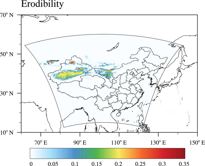
Y. Zeng et al.: WRF-Chem simulations of the East Asian dust storm                                                           2129

2.3.1     BS95                                                    where EIN is collection efficiency from interception, and R
                                                                  is the factor for particle rebound. EIM , EIN , and R are ex-
In the BS95 scheme (Binkowski and Shankar, 1995), Vd is           pressed as
expressed as
                                                                                         2
                                                                                  St
                  1                                               EIM =                          ,                           (13)
Vd = Vg +                    ,                             (5)                 0.8 + St
          Ra + Rs + Ra Rs Vg
where Ra and Rs are aerodynamic and surface resistance; Vg
is the gravitational settling velocity and is given as                     (0.0016 + 0.0061z0 ) dp
                                                                  EIN =                               ,                      (14)
                                                                                   1.414 × 10⁻⁷
        ρp dp2 gCc
Vg =                     ,                                 (6)
           18µ                                                               √
                                                                              St
                                                                  R = e−2          .                                         (15)
where Cc is the Cunningham correction factor as a function
of dp and mean free path of air (λ), and µ is the viscosity       z0 is the roughness length, and dp is particle diameter. The
dynamic of air. The surface resistance is calculated as           Stokes number is given by
              1
Rs =                   ,                                   (7)            ρp dp2
        u∗ (EB + EIM )                                            St =             u.                                        (16)
                                                                          9µdc
where EB is collection efficiency from Brownian diffusion.
EB is calculated as follows:                                      u is the horizontal wind velocity and dc is the diameter of the
              2
                                                                  obstacle.
EB = Sc− 3 ,                                               (8)
                                                                  2.3.3     Z01
where Sc is the Schmidt number, given by Sc = ν/D. ν is
the kinematic viscosity of air, and D is the particle Brownian    In the Z01 scheme (Zhang et al., 2001), the formula of Vd is
diffusivity. EIM is the collection efficiency due to impaction    the same as in the BS95 scheme (Eq. 5). Surface resistance
of the particle with the collecting surface (Gallagher, 2002).    Rs is calculated as
Impaction occurs when there are changes in the direction of
airflow, and particles that cannot follow the flow will collide                       1
                                                                  Rs =                              ,                        (17)
with the obstacle and stay on the surface due to the inertia              0 u∗ (EB + EIM + EIN ) R
(Giardina and Buffa, 2018). EIM is given by
                     3
EIM = 10− St ,                                             (9)    EB = Sc−γ ,                                                (18)
where St is the Stokes number, given by                           where γ depends on land use categories (LUCs) and lies be-
        u2∗ Vg                                                    tween 0.50 and 0.58.
St =             .                                        (10)      EIM is expressed as
         gν
                                                                                       β
St is the ratio of the particle stop distance to the character-                  St
                                                                  EIM =                      ,                               (19)
istic length of the flow and describes the ability of particles                α + St
to adopt the fluid velocity (Pryor et al., 2008; Seinfeld and
Pandis, 2006).                                                    where β equals to 2. α depends on LUC and lies between 0.6
                                                                  and 100.0. The Stokes number is given by
2.3.2     PE92
                                                                  St = Vg u∗ /gA                                             (20)
In PE92 scheme (Peters and Eiden, 1992), the dry deposition
velocity (Vd ) is expressed as                                    over vegetated surfaces (Slinn, 1982) and

                    1                                             St = Vg u2∗ /gν                                            (21)
Vd = Vg +                .                                (11)
                 Ra + Rs
                                                                  over smooth surfaces or surfaces with bluff roughness ele-
The formula of Vg and Ra is the same as in BS95, but the          ments (Giorgi, 1988). EIN is the collection efficiency based
way to calculate Rs is quite different. In PE 92, Rs is param-    on the relative dimensions of the particle to the collector di-
eterized as                                                       ameter (Gallagher, 2002). Interception occurs when particles
                  1                                               moving with the mean flow and the distance between an ob-
Rs =                           ,                          (12)    stacle and particle center is less than half of the diameter.
        u∗ (EB + EIM + EIN ) R

www.geosci-model-dev.net/13/2125/2020/                                                    Geosci. Model Dev., 13, 2125–2147, 2020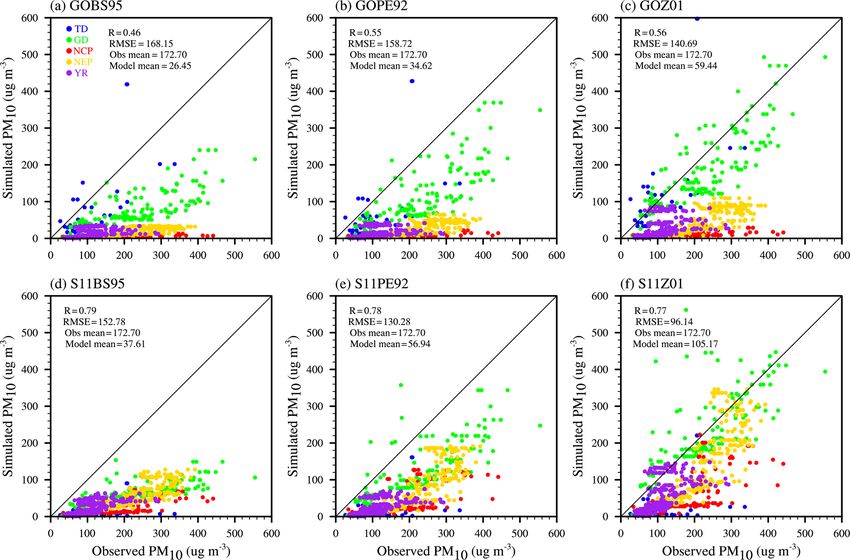
2130                                                     Y. Zeng et al.: WRF-Chem simulations of the East Asian dust storm

Then the particles will collide with and be collected by the        2018). Meteorological conditions are initialized and forced
obstacle. EIN is expressed as                                       at the lateral boundaries using the 6-hourly National Cen-
                                                                    ter for Environmental Prediction Final (NCEP/FNL) Oper-
        1 dp 2

                                                                    ational Global Analysis data at a resolution of 1◦ × 1◦ . For
EIN =                                                       (22)
        2 A                                                         meteorological conditions (such as wind speed and tempera-
                                                                    ture), we reinitialized every 24 h using NCEP/FNL reanaly-
over vegetated surfaces and EIN = 0 for nonvegetated sur-           sis data. For chemistry, the output of the aerosol field (such
faces, where A is the characteristic radius of collectors. A        as the concentration of different aerosol species) from the
depends on LUC and lies between 2.0 and 10.0 mm. R is ex-           previous 1 d run was used as the initial chemical conditions
pressed as                                                          for the next 1 d run. Our simulation period is from 26 April
            √                                                       to 7 May 2017, and one experiment consists of 12 runs,
                St
R = e−1.0            .                                      (23)
                                                                    each of 1 d. In this way, the chemical fields are continuous,
The main differences in formulas used to calculate dry de-          and we can also get more reliable meteorological conditions.
position velocity for three different dry deposition schemes        The MOSAIC aerosol scheme was used for all of the sim-
are listed in Table 2. For Rs , PE92 and Z01 include the col-       ulations. Simulation results prior to 28 April are treated as
lection efficiency from interception (EIN ) and the rebound         model spinup for chemical initial condition and are not in-
effect (R), while these two are neglected in BS95. For the          cluded in results presented in Sect. 3. The model results from
EIM parameterization, all three schemes use St to parame-           1 to 7 May are used for the dust loading and concentration
terize EIM , but the formulas are quite different. BS95 has a       analysis. And the model results from 28 April to 7 May are
different formula from PE92 and Z01, while the PE92 and             used for the dust emission analysis as the dust emissions be-
Z01 have the same formula but with different coefficients.          fore 1 May also have an influence on the dust concentration
For PE92, the coefficient for EIM is constant for all of the sur-   during 1–7 May. To study the dust simulation sensitivity to
face types. For Z01, the coefficients α and β for EIM change        dust emission and dry deposition schemes, we run six experi-
with different surface types. For the EIN parameterization,         ments with two different dust emission schemes and three dry
BS95 ignores this effect; PE92 and Z01 use different for-           deposition schemes (See Table 3). The corresponding model
mulas and variables to calculate EIN . When large particles         configuration for dry deposition processes of the six exper-
(usually > 5 µm) hit the nonsticky surface, they are liable to      iments also listed in Table 3. We note here that the USGS
rebound from the surface if they have sufficient kinetic en-        LUCs should be selected for the Z01 dry deposition scheme.
ergy. The rebound factor R represents the fraction of parti-
cles that stick to the surface (Seinfeld and Pandis, 2006). For     2.5     Measurements
rebound effect, BS95 does not consider
                                   √       it; PE92 and Z01 use
the same e-exponential form e−b St to calculate the rebound         2.5.1    PM10
effect with a different coefficient b. For PE92, b is 2.0; for
Z01, b is 1.0. In addition, the parameterization of St is quite     Hourly surface observed PM10 is used to compare with the
different for different dry deposition schemes. For BS95, the       simulated PM10 from WRF-Chem. In China, hourly sur-
formulation of St tends to emphasize the nature of the flow         face PM10 concentrations were collected from more than
field (Binkowski and Shankar, 1995; Pryor et al., 2008). For        1000 environmental monitoring stations (locations shown
Z01, the formulation of St is from Slinn (1982) over vege-          in results section) maintained by the Ministry of Environ-
tated surfaces and from Binkowski and Shankar (1995) over           mental Protection (MEP). The hourly PM10 data from 1 to
smooth surfaces. The formulation of St from Slinn (1982)            7 May 2017 were downloaded from https://quotsoft.net/air/
and Peters and Eiden (1992) are focus on the individual ob-         (last access: 3 April 2020). We colocated the PM10 data with
stacles (Pryor et al., 2008).                                       WRF-Chem simulation grids to evaluate model performance
                                                                    with different configurations.
2.4    Experiments design
                                                                    2.5.2    MODIS AOD
We use WRF-Chem v3.9 with 20 km × 20 km horizontal res-
olution and 35 vertical levels with model top pressure at           Daily aerosol optical depth (AOD) from the Moderate Res-
50 hPa. The domain covers most of East Asia (14–60◦ N, 74–          olution Imaging Spectroradiometer (MODIS) is used to
130◦ E) as shown in Fig. 1. The simulation period is from           compare with our simulated AOD from WRF-Chem. The
26 April to 7 May 2017 with time step of 60 s and fre-              MODIS on board the Aqua satellite was launched by the
quency of output every hour. The time step between radia-           NASA in 2002, and Aqua is a part of the A-Train satellite
tion physics calls is 20 min. During this period, a severe dust     constellation. To compare modeled AOD with observations,
storm event originated from northwestern China and Outer            we use AOD retrievals at 550 nm from MODIS AOD prod-
Mongolia, and air quality deteriorated dramatically in a very       ucts on Aqua with daily gridded data at a resolution of 1◦ ×1◦
short time in downwind areas (Guo et al., 2019; Zhang et al.,       (MYD08_D3, Collection 6, combined dark target and deep

Geosci. Model Dev., 13, 2125–2147, 2020                                              www.geosci-model-dev.net/13/2125/2020/
Y. Zeng et al.: WRF-Chem simulations of the East Asian dust storm                                                                  2131

Table 2. Three dry deposition schemes.

                  Scheme     BS95                         PE92                            Z01

                  Vd                         1
                             Vd = Vg + R +R +R                         1
                                                          Vd = Vg + R +R                                  1
                                                                                          Vd = Vg + R +R +R
                                        a  s   a Rs Vg               a   s                           a  s   a Rs V g

                  Rs         Rs = u (E 1+E )              Rs = u (E +E1 +E )R             Rs = ε u (E +E1 +E )R
                                   ∗ B    IM                    ∗ B    IM  IN                   0 ∗ B    IM IN
                                                                       2                            β
                  EIM        EIM = 10−St                            St
                                                          EIM = 0.8+St                    EIM = α+StSt

                                                                                                   2
                                                                (0.0016+0.0061z0 )dp               d
                  EIN                                     EIN =                           EIN = 12 Ap
                                                                     1.414×10⁻⁷
                                                                 √                               √
                  R          1.0                          R = e−2 St                      R = e− St
                                    u2 V
                                  ∗ g                            ρp d 2                         V u
                  St         St = gν                      St = 9µdp u                          g ∗
                                                                                          St = gA  (vegetated surfaces)
                                                                  c

                                                                                                V u2
                                                                                               g ∗
                                                                                          St = gν  (smooth surfaces)

Table 3. Model experiments and the corresponding model configu-           60 m and 1 km, respectively. We use the CALIPSO level 2
ration in WRF-Chem.                                                       APro product (V4.20) to obtain the aerosol extinction co-
                                                                          efficient (CAL_LID_L2_05kmAPro-Standard-V4-20). The
   Experiment     Dust emission     Dry deposition   aer_dry-             CALIPSO data are available at https://www-calipso.larc.
   name           scheme            scheme           dep_opt              nasa.gov/ (last access: 23 April 2020).
   GOBS95         GOCART            BS95                   1
   GOPE92         GOCART            PE92                 101
   GOZ01          GOCART            Z01                  301              3     Results
   S11BS95        Shao2011          BS95                   1
   S11PE92        Shao2011          PE92                 101              3.1    Meteorological conditions
   S11Z01         Shao2011          Z01                  301
                                                                          Dust emission and transport processes are closely related
                                                                          to the meteorological conditions. So we first evaluated the
blue AOD). The MODIS Aqua collection daily MYD08_D3                       model performance in simulating the synoptic conditions.
files were obtained from https://ladsweb.nascom.nasa.gov                  Figure 2 shows the surface meteorological conditions dur-
(last access: 23 April 2020). As Aqua passes through ev-                  ing the dust event. Figure 2a, d, g, and j show the daily
ery region of Earth at around 13:30 local time, we extract                mean wind field at 10 m and daily mean temperature at 2 m
the model simulation results at 13:00 to compare with the                 from NCEP/FNL reanalysis data. The meteorological con-
daily MODIS AOD. For the model results, first we divided                  ditions at 700 hPa are shown in the Supplement (Fig. S1).
the domain into different time zones according to the lon-                This dust storm was triggered by the development of a Mon-
gitude. Then the model results at corresponding UTC when                  golian cyclone (Figs. S1c and 2d). With the strong north-
the local time is 13:00 are extracted. The colocated model                west and southwest wind near the dust source region, emitted
AOD results for each day are used in comparison with daily                dust was transported to the southeast and northeast of China
MODIS AOD.                                                                (Figs. S1c, e and 2d, g). Figure 2b, e, h, and k show the WRF-
                                                                          Chem-simulated daily mean wind field at 10 m and daily
2.5.3   CALIPSO data                                                      mean temperature field at 2 m. Figure. 2c, f, i, and l show
                                                                          the difference in daily mean wind speed at 10 m between
The vertical profile of aerosol extinction coefficient at a               WRF-Chem simulation and NCEP/FNL reanalysis data. The
wavelength of 532 nm from the Cloud-Aerosol Lidar and In-                 WRF-Chem model was able to simulate the wind speed well
frared Pathfinder Satellite observation (CALIPSO) satellite               over the dust source regions (the Taklimakan Desert and the
is used to evaluate model results. The CALIPSO launched                   Gobi Desert) and eastern and southern China, where the dif-
on 28 April 2006 equipped with CALIOP (Cloud-Aerosol                      ferences were mostly in the range of −2.0–2.0 m s−1 . The
Lidar with Orthogonal Polarization). The CALIOP lidar pro-                wind speed is slightly underestimated near the center of the
vides an along-track observation of aerosol and cloud vertical            cyclone (Fig. 2c, f, i, l) and as this is away from dust source
profile. The vertical and horizontal resolutions for CALIOP               regions, we do not expect this underestimation causes large
from the surface to 8.2 km are 30 and 333 m, respectively.                bias in dust emissions. The correlation coefficient (R) and
Above 8.2 km, the vertical and horizontal resolutions are                 root mean square error (RMSE) between WRF-Chem sim-

www.geosci-model-dev.net/13/2125/2020/                                                      Geosci. Model Dev., 13, 2125–2147, 2020
2132 Y. Zeng et al.: WRF-Chem simulations of the East Asian dust storm
ulation and FNL reanalysis data for temperature at 2 m, U Inner Mongolia and the south of Outer Mongolia (Fig. 5e).
component of wind, V component of wind, and wind speed This is consistent with Fig. 5g. When the friction velocity
at 10 m during simulation period are shown in Table 4. The R is larger than threshold friction velocity, dust can be emit-
for time-averaged temperature at 2 m, U component of wind, ted from the surface. Figure 5b, d, f, and h show the spa-
V component of wind, and wind speed at 10 m from 1 to tial distribution of wind speed at 10 m, threshold velocity, the
7 May are 1.0, 0.90, 0.86, and 0.82, respectively. The RMSE difference between wind speed at 10 m and threshold veloc-
for time-averaged temperature at 2 m, U component of wind, ity, and the dust emission flux from the GOCART dust emis-
V component of wind, and wind speed at 10 m from 1 to sion scheme. Different from Shao2011, the dust emission re-
7 May are 1.03, 1.08, 0.98, and 1.11, respectively. The R for gions from GOCART are not only determined by wind speed
temperature, U component of wind, V component of wind, but also constrained by the erodibility factor (Eq. 1). From
and wind speed at 700 hPa from 1 to 7 May are 1.0, 0.94, Fig. 5f, the threshold velocity is much smaller than the wind
0.91, and 0.95, respectively (Table S1 in the Supplement). speed at 10 m in most areas. In these areas, GOCART uses
The RMSE for temperature, U component of wind, V com- Eq. (1) to calculate the dust emission flux, and the source
ponent of wind, and wind speed at 700 hPa from 1 to 7 May function S depends on the erodibility factor. The dust emis-
are 0.67, 2.34, 2.70, and 1.76, respectively (Table S1). Over- sion flux in GOCART is directly scaled by erodibility fac-
all, the correlation coefficients are generally large, and the tor. Figure 1 shows the erodibility factor, which describes the
RMSEs are generally small. This indicates that WRF-Chem fraction of erodible surface in each grid cell. As shown in
performed well in simulating the meteorological conditions. Fig. 5h, dust emission occurs where the wind speed is high
We also compared the difference in the meteorological con- and the erodibility factor is larger than 0.
ditions in our six experiments and found that the difference Over the TD, Shao2011 produces lower dust emission flux
is negligible (Fig. S2 and Table S2). than GOCART. One reason may be the formula used to cal-
culate the threshold velocity (Eq. 3). The formula used to
3.2 Dust simulation sensitivity to dust emission calculate threshold velocity is from Marticorena and Berga-
schemes metti (1995), which was originally designed to calculate
threshold friction velocity (see LeGrand et al., 2019 for de-
In this section, we examine the changes in the simulated tails). This inconsistency leads to a very small threshold ve-
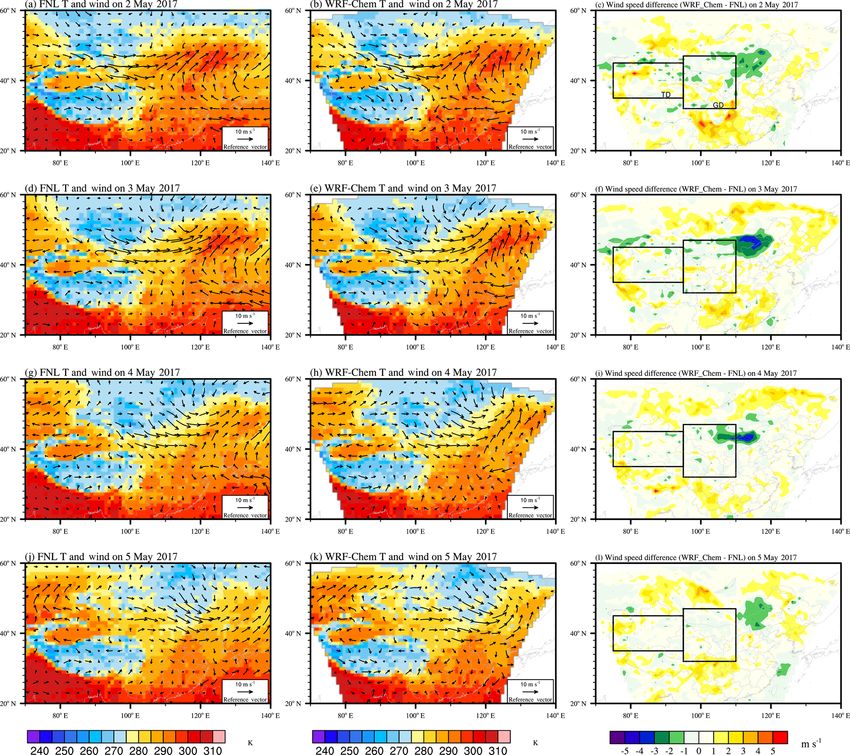
dust loading using different dust emission schemes. Figure 3 locity in GOCART, which may result in dust emission at low
shows simulated mean dust loading for six experiments over wind speed. Another reason may be the incorrect soil parti-
the 7 d simulation period 1–7 May 2017. When using the cle size distribution over the TD (Wu and Lin, 2014). The
same dry deposition scheme (BS95, PE92, or Z01), different incorrect soil particle size distribution can lead to the unrea-
dust emission schemes give very different dust spatial dis- sonable dust emission flux in Shao2011 over the TD. Over
tributions. Compared with the Shao2011 scheme, GOCART the GD, the GOCART scheme has lower dust emission than
has higher dust loading over the Taklimakan desert (TD) the Shao2011 scheme. As mentioned by Su and Fung (2015),
but has relatively lower dust loading over the Gobi Desert the erodibility factor over the GD is highly underestimated
(GD), the south of Outer Mongolia, and most parts of north- and needs to be improved for the GOCART dust emission
ern China. The difference in the spatial distribution of dust scheme.
loading is mainly caused by the different spatial distributions As we mentioned in Sect. 2.2.2, Shao2011 used in this
of dust emission flux from dust emission schemes, as shown study is based on WRF-Chem v3.9 with some modifi-
in Fig. 4. As the dust emissions before 1 May also have an cations from WRF-Chem v3.7.1. The modified Shao2011
influence on the dust loading during 1–7 May, the total dust simulates better dust loading than the original Shao2011
emissions from 28 April to 7 May are analyzed. The total scheme in WRF-Chem v3.9 (not shown). Simulated dust
dust emissions from 00:00 UTC on 28 April to 23:00 UTC on emission fluxes are quite different when using two versions
7 May over the GD from GOCART and Shao2011 are 4.90 of the Shao2011 scheme in WRF-Chem v3.9 and WRF-
and 13.88 Tg, respectively. The total dust emissions from Chem v3.7.1, which is mainly caused by different soil par-
00:00 UTC on 28 April to 23:00 UTC on 7 May over the TD ticle size distributions in two versions. The differences in
from GOCART and Shao2011 are 7.16 and 2.75 Tg, respec- Shao2011 among different WRF-Chem versions are docu-
tively. Over the GD, the Shao2011 scheme has higher dust mented in Appendix B.
emission than GOCART, while over the TD, the GOCART
scheme has higher dust emission than Shao2011 (Fig. 4c). 3.3 Dust simulation sensitivity to dry deposition
Figure 5a, c, e, and g show the spatial distribution of fric- schemes
tion velocity, threshold friction velocity, the difference be-
tween friction velocity and threshold friction velocity, and In this section, we analyze dust simulation sensitivity to dif-
the dust emission flux from Shao2011 at 06:00 UTC on ferent dry deposition schemes using the six experiments. For
3 May. The areas where the friction velocity is greater than simulated dust loading using the GOCART dust emission
the threshold friction velocity is mainly located in the west of scheme (Fig. 3a–c), compared to the BS95 dry deposition
Geosci. Model Dev., 13, 2125–2147, 2020 www.geosci-model-dev.net/13/2125/2020/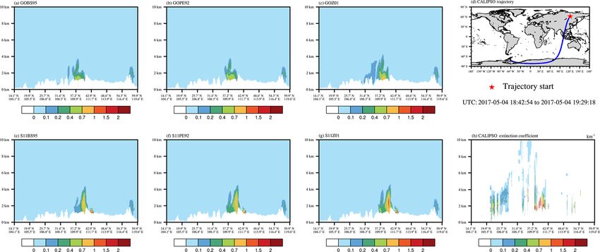
Y. Zeng et al.: WRF-Chem simulations of the East Asian dust storm                                                              2133

Table 4. Correlation coefficient (R) and root mean square error (RMSE) between WRF-Chem simulation and FNL reanalysis data for daily
mean temperature at 2 m, U component of wind, V component of wind, and wind speed at 10 m during the dust event time period over the
whole domain. The last two rows show the R and RMSE for the time-averaged temperature at 2 m, U component of wind, V component of
wind, and wind speed at 10 m from 1 to 7 May.

                                Day           R/RMSE      Temperature      U       V    Wind speed
                                1 May         R                   0.99   0.86   0.85           0.75
                                1 May         RMSE                1.32   1.51   1.59           1.60
                                2 May         R                   0.99   0.90   0.88           0.82
                                2 May         RMSE                1.28   1.61   1.60           1.70
                                3 May         R                    1.0   0.91   0.90           0.84
                                3 May         RMSE                1.22   1.60   1.64           1.76
                                4 May         R                   0.99   0.87   0.87           0.78
                                4 May         RMSE                1.35   1.57   1.49           1.63
                                5 May         R                   0.99   0.88   0.87           0.80
                                5 May         RMSE                1.23   1.49   1.44           1.57
                                6 May         R                   0.99   0.88   0.87           0.80
                                6 May         RMSE                1.32   1.56   1.52           1.63
                                7 May         R                   0.99   0.89   0.82           0.79
                                7 May         RMSE                1.37   1.42   1.30           1.39
                                1 to 7 May    R                    1.0   0.90   0.86           0.82
                                1 to 7 May    RMSE                1.03   1.08   0.98           1.11

scheme, PE92 and Z01 produce higher dust loading over                  The surface collection efficiency is comprised of Brow-
the dust source regions and remote regions. The relative dif-       nian diffusion, impaction, and interception and is corrected
ferences in mean dust loading from PE92 and Z01 relative            for particle rebound (see Eq. 12). Collection from Brownian
to BS95 are 20 % and 59 %, respectively. As for the simu-           diffusion is most important for the smaller particles, while
lated dust loading using the Shao2011 dust emission scheme          collection from impaction and interception play a more im-
(Fig. 3d–f), PE92 and Z01 schemes also produce higher dust          portant role for large particles in surface collection processes.
loading than the BS95 scheme, and the differences relative          Figure 6c shows the surface collection efficiency from im-
to BS95 are 72 % and 116 %, respectively. This indicates that       paction (EIM ) from different schemes as a function of parti-
dust simulation is very sensitive to dry deposition schemes.        cle diameter. BS95 gives the largest EIM , and Z01 gives the
   Figure 6a shows the modeled dry deposition velocity over         smallest. Based on field observation data, Slinn (1982) used a
desert surface. As desert dust mass is mainly concentrated          semiempirical fit for smooth surface (Eq. 9), and Binkowski
in the large particle size range, our dry deposition analysis       and Shankar (1995) adopted this formula for EIM and used
focuses on the coarse mode (2.5–10 µm) (Kok, 2011; Zhao             it for all land surface types. Peters and Eiden (1992) uses
et al., 2013). The reference diameter of the coarse mode            Eq. (19) to describe EIM , with α equals 0.8, and β equals
is defined at 5 µm (Fig. 6). BS95 produces larger Vd than           2 to get the best fit for the data collected over a spruce for-
PE92 and Z01 in the coarse aerosol mode. Larger Vd leads            est (Eq. 13). In Zhang et al. (2001) scheme, α varies with
to larger dry deposition and thus lower dust loading, consis-       LUC, and β is chosen as 2 (Eq. 19). For BS95 and PE92,
tent with the lower simulated dust loading from the BS95            the formula of EIM is derived from a specific land surface
scheme discussed above (Fig. 3). In Eq. (5), the dry deposi-        type, but they have been applied to all land surface types in
tion velocity is comprised of gravitational velocity, aerody-       WRF-Chem. This may lead to large uncertainties for dry de-
namic resistance, and surface resistance. The diversity of dif-     position over the whole domain with different surface types.
ferent dry deposition schemes mainly comes from the way to          As the EIM of Z01 varies with LUC, Z01 may have a better
parameterize surface resistance, and differences from gravi-        physical treatment of EIM than the other two dry deposition
tational settling and aerodynamics resistance are small (not        schemes.
shown), consistent with previous studies (e.g., Bergametti et          Figure 6d shows the surface collection efficiency from in-
al., 2018). Figure 6b shows the surface resistance from dif-        terception (EIN ). EIN depends on the particle diameter and
ferent schemes as a function of particle diameter (dp ). In the     the characteristic radius of the collectors (Seinfeld and Pan-
coarse aerosol mode, Z01 produces the largest surface resis-        dis, 2006). EIN is important for large particles on hairs at
tance, followed by PE92 and BS95. Larger surface resistance         the leaf surface and is negligible over nonvegetated surfaces
causes smaller dry deposition velocity in Z01, thus larger          such as the desert surface we analyzed here (Chamberlain,
dust concentration as shown in Fig. 3.                              1967; Slinn, 1982; Zhang et al., 2001). In BS95, the effect of

www.geosci-model-dev.net/13/2125/2020/                                                 Geosci. Model Dev., 13, 2125–2147, 2020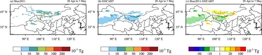
2134                                                      Y. Zeng et al.: WRF-Chem simulations of the East Asian dust storm

Figure 2. The left two columns show the surface meteorological conditions during the dust event. The color contours show the daily mean
temperature field at 2 m. Vectors represent the daily mean wind field at 10 m. Panels (a), (d), (g), and (j) show the NCEP/FNL reanalysis
data. Panels (b), (e), (h), and (k) show the WRF-Chem simulation. The rightmost column shows the difference in daily mean wind speed at
10 m between WRF-Chem simulation and NCEP/FNL reanalysis data. The rectangles show the dust source regions. “TD” is the Taklimakan
Desert. “GD” is the Gobi Desert.

                                                                                          √
interception is not considered. In the original PE92 scheme            effect as R = e−b St suggested by Slinn (1982) (Zhang and
as described in Peters and Eiden (1992), EIN is also not con-          Shao, 2014; Zhang et al., 2001), while some dry deposi-
sidered. But in the PE92 scheme used in WRF-Chem, EIN                  tion schemes do not include the rebound effect with R = 1.0
increases with particle diameter as in Eq. (14). In Z01, the           (Binkowski and Shankar, 1995; Petroff and Zhang, 2010;
effect of interception is considered as Eq. (22) over vege-            Zhang and He, 2014). BS95 does not consider the rebound
tated surface and is not considered for nonvegetated surface           effect. b is equal to 2.0 for the PE92 scheme and 1.0 for the
(as shown in Fig. 6d over desert surface type). The parame-            Z01 scheme. Another difference between PE92 and Z01 is
terization of EIN partially results in the difference in surface       the threshold particle diameter for including the rebound ef-
resistance between PE92 and the other two dry deposition               fect. Rebound effect is included for PE92 when particles are
schemes.                                                               larger than 0.625 µm and for Z01 when particles are larger
   Figure 6e shows the rebound factor from different dry de-           than 2.5 µm. In summary, the smaller EIM and rebound fac-
position schemes. Rebound and resuspension have long been              tor lead to larger Rs in Z01, while the larger EIM leads to
recognized as a mechanism by which the surface can act                 smaller Rs in BS95, and the moderate EIM and rebound ef-
as sources of particles (Pryor et al., 2008). Due to limited           fect give a moderate Rs for PE92.
knowledge of particle rebound and resuspension processes,                 Figure 6f shows the Stokes number from different dry de-
most dry deposition models adopted the form of the rebound             position schemes. Over smooth surfaces, the formula of St

Geosci. Model Dev., 13, 2125–2147, 2020                                                  www.geosci-model-dev.net/13/2125/2020/
Y. Zeng et al.: WRF-Chem simulations of the East Asian dust storm 2135 Figure 3. Spatial distribution of simulated mean dust loading for six experiments (a) GOBS95, (b) GOPE92, (c) GOZ01, (d) S11BS95, (e) S11PE92, and (f) S11Z01 over the 7 d simulation period from 00:00 UTC on 1 May to 23:00 UTC on 7 May 2017 (unit: mg m−2 ). Figure 4. The simulated total dust emission (10−3 Tg) from two dust emission schemes: (a) Shao2011 and (b) GOCART from 00:00 UTC on 28 April to 23:00 UTC on 7 May 2017. (c) The total dust emission flux difference between Shao2011 and GOCART. The diameter of the emitted dust is less than 10 µm in both GOCART and Shao2011 dust emission schemes. for BS95 and Z01 is the same, as shown in Eq. (10). In PE92, is most suitable for operational use in the size range 0.2– St is calculated using Eq. (16), which is similar to the for- 10 µm. All of these indicate that the Z01 dry deposition mula used in Slinn (1982). BS95 and Z01 schemes give a scheme is more physically meaningful than other two dry de- larger St than PE92. The Stokes number is used to calculate position schemes. both R and EIM . The difference in Stokes numbers and the different formulas of R and EIM lead to the different R and 3.4 Comparisons with observations EIM among different dry deposition schemes (Fig. 6c and e). Our discussion indicates that Z01 has a better physical To better evaluate the performance of different experiments, treatment of dry deposition velocity, as Z01 considers the re- we compared the model results with observations. Figure 7 bound effect, and EIM changes with LUC. The Z01 scheme shows hourly observed PM10 concentrations over obser- has also been documented to agree better with measured dry vational sites at 02:00 UTC on 4 May 2017 (10:00 Bei- deposition fluxes and dry deposition velocity (e.g., Zhang et jing Time, BJT, on 4 May 2017). Very high PM10 values al., 2012; Connan et al., 2018). Zhang et al. (2012) compared (> 1000 µg m−3 ) are observed in northern China. Figure 8 the dry deposition fluxes measured at five sites in Taiwan compares simulated PM10 in six experiments with observed with the modeled dry deposition fluxes and found that the PM10 . During the comparison, the observational sites closest measured dry deposition fluxes can be reproduced reason- to the model grids are paired up. The correlation coefficients ably well using the Z01 scheme. Connan et al. (2018) con- (R), root mean square errors (RMSE) between model and ducted experimental campaigns on-site to determine dry de- observations, and the mean simulated and observed PM10 position velocity of aerosols and found that the Z01 scheme for all of the sites over the five regions during the 7 d pe- www.geosci-model-dev.net/13/2125/2020/ Geosci. Model Dev., 13, 2125–2147, 2020
2136                                                         Y. Zeng et al.: WRF-Chem simulations of the East Asian dust storm

Figure 5. Spatial distributions of (a) friction velocity (u∗ ), (c) threshold friction velocity (u∗t ), and (e) the difference between u∗ and u∗t
(u∗ − u∗t ) from Shao2011 dust emission scheme at 06:00 UTC on 3 May 2017; (b) wind speed at 10 m (u10 ), (d) threshold velocity (ut ), and
the difference between u10 and ut (u10 − ut ) from the GOCART dust emission scheme at 06:00 UTC on 3 May 2017. Spatial distribution of
(g) dust emission flux from Shao2011 and (h) dust emission flux from GOCART at 06:00 UTC on 3 May 2017.

riod 1–7 May are marked in Fig. 8. The simulated PM10                      periments. For other regions (North China Plain, NCP, North-
of all of the six experiments have obviously underestimated                east Plain, NEP, and the middle and lower reaches of the
the observations. Among all of these experiments, GOBS95                   Yangtze River plain, YR), S11Z01 gives a relatively larger R
has the lowest average PM10 concentration, with a value of                 and smallest RMSE. For all of the stations in total, S11Z01
26.45 µg m−3 , and S11Z01 has the largest one, with a value                gives a larger R of 0.83 and the smallest RMSE of 82.98.
of 105.17 µg m−3 , the closest one to the observed mean value              Overall, the S11Z01 experiment has the best performance for
of 172.70 µg m−3 . S11Z01 gives a large R of 0.77 and the                  simulating this dust storm.
smallest RMSE of 96.14 compared to other experiments. Ta-                     Figure 9 shows the MODIS-observed daily mean AOD
ble 5 shows the R and RMSE between the model and ob-                       and WRF-Chem-simulated AOD over the simulation period
servations for PM10 for six experiments over five subregions               1–5 May. For strong dust storms like the one we examined
and over the whole of China. Over the TD, GOBS95 gives                     here, dust particles contribute the most to AOD, and AOD
the largest R and smallest RMSE. Over the GD, GOZ01 and                    therefore can represent the dust loading in the atmosphere. To
S11Z01 give a better performance compared with other ex-                   match the MODIS AOD observation time, simulated AOD

Geosci. Model Dev., 13, 2125–2147, 2020                                                        www.geosci-model-dev.net/13/2125/2020/
Y. Zeng et al.: WRF-Chem simulations of the East Asian dust storm                                                                         2137

Figure 6. (a) Dry deposition velocity (Vd ), (b) surface resistance (Rs ), (c) surface collection efficiency from impaction (EIM ), (d) surface
collection efficiency from interception (EIN ), (e) rebound (R), and (f) Stokes number (St) as a function of particle diameter (dp ) over desert
surface computed using different dry deposition schemes (BS95, PE92, and Z01). The colored dots indicate values at the reference diameter
of 5 µm.

Figure 7. Five subregions and observed PM10 concentrations. Key: “1” represents the Taklimakan Desert (TD), “2” represents the Gobi
Desert (GD), “3” represents the Northeast Plain (NEP), “4” represents the North China Plain (NCP), and “5” represents the middle and lower
reaches of Yangtze River plain (YR). The colored dots represent observed PM10 concentrations over observational sites at 02:00 UTC on
4 May 2017 (10:00 Beijing Time, BJT, on 4 May 2017).

www.geosci-model-dev.net/13/2125/2020/                                                         Geosci. Model Dev., 13, 2125–2147, 2020
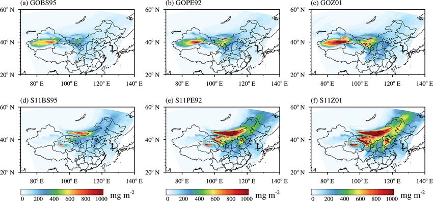
2138                                                        Y. Zeng et al.: WRF-Chem simulations of the East Asian dust storm

Figure 8. Simulated PM10 versus observed PM10 for six experiments (a) GOBS95, (b) GOPE92, (c) GOZ01, (d) S11BS95, (e) S11PE92,
and (f) S11Z01 over the 7 d simulation period 1–7 May 2017. “Obs mean” is mean PM10 over 1–7 May from observation; “Model mean”
is mean PM10 over 1–7 May from simulation; “R” is the correlation coefficient between model and observations; “RMSE” is the root mean
square error. Different color dots represent different regions as shown in Fig. 6.

Figure 9. Simulated and observed mean AOD over the simulation period 1–5 May. Panels (a)–(e) show the distribution of daily mean aerosol
optical depth (AOD) at 550 nm derived from MODIS-Aqua. Panels (f)–(j) show the WRF-Chem-simulated AOD for the GOBS95 experiment.
Panels (k)–(n) show the WRF-Chem-simulated AOD for the S11Z01 experiment. The model results are extracted from the simulation results
at 13:00 local time for each region to match the MODIS observation time (for details see Sect. 2.5). All of the other experiments and for the
period 1–6 May are shown in Fig. S1. Grid points without valid MODIS AOD retrieval are masked for both observational and model results.

at 13:00 local time is used for comparison (see Sect. 2.5                and model results in Fig. 9. A major dust emission event
for details). For each 1◦ × 1◦ grid with observed AOD from               occurred over the GD on 3 May (Fig. 9c). Shao2011 sim-
MODIS, the average value of simulated AOD from WRF-                      ulated well the dust emission event over the GD on 3 May
Chem in this grid is calculated. Grid points without valid               (Fig. 9m), while GOCART obviously underestimated dust
MODIS AOD retrieval are masked for both observational                    emission over the GD (Fig. 9h). On 4 May, emitted dust from

Geosci. Model Dev., 13, 2125–2147, 2020                                                     www.geosci-model-dev.net/13/2125/2020/
Y. Zeng et al.: WRF-Chem simulations of the East Asian dust storm                                                                 2139

Table 5. Correlation coefficient (R) and root mean square error (RMSE) between the model and observations for PM10 over five subregions
and for all of the stations over whole China in Fig. 7 for six experiments listed in Table 3.

                      Region    R/RMSE       GOBS95      GOPE92      GOZ01      S11BS95     S11PE92      S11Z01
                      TD        R                0.64        0.53       0.59        0.34         0.37       0.37
                      TD        RMSE            79.61       91.91     106.61      124.25       119.54     115.68
                      GD        R                0.75        0.78       0.82        0.76         0.75       0.74
                      GD        RMSE           174.81      137.14      77.81      193.23       128.21      82.58
                      NCP       R                0.75        0.73       0.73        0.78         0.76       0.77
                      NCP       RMSE            231.2      221.05     197.43      189.08       164.25     107.20
                      NEP       R                0.62        0.63       0.58        0.70         0.68       0.68
                      NEP       RMSE           177.17      174.52     171.96      159.47       144.77     126.91
                      YR        R                0.45        0.42       0.43        0.67         0.61       0.61
                      YR        RMSE           105.96      105.97      93.97       94.07        93.79      69.94
                      Total     R                0.50        0.60       0.63        0.85         0.83       0.83
                      Total     RMSE           146.58      137.96     120.57      133.71       113.88      82.98

the GD was transported to northeast China, and the highest            in simulating this dust storm. As we discussed in Sect. 3.2,
AOD values for this case study were observed in northern              the Z01 dry deposition scheme indeed has a better physical
China (Fig. 9d). As the GD is the main dust source region             treatment and performs better than some other dry deposition
of this dust storm, Shao2011 correctly captured the emis-             schemes.
sion phase of this dust event. Simulated AOD values from
the S11Z01 configuration produced the closest match to the
observed daily MODIS AOD with respect to the magnitude                4   Summary and discussion
and spatial pattern (Figs. 9n and S3). For a more quantitative
comparison, Table 6 shows the correlation coefficient (R)             In this study, we analyzed the dust simulation sensitivity to
and root mean square error (RMSE) between the model and               different dust emission schemes and dry deposition schemes.
observed AOD for six experiments during 1–7 May. Overall,             In order to compare different dust emission schemes, the
the S11Z01 experiment gives a larger correlation coefficient,         Shao2011 dust emission scheme has been implemented into
and the RMSE is almost the same among different experi-               the MOSAIC aerosol scheme in WRF-Chem v3.9. Six model
ments; the correlation coefficient is still lower than 0.5. The       experiments were conducted to simulate the dust storm in
low correlation may partly come from the spatial and tem-             May 2017 over East Asia, with two dust emission schemes
poral limitation of satellites and the difficulties to retrieve       (GOCART and Shao2011) and three dry deposition schemes
aerosol in the vicinity of clouds for satellites.                     (BS95, PE92, and Z01). The simulation results of different
   To evaluate the model performance in simulating the ver-           experiments were evaluated against surface and satellite ob-
tical profile of dust aerosol, we compared the extinction co-         servations.
efficient from the model and from CALIPSO (Fig. 10). Fig-                Our results show that dust loading is very sensitive to dif-
ure 10 shows the simulated and observed aerosol extinction            ferent dry deposition schemes. The relative difference in dust
profiles at 532 nm at 18:00 UTC on 4 May. The trajectory              loading in different experiments range from 20 % to 116 %
of CALIPSO passes East Asia (Fig. 10d). All of the six ex-            when using different dry deposition schemes. The difference
periments show the similar dust location in the atmosphere,           in dry deposition velocity in different dry deposition schemes
which is consistent with the CALIPSO observation. How-                comes from the parameterization of surface resistance, and
ever, the magnitude of dust concentration differs substan-            difference in surface resistance mainly comes from the pa-
tially. The simulated extinction coefficients using GOCART            rameterization of collection efficiency from impaction and
dust emission schemes are significantly underestimated com-           rebound effect. In addition, different dust emission schemes
pared to the CALIPSO observation (Fig. 10a, b, and c),                result in different spatial distributions of dust loading, as dust
while the modeled extinction coefficients using Shao2011              emission fluxes in dust source regions differ substantially
dust emission scheme agrees better with observation though            among different dust emission schemes, which is mainly at-
they are still underestimated (Fig. 10e, f and g). Among all of       tributed to differences in the threshold conditions for dust
the six experiments, results from S11Z01 agree the best with          emission and in formulas and parameters for calculating
observation.                                                          dust emission flux. We noted that the Shao2011 dust emis-
   In summary, both ground and satellite observations indi-           sion scheme is different among different WRF-Chem ver-
cate that the S11Z01 experiment yields the best performance           sions, and a significant difference exists in the simulated dust
                                                                      emission fluxes between WRF-Chem v3.9 and WRF-Chem

www.geosci-model-dev.net/13/2125/2020/                                                   Geosci. Model Dev., 13, 2125–2147, 2020
You can also read