A Comparison of Graph Optimization Approaches for Pose Estimation in SLAM
←
→
Page content transcription
If your browser does not render page correctly, please read the page content below
A Comparison of Graph Optimization
        Approaches for Pose Estimation in SLAM
                              And̄ela Jurić∗,1 , Filip Kendeš∗ , Ivan Marković∗ , Ivan Petrović∗
          ∗   University of Zagreb, Faculty of Electrical Engineering and Computing, Zagreb, Croatia
                          {andela.juric, filip.kendes, ivan.markovic, ivan.petrovic}@fer.hr

       INTEL                     MIT                    M3500                   M3500a                  M3500b                   M3500c

      Sphere-a                   Torus                   Cube                    Garage                  Cubicle                     Rim

              Fig. 1: Two-dimensional (first row) and three-dimensional (second row) pose graphs used in the benchmarking process.

   Abstract—Simultaneous localization and mapping                         between new observations and the map using correspon-
(SLAM) is an important tool that enables autonomous                       dences based on sensor data. The second part computes
navigation of mobile robots through unknown environments.                 the robot poses and the map given the constraints. It
As the name SLAM suggests, it is important to obtain a
correct representation of the environment and estimate a                  can be divided into graph and smoothing methods. An
correct trajectory of the robot poses in the map. Dominant                example of a current state-of-the-art optimization-based
state-of-the-art approaches solve the pose estimation                     method is g2 o [2]. It is a general optimization framework
problem using graph optimization techniques based on                      for nonlinear least squares
the least squares minimization method. Among the most                                                √ problems. One of the first
                                                                          smoothing approaches, SAM, was presented in [3].
popular approaches are libraries such as g2 o, Ceres,
GTSAM and SE-Sync. The aim of this paper is to describe                   An improvement to this method, incremental smoothing
these approaches in a unified manner and to evaluate them                 and mapping
                                                                                √        (iSAM), was introduced in [4]. iSAM ex-
on an array of publicly available synthetic and real-world                tends SAM to provide an efficient solution to the full
pose graph datasets. In the evaluation experiments, the                   SLAM problem by updating the factorization of the sparse
computation time and the value of the objective function of               smoothing information matrix. The upgrade of iSAM,
the four optimization libraries are analyzed.
   Index Terms—pose-graph, optimization, trajectory esti-                 iSAM2, is presented in [5]. These smoothing methods
mation, SLAM, g2 o, GTSAM, Ceres, SE-Sync                                 are implemented in GTSAM [6], which is another state-
                                                                          of-the-art optimization library.
                    I. I NTRODUCTION                                         An elegant example of a SLAM problem is the so-
    After years of dominance in the SLAM scene,                           called pose SLAM, which avoids building an explicit
filter-based methods are more and more replaced by                        map of the environment. The objective of pose SLAM
optimization-based approaches. Pose graph optimization                    is to estimate the trajectory of the robot given the
(PGO) was first introduced in [1], but was not very                       loop closing and odometric constraints. These relative
popular due to computational inefficiency. Today, with                    pose measurements are usually obtained from IMU, laser
the increase of the computational power, PGO methods                      sensor, cameras or wheel odometry using ego-motion
have become the state-of-the-art and are able to solve                    estimation, scan matching, iterative closest point (ICP)
SLAM optimization and estimation problems quickly and                     or some form of minimizing visual reprojection error. It
accurately.                                                               is worth noting that methods in [7] and [8] present filter-
    Optimization-based SLAM methods generally consist                     based pose SLAM algorithms, but our focus in the current
of two parts. The first part identifies the constraints                   paper is on the approaches that implement optimization-
  1 This work has been supported by the Croatian National Science         based pose SLAM.
Foundation under the grant no. DOK-2018-01-9392.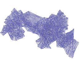
Among the most popular approaches are g2 o ("general        constraint is modeled with the information matrix Ωij and
graph optimization") [2]), Ceres Solver [9], GTSAM             the error function eij . This is illustrated in Figure 2b.
("Georgia Tech Smoothing and Mapping") [6], and SE-
Sync ("Synchronization over Special Euclidean group
SE(n)") [10]. There are few works in the literature that
compare some of these approaches. For example, in [11]
the authors provide an overview of visual SLAM and
compare g2 o, GTSAM, and HOG-Man [12] as back-ends.
The authors in [13] discuss the importance of rotation
estimation in pose graph estimation and compare g2 o and
GTSAM on benchmarking datasets with different rotation
estimation techniques. In [14], the authors compare dif-
ferent optimization algorithms under g2 o framework. A
unified SLAM framework, GLSLAM, proposed in [15],
provides various SLAM algorithm implementations, but                                             (a)
can also perform benchmarks for different SLAM ap-
proaches. However, to our knowledge, there are none
that compare g2 o, Ceres, GTSAM and SE-Sync in a
unified manner. The aim of this paper is to describe these
approaches in a unified manner and to evaluate them on an
array of publicly available synthetic and real-world pose
graph datasets (visualized in Figure 1). In the future, we
would like to use this comparison to facilitate the choice
of the PGO method.
   The paper is organized as follows. Section II describes
nonlinear graph optimization in general and each of these
four approaches. The experiment is the main part of this
paper and is described in Section III. In the first part of                                      (b)

the section, the hardware, the experimental setup, and the     Fig. 2: A pose-graph representation of the SLAM problem. (a) Every
benchmarking datasets are described. The results of the        node corresponds to a robot pose. Neighboring poses are connected
                                                               with edges. The edges model spatial constraints between two poses.
experiment are discussed at the end of the section. In the     The edges between contiguous poses represent odometry and remaining
end, Section IV concludes the paper.                           edges represent repeated observation of the same part of the environment
                                                               (loop closures). (b) Each edge is defined with its error function eij and
     II. N ONLINEAR P OSE - GRAPH O PTIMIZATION                information matrix Ωij . Error function is the difference between the
                      A PPROACHES                              real measurements zij and the approximated constraints ẑij (xi , xj ).

   Every pose graph consists of nodes and edges. The              Traditionally, the solution to (1) is obtained by it-
nodes in a pose graph correspond to the poses of the           erative optimization techniques (e.g., Gauss-Newton or
robot in the environment, and the edges represent spatial      Levenberg-Marquardt). Their idea is to approximate the
constraints between them. The edges between contiguous         error function with its first-order Taylor expansion around
nodes are odometric constraints, and the remaining edges       the current initial guess. In general, they consist of four
represent loop closing constraints. This is visualized in      main steps:
Figure 2a. The goal of pose graph optimization is to find
                                                                  1) Fix an initial guess.
a configuration of nodes that minimizes the least squares
                                                                  2) Approximate the problem as a convex problem.
error over all constraints in the pose graph. In general,
                                                                  3) Solve 2) and set it as a new initial guess.
a nonlinear least squares optimization problem can be
                                                                  4) Repeat 2) until convergence.
defined as follows:
                                                               Pose SLAM is easier to solve because it does not build
                   x∗ = argmin F(x),                     (1)   a map of the environment. Graph formulated problems
                             x
                                                               have sparse structure, so computation is faster. Another
where F(x) is the sum of errors over all constraints in        advantage is that it is robust to bad initial guesses. The
the graph:                                                     disadvantage of pose SLAM is that it is generally not
                      X                                        robust to outliers and does not converge when there are
              F(x) =        e>
                             ij Ωij eij .           (2)
                                                               many false loop closures. Moreover, rotation estimation
                         hi,ji∈C
                                                               makes it a hard noncovex optimization problem, so con-
Here, C represents the set of index pairs between con-         vex relaxation leads to problems with local minima and
nected nodes, Ωij represents the information matrix be-        there is no guarantee of a global optimum. In this section,
tween nodes i and j, and eij is the nonlinear error function   we briefly describe the optimization frameworks based on
that models how well the poses xi and xj satisfy the           the nonlinear least squares method that provide solutions
constraint imposed by the measurement zij . Finally, each      in the form of pose graphs.
A. g2 o pose-graph SLAM (in robotics), camera motion estima-
g2 o [2] is an open-source general framework for opti- tion (in computer vision), and sensor network localization
mization of nonlinear functions that can be defined as (in distributed sensing). Authors state in [10] that SE-
graphs. Its advantages are that it is easily extensible, Sync improves on previous methods by exploiting a novel
efficient, and applicable to a wide range of problems. The (convex) semidefinite relaxation of the special Euclidean
authors state in [2] that their system is comparable to other synchronization problem to directly search for globally
state-of-the-art algorithms while being highly general and optimal solutions, and is able to generate a computa-
extensible. They achieve efficiency by exploiting sparse tional certificate of correctness for the found solution.
connectivity and the special structure of the graph, using They apply truncated-Newton Riemannian Trust-Region
advanced methods to solve sparse linear systems, and uti- method [24] to find efficient estimates of poses.
lizing the features of modern processors. The framework III. E XPERIMENTS
contains three different methods that solve PGO, Gauss-
Our goal is to experimentally evaluate the optimization
Newton, Levenberg-Marquardt and Powell’s Dogleg. It
frameworks described in Section II and compare them.
is mainly used to solve the SLAM problem in robotics
For this purpose, we are considering their performance
and the bundle adjustment problems in computer vision.
in terms of total computation time and final value of
ORB-SLAM ( [16], [17]) uses g2 o as a back-end for
the objective function described by (2). We use publicly
camera pose optimization, and SVO [18] uses it for visual
available synthetic and real-world benchmarking datasets.
odometry.
B. Ceres A. Experimental setup
Ceres Solver [9] is an open-source C++ library for The experiment was conducted on a Lenovo ThinkPad
modeling and solving large, complicated optimization P50 equipped with an octa-core Intel Core i7-6700HQ
problems. It is mainly dedicated to solving nonlinear CPU operating at 2.60 GHz and 16 GB RAM. The
least squares problems (bundle adjustment and SLAM), computer is running Ubuntu 20.04. The same solver,
but can also solve general unconstrained optimization Levenberg-Marquardt, is chosen for the g2 o, Ceres and
problems. The framework is easy to use, portable, and GTSAM frameworks, while SE -Sync uses the Rieman-
extensively optimized to provide solution quality with low nian trust-region (RTR) method ( [24]). Each algorithm
computation time. Ceres is designed to allow the user to is limited to a maximum of 100 iterations. The stopping
define and modify the objective function and optimization criteria are based on reaching the maximum number of
solvers. The solvers that are implemented include trust iterations and the relative error decrease. SE-Sync uses a
region solvers (Levenberg-Marquardt, Powell’s Dogleg) slightly different method, so an additional criterion based
and line search solvers. Since it has many advantages, on the Riemann gradient norm must be specified. The
Ceres is used in many different applications and domains. tolerance for the relative error decrease is set to 10−5 and
OKVIS ( [19], [20]) and VINS [21] use Ceres to optimize the norm of the gradient is set to 10−2 . The parameters
nonlinear problems defined as graphs. are chosen according to the recommendations in [10].
The authors in [13] study the influence of orientation
C. GTSAM initialization on finding the global optimum. Inspired by
GTSAM [6] is another open-source C++ library that this work, we also do the pose graph initialization before
implements sensor fusion for robotics and computer vi- the optimization process. To achieve better results, we
sion applications. It can be used to solve optimization obtain initial pose graphs using the spanning tree method
problems in SLAM, visual odometry, and structure from [2].
motion (SfM). GTSAM uses factor graphs [22] to model
B. Benchmarking datasets
complex estimation problems and exploits their sparsity
to be computationally efficient. It implements Levenberg- There are six two-dimensional pose graphs obtained
Marquardt and Gauss-Newton style optimizers, the conju- from [25], two real-word graphs, and four graphs created
gate gradient optimizer, Dogleg, and iSAM: inceremen- in simulation. INTEL and MIT pose graphs are real-
tal smoothing and mapping. GTSAM is used alongside world datasets created by processing raw wheel odometry
various sensor front-ends in academia and industry. For and laser range sensor measurements collected at the Intel
instance, there is a variant of SVO [23] that uses GTSAM Research Lab in Seattle and MIT Killian Court. M3500
as a back-end for visual odometry. pose graph is a simulated Manhattan world [26]. The
M3500a, M3500b, and M3500c datasets are variants of
D. SE-Sync the M3500 dataset with Gaussian noise added to the
SE-Sync [10] is a certifiably correct algorithm for relative orientation measurements. The standard deviation
performing synchronization over the special Euclidean of the noise is 0.1, 0.2, and 0.3 rad, respectively. There
group. It’s objective is to estimate the values of a set of are also six three-dimensional datasets obtained from [13].
unknown poses (positions and orientations in Euclidean The pose graphs Sphere-a, Torus, and Cube are created
space) given noisy measurements of relative transforma- in simulation. Sphere-a dataset is a challenging prob-
tions between nodes. Their main applications are in the lem released in [27]. The other three pose graphs are
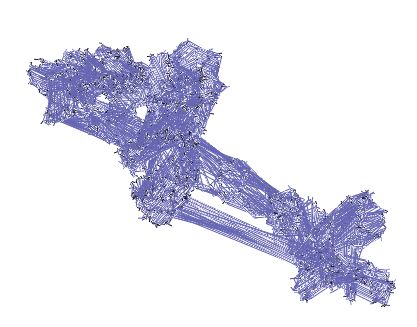
context of 2D and 3D geometric estimation. For example, real-world datasets. The Garage dataset was introduced(a) (b) (c) (d)
Fig. 3: Optimized pose graphs from (a) INTEL, (b) MIT, (c) M3500 and (d) M3500a datasets. Results are color coded for each algorithm: pink -
g2 o, green - Ceres, red - GTSAM, blue - SE-Sync.
g2 o Ceres GTSAM SE-Sync TABLE I: Pose-graph datasets with number of nodes and edges
Dataset Nodes Edges
Sphere-a 3D 2200 8647
Torus 3D 5000 9048
Cube 3D 8000 22236
Garage 3D 1661 6275
Cubicle 3D 5750 16869
(a)
Rim 3D 10195 29743
Intel 2D 1228 1483
MIT 2D 808 827
M3500 2D 3500 5453
M3500a 2D 3500 5453
M3500b 2D 3500 5453
(b) M3500c 2D 3500 5453
C. Results
We summarized all the performance results in Table
II in terms of total computation time and the value of
the objective function (2). For each dataset, we state
(c) the termination reason of the algorithm. The algorithm
converges if it completes the optimization within the
maximum iteration limit. We also give the validation time
for SE-Sync to certify the global optimum. Figures 3, 4
and 5 show optimized pose graphs for the benchmarking
problems.
(d) 1) INTEL: INTEL is one of the easiest problems to
solve. All approaches have solved it successfully. The
trajectories are shown together in Figure 3a and it can be
seen that all of them achieved a similar result. GTSAM
took the longest time to finish the optimization, but
achieved the lowest objective function value. SE-Sync is
(e) the fastest in this case and has the value slightly larger
Fig. 4: Results on five challenging datasets: (a) M3500b, (b) M3500c, (c)
than GTSAM. Considering this, SE -Sync seems to be
Sphere-a, (d) Cubicle, (e) Rim for each algorithm. From left to right: g2 o the best solution.
(pink), Ceres (green), GTSAM (red), SE-Sync (blue). SE-Sync shows 2) MIT: MIT is the smallest problem, but has only a
superior results, but GTSAM performs just as well on Cubicle and Rim
dataset.
few loop closure constraints. Therefore, it is important to
start the optimization with a good initial guess. Otherwise,
GTSAM, Ceres, and g2 o are not able to converge to a
in [28], and Cubicle and Rim are acquired using ICP on meaningful solution with the Levenberg-Marquardt algo-
point clouds from the 3D laser sensor at the RIM center rithm. All algorithms converged in less than the maximum
at Georgia Tech. All these pose graphs are visualized in number of iterations and they achieved almost the same
Fig. 1 with their odometric and loop-closing constraints. objective function values. The optimization problem is
Table I contains the number of nodes and edges for solved in less than half a second, but Ceres and g2 o are the
each dataset. These numbers determine the number of fastest. Ceres also achieved the lowest objective function
parameters in the optimization process and the complexity value and seems to be the best solver for the dataset MIT.
of the problem. The final trajectories can be seen in Figure 3b.TABLE II: Optimization times and objective values for each algorithm and dataset are organized in the table. Total time corresponds to elapsed
optimization time, and F(x) to the value of the objective function. Termination reason for each dataset is given: maximum number of iterations
reached (iter), relative function decrease (conv), divergence (no conv) and maximum level of Riemannian staircase (r max). Validation time for
SE-Sync is the time it takes for the algorithm to check the optimality of the solution. The minimum optimization time is marked in red, and the
lowest objective value is written in green. The blue color corresponds to the other minimum objective values with the poor visual representations
of the trajectory, or the same as the value marked in green.
INTEL MIT M3500 M3500a M3500b M3500c Sphere-a Torus Cube Garage Cubicle Rim
total time (s) 0.28 0.07 0.66 0.86 1.90 2.08 8.07 10.66 599.05 1.53 338.06 243.12
g2o F(x) 6.17E+04 4.12E+01 1.38E+02 9.12E+02 9.27E+03 6.61E+03 8.58E+05 1.46E+04 4.92E+04 1.24E+00 9.38E+07 1.45E+09
termination iter conv conv conv iter iter conv conv conv conv iter iter
total time (s) 0.04 0.06 0.23 0.31 1.56 0.76 18.87 2.04 62.59 0.73 25.66 49.82
Ceres F(x) 6.40E+05 1.89E+01 6.90E+01 4.56E+02 2.88E+03 1.86E+03 1.56E+06 1.21E+04 4.22E+04 6.34E-01 7.26E+06 1.01E+08
termination conv conv conv conv iter conv iter conv conv conv iter iter
total time (s) 21.55 0.16 0.41 1.23 3.88 1.30 12.16 2.34 113.89 0.66 2.54 19.41
GTSAM F(x) 1.14E+02 2.06E+01 6.90E+01 4.56E+02 3.60E+07 5.33E+06 3.30E+06 1.21E+04 4.22E+04 6.34E-01 1.36E+03 4.11E+04
termination iter conv conv conv no conv no conv conv conv conv conv conv conv
total time (s) 0.01 0.15 1.57 0.24 0.37 0.56 0.15 0.44 8.53 1.07 5.58 4.21
F(x) 1.97E+02 3.06E+01 9.69E+01 7.99E+02 1.84E+03 2.29E+03 1.48E+06 1.21E+04 4.22E+04 6.31E-01 3.59E+02 2.73E+03
SE-Sync
validation (s) 0.165 1.749 15.716 1.426 52.891 10.202 0.188 0.51 14.452 5.521 12.052 35.851
termination conv conv conv conv r max conv conv conv conv conv conv conv
(a) (b) (c)
Fig. 5: Final trajectories for (a) Torus, (b) Cube and (c) Garage dataset. Color codes are the same as in Figure 3.
3) M3500: All four variants of the M3500 dataset are g2 o and 100 times faster than Ceres and GTSAM. The
presented here together. GTSAM and Ceres are the best optimal solution by SE-Sync is shown in Figure 4c with
at solving the basic M3500 problem, as both achieve local optima obtained by the other three approaches.
the lowest objective function value, but Ceres is slightly 5) Torus: Torus is one of the easiest 3D problems. All
faster. All approaches were successful in solving the approaches except g2 o converge to the global optimum,
problem, and their optimized pose graphs are visualized but again SE-Sync wins in speed. g2 o solves the problem,
in Figure 3c. M3500a is a more difficult problem due to but looking at Figure 5a it can be seen that its optimized
the noise added to the relative orientations. Nevertheless, trajectory drifts slightly in comparison to the other three.
all approaches solved it, but as it can be seen in Figure 3d, 6) Cube: The cube dataset is more complex and time
the g2 o solution deviates from other solutions. Ceres consuming due to the large number of nodes and edges,
and GTSAM converged to the lowest value, but again but all approaches have found a solution. SE-Sync is by
Ceres is faster. M3500b and M3500c are very challenging far the fastest in solving this problem. It takes 8 seconds,
problems because the amount of noise is high. GTSAM while others take more than a minute. Final solutions are
does not converge in these two cases, and Ceres and shown in Figure 5b.
g2 o get stuck in a local minimum. SE-Sync is the most 7) Garage: The Garage dataset is the smallest and
successful approach in solving these two variants of the easiest 3D dataset to solve, for which each approach
problem. Considering the lack of loop closure constraints achieved a solution. This is illustrated in Fig. 5c. Ceres,
connecting the left and right parts of the pose graph, and GTSAM and SE-Sync converge to the same objective
the amount of noise in the measurements, SE-Sync has value, and GTSAM is the fastest in this case.
achieved a reasonably good solution. These pose graphs 8) Cubicle and Rim: The Cubicle dataset is a subset
can be seen in Figures 4a and 4b. of the Rim dataset, so we discuss them together. These
4) Sphere-a: The Sphere-a problem is also challenging two datasets are challenging because they both contain
because high amount of noise is added to the relative large number of nodes and edges. Moreover, large number
orientation measurements. Even with an initial guess, only of edges are false loop closures. Only GTSAM and SE-
SE-Sync was able to solve it. It converges to the global Sync converged to a solution in both cases. The pose
minimum in only 0.15 s which is 50 times faster thangraphs after optimization are visualized in Figures 4d [9] S. Agarwal, K. Mierle, and Others, “Ceres solver,” http://
and 4e. Ceres and g2 o are unable to find a solution. ceres-solver.org.
[10] D. Rosen, L. Carlone, A. Bandeira, and J. Leonard, “SE-Sync: A
GTSAM solves the Cubicle two times faster than SE- certifiably correct algorithm for synchronization over the special
Sync, but SE-Sync converges to the global optimum. SE- Euclidean group,” Intl. J. of Robotics Research, vol. 38, no. 2–3,
pp. 95–125, Mar. 2019.
Sync optimizes the Rim five times faster than GTSAM [11] D. M. a. Latif, M. a. Megeed Salem, H. Ramadan, and M. I.
and converges to the global optimum. Roushdy, “Comparison of Optimization Techniques for 3D Graph-
based,” Proceedings of the 4th European Conference of Computer
IV. C ONCLUSION Science (ECCS ’13) Recent Advances in Information Science, p.
In this paper, we compared graph optimization meth- 288, 2013.
[12] G. Grisetti, R. Kümmerle, C. Stachniss, U. Frese, and
ods used for pose estimation in SLAM. We considered C. Hertzberg, “Hierarchical optimization on manifolds for online
g2 o and GTSAM, which are current state-of-the-art ap- 2d and 3d mapping,” in 2010 IEEE International Conference on
proaches, Ceres, a user-friendly open-source framework, Robotics and Automation, 2010, pp. 273–278.
[13] L. Carlone, R. Tron, K. Daniilidis, and F. Dellaert, “Initialization
and SE-Sync, a novel and robust method for pose synchro- techniques for 3D SLAM: A survey on rotation estimation and its
nization. The evaluation process takes into account the use in pose graph optimization,” in Proceedings - IEEE Interna-
elapsed optimization time and the value of the objective tional Conference on Robotics and Automation, vol. 2015-June,
no. June. Institute of Electrical and Electronics Engineers Inc.,
function, and the results are given in the form of a table jun 2015, pp. 4597–4604.
for twelve benchmarking datasets. [14] H. Li, Q. Zhang, and D. Zhao, “Comparison of methods to
SE-Sync achieved the smallest total time on most efficient graph SLAM under general optimization framework,”
in Proceedings - 2017 32nd Youth Academic Annual Conference
datasets when compared to other three methods. It is of Chinese Association of Automation, YAC 2017. Institute of
also able to validate the certificate of global optimality if Electrical and Electronics Engineers Inc., jun 2017, pp. 321–326.
required, but at the cost of additional computation time. [15] Y. Zhao, S. Xu, S. Bu, H. Jiang, and P. Han, “Gslam: A general
slam framework and benchmark,” in 2019 IEEE/CVF International
g2 o had the highest total time but performed well on Conference on Computer Vision (ICCV), 2019, pp. 1110–1120.
simple 2D datasets. Ceres is easy to use, offers a lot of [16] R. Mur-Artal, J. M. Montiel, and J. D. Tardos, “ORB-SLAM: A
flexibility, and is relatively fast. GTSAM performs almost Versatile and Accurate Monocular SLAM System,” IEEE Trans-
actions on Robotics, vol. 31, no. 5, pp. 1147–1163, oct 2015.
as well as SE-Sync, except on very noisy 2D datasets. [17] R. Mur-Artal and J. D. Tardos, “ORB-SLAM2: An Open-Source
Paired with a proper front-end, these methods can be SLAM System for Monocular, Stereo, and RGB-D Cameras,”
very powerful in solving SLAM problems. For poor data IEEE Transactions on Robotics, vol. 33, no. 5, pp. 1255–1262,
oct 2017.
association, high noise, and a poor performing front-end, [18] C. Forster, M. Pizzoli, and D. Scaramuzza, “SVO: Fast semi-direct
it seems best to use SE-Sync as the back-end. With a good monocular visual odometry,” in Proceedings - IEEE International
initialization method, GTSAM seems to do an equally Conference on Robotics and Automation. Institute of Electrical
and Electronics Engineers Inc., sep 2014, pp. 15–22.
good job. If the front-end is excellent, dataset relatively [19] S. Leutenegger, S. Lynen, M. Bosse, R. Siegwart, and P. Furgale,
simple, or the noise is low, it is a matter of personal “Keyframe-based visual-inertial odometry using nonlinear opti-
preference to decide between these back-ends. We hope mization,” International Journal of Robotics Research, vol. 34,
no. 3, pp. 314–334, 2015.
this comparison can help other researchers in choosing a [20] S. Leutenegger, P. Furgale, V. Rabaud, M. Chli, K. Konolige,
back-end method for their SLAM applications. and R. Siegwart, “Keyframe-Based Visual-Inertial SLAM using
Nonlinear Optimization,” Tech. Rep., 2016.
R EFERENCES [21] T. Qin, P. Li, and S. Shen, “VINS-Mono: A Robust and Versatile
[1] F. Lu and E. Milios, “Globally Consistent Range Scan Alignment Monocular Visual-Inertial State Estimator,” Tech. Rep. 4, 2018.
for Environment Mapping,” Autonomous Robots, vol. 4, no. 4, pp. [22] F. Dellaert and M. Kaess, “Factor Graphs for Robot Perception,”
333–349, 1997. Foundations and Trends in Robotics, vol. 6, no. 1-2, pp. 1–139,
[2] R. Kümmerle, G. Grisetti, H. Strasdat, K. Konolige, and W. Bur- 2017.
gard, “G2o: A general framework for graph optimization,” in [23] C. Forster, L. Carlone, F. Dellaert, and D. Scaramuzza, “On-
Proceedings - IEEE International Conference on Robotics and Manifold Preintegration for Real-Time Visual-Inertial Odometry,”
Automation, 2011, pp. 3607–3613. IEEE Transactions on Robotics, vol. 33, no. 1, pp. 1–21, feb 2017.
[3] F. Dellaert and M. Kaess, “Square root SAM: Simultaneous [24] P.-A. Absil, C. Baker, and K. Gallivan, “Trust-region methods on
localization and mapping via square root information smoothing,” Riemannian manifolds,” Found. Comput. Math., vol. 7, no. 3, pp.
International Journal of Robotics Research, vol. 25, no. 12, pp. 303–330, Jul. 2007.
1181–1203, 2006. [25] L. Carlone and A. Censi, “From angular manifolds to the integer
[4] M. Kaess, A. Ranganathan, and F. Dellaert, “iSAM: Incremental lattice: Guaranteed orientation estimation with application to pose
smoothing and mapping,” IEEE Transactions on Robotics, vol. 24, graph optimization,” IEEE Transactions on Robotics, vol. 30, no. 2,
no. 6, pp. 1365–1378, 2008. pp. 475–492, 2014.
[5] M. Kaess, H. Johannsson, R. Roberts, V. Ila, J. J. Leonard, [26] E. Olson, J. Leonard, and S. Teller, “Fast iterative alignment of
and F. Dellaert, “ISAM2: Incremental smoothing and mapping pose graphs with poor initial estimates,” in Proceedings - IEEE
using the Bayes tree,” International Journal of Robotics Research, International Conference on Robotics and Automation, vol. 2006,
vol. 31, no. 2, pp. 216–235, 2012. 2006, pp. 2262–2269.
[6] F. Dellaert, V. Agrawal, A. Jain, M. Sklar, and M. Xie, “GTSAM,” [27] C. Stachniss, U. Frese, and G. Grisetti, “Openslam,” http://www.
https://gtsam.org. openslam.org/.
[7] R. M. Eustice, H. Singh, and J. J. Leonard, “Exactly Sparse [28] R. Kümmerle, D. Hähnel, D. Dolgov, S. Thrun, and W. Bur-
Delayed-State Filters for View-Based SLAM,” IEEE Transactions gard, “Autonomous driving in a multi-level parking structure,”
on Robotics, vol. 22, no. 6, pp. 1100–1114, 2006. in Proceedings - IEEE International Conference on Robotics and
[8] K. Lenac, J. Ćesić, I. Marković, and I. Petrović, “Exactly sparse Automation, 2009, pp. 3395–3400.
delayed state filter on Lie groups for long-term pose graph SLAM,”
International Journal of Robotics Research, vol. 37, no. 6, pp.
585–610, 2018.You can also read