A detailed model of gene promoter dynamics reveals the entry into productive elongation to be a highly punctual process.
←
→
Page content transcription
If your browser does not render page correctly, please read the page content below
A detailed model of gene promoter dynamics reveals the entry
                                                 into productive elongation to be a highly punctual process.

                                                                                      Jaroslav Albert
                                                                            jaroslav.albert@ronininstitute.org
                                                                                       Ronin Institute
arXiv:2201.13092v1 [q-bio.MN] 31 Jan 2022

                                                                                          Abstract
                                              Gene transcription is a multistep stochastic process that involves thousands of reactions. The
                                            first set of these reactions, which happen near a gene promoter, are considered to be the most
                                            important in the context of stochastic noise and have been a focus of much research. The most
                                            common models of transcription are primarily concerned with the effect of activators/repressors
                                            on the overall transcription rate and approximate the basal transcription processes as a one step
                                            event. According to such effective models, the Fano factor of mRNA copy distributions is always
                                            greater than (super-Poissonian) or equal to 1 (Poissonian), and the only way to go below this
                                            limit (sub-Poissonian) is via a negative feedback. It is partly due to this limit that the first
                                            stage of transcription is held responsible for most of the stochastic noise in mRNA copy numbers.
                                            However, by considering all major reactions that build and drive the basal transcription machinery,
                                            from the first protein that binds a promoter to the entrance of the transcription complex (TC) into
                                            productive elongation, it is shown that the first two stages of transcription, namely the pre-initiation
                                            complex (PIC) formation and the promoter proximal pausing (PPP), is a highly punctual process.
                                            In other words, the time between the first and the last step of this process is narrowly distributed,
                                            which gives rise to sub-Poissonian distributions for the number of TCs that have entered productive
                                            elongation. In fact, having simulated the PIC formation and the PPP via the Gillespie algorithm
                                            using 2000 distinct parameter sets and 4 different reaction network topologies, it is shown that
                                            only 4.4% give rise to a Fano factor that is > 1 with the upper bound of 1.7, while for 31% of
                                            cases the Fano factor is below 0.5, with 0.19 as the lower bound. The two parameters that exert
                                            the most control on the Fano factor are the binding and dissociation rates between the activator
                                            and its enhancer. In the limit as these rates become low, our model approaches the conventional
                                            two-state promoter model, which can give rise Fano factors much larger than one. These results
                                            cast doubt on the notion that most of the stochastic noise observed in mRNA distributions always
                                            originates at the promoter.

                                                                                              1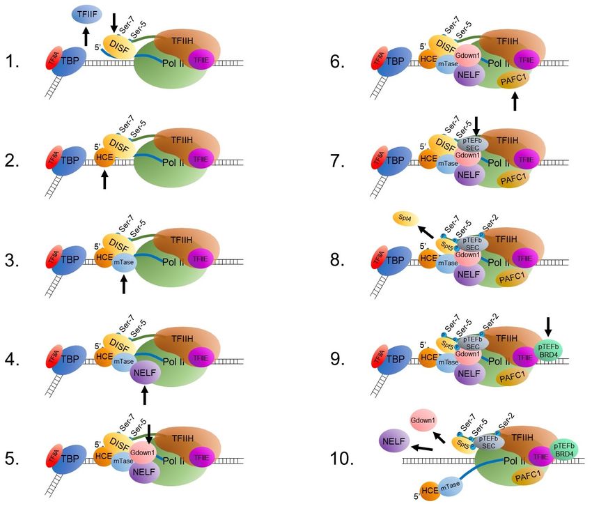
INTRODUCTION

   Gene transcription is a stochastic process involving a multitude of biochemical reactions
by which the genetic code of a gene is copied into messenger RNA (mRNA). In eukaryotes,
transcription occurs in four stages: 1) pre-initiation complex (PIC) formation [1–3]; 2) pro-
moter proximal pausing (PPP) [4–10]; 3) productive elongation [11–13]; and 4) termination
[14–21]. In stage 1) general transcription factors (GTF) bind the promoter in order to re-
cruit RNA Polymerase II (Pol II) and other GTFs that enable the Pol II complex to begin
transcription. In stage 2) the Pol II complex pauses a short distance downstream from the
promoter site in order to give time to necessary processes, such as RNA capping and the
addition of elongation-promoting factors, to do their job. In stage 3) the Pol II complex -
known at this stage as elongation complex (EC) - enters the main body of a gene where it
continues to transcribe mRNA until stage 4) in which transcription is terminated and the
completed mRNA, along with the Pol II complex, are released. There are additional stages,
such as splicing and the synthesis of ribonucleoprotein particles [22]; however, these tend
to occur (though not always) during the elongation stage and can be incorporated into the
elongation process itself [23].

   Traditionally, stochastic models of transcription tend to focus on a highly simplified
version of stage 1), while either ignoring the subsequent stages [24] or handling them by in-
troducing a delay [25]. By doing so, such models are forced to operate under the assumption
that whatever noise in mRNA copy numbers they are meant to explain/simulate, it all comes
from this first stage. For super-Poissonian distributions, these models do quite well, owing
to the multitude of promoter states that can be produced via activators/repressors. On the
other hand, for sub-Poissonian distributions, this class of models works only in the presence
of a negative feedback and only under certain conditions [26–29]. However, models that take
into account the reinitiation of Pol II at the promoter have revealed that mRNA distribu-
tions can in fact be sub-Poissonian without any feedback [30], or at the very least reduce
the variance [31–38] as compared to the above-mentioned simpler models. This discovery
challenges the conventional wisdom that sub-Poissonian mRNA distributions are necessarily
indicative of a negative feedback.

   In this paper, we present a detailed stochastic model of the PIC formation and the PPP,
one that involves 15 macromolecules - 13 general transcription factors (GTF), 1 activator,

                                            2
and the RNA polymerase II. The model is based on the current understanding of these two
transcription stages. The goal of this paper is to investigate the range of Fano factors for
the number distribution of ECs in a given time. we do this by generating 500 parameter
sets and simulate for each set the stochastic evolution of the system, starting with an empty
promoter. A crucial feature of this model is the relationship between the PPP stage and
the reinitiation of Pol II, which can take several forms, two of which are considered herein:
1) Pol II is able to bind the promoter only when the promoter proximal region is free of a
paused complex (PC); and 2) Pol II can bind but it cannot clear the promoter while a PC is
present. The effects of activator dynamics on the resulting Fano factors are also simulated
using a simple on-off model, where “on” means the activator is bound to the promoter and
“off” means it is not. Since the exact order in which the GTFs are recruited to the promoter
is still unsettled, all simulations are repeated using models with one and two additional
reaction pathways. The simulations show a remarkable reluctance of the Fano factors to rise
above 1 when the activator dynamics are relatively fast. In those cases where the binding
rate is fast and the dissociation rate is slow, the Fano factors concentrate around the value
of 0.4 with a maximum of 0.6. On the other hand, when both the binding and dissociation
factors are low, the Fano factors can reach values in excess of xxx. While the correlation
between the activator dynamics and the Fano factors is consistent with previous studies, the
migration of the Fano factors to such extremely low values is a novel feature of the highly
sequential nature of stages 1) and 2).

  GENE TRANSCRIPTION

  Pre-initiation complex formation

  The first step in mRNA transcription is the pre-initiation complex (PIC), the formation of
which begins with the binding of a transcription factor (TF) called TFIID to the promoter.
TFIID is a multi sub-unit factor comprising of TBP (TATA binding protein) and TAFs
(TBP associated factors). As the name suggests, the TBP binds to the part of the promoter
with the sequence TATA (Fig. 1.1 and 1.2). When the TBP binds the TATA box, it creates
an almost 80 degree bend in the DNA. In order to stabilize this TATA-TBP complex, another
TF, called TFIIA, binds to it (Fig. 1.3). Strictly speaking, TFIIA is not a general TF, as

                                            3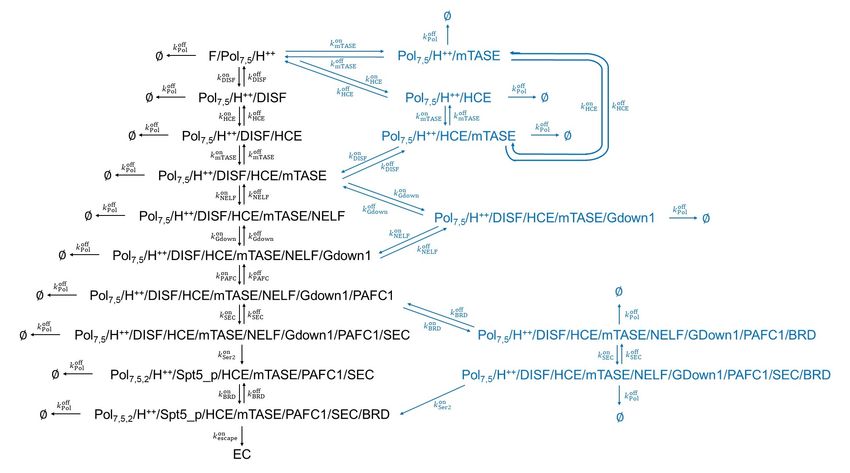
FIG. 1. Pre-clearance complex (PCC) formation. 1) Empty promoter; 2) TBP binds to
TATA box and bends the DNA; 3) TFIIA binds TBP; 4) TFIIB binds the TATA/TBP complex;
5) the complex Pol II/TFIIF is recruited; 6) the complex TFIIH/TFIIE is recruited; 7) initiation:
DNA unwinds; 8) Serine 7 is phosphorelated, bubble grows and TFIIB is released; 9) Serine 5 is
phosphorelated; 10) the EC clears the promoter.

transcription can proceed without it, but merely functions as a scaffold protein. The TF that
is crucial for transcription is TFIIB (Fig. 1.4), which can bind the promoter independently
of TFIIA. In this state, the promoter can receive the RNA polymerase II (Pol II). Since Pol
II has no affinity to the DNA, it must bind the promoter via a TF called TFIIF (Fig. 1.5),
which has affinity to TFIIB. The TFIIB has a part that binds the promoter, and another
part, called the B-reader, that ensured that Pol II faces the downstream direction. Another
role of TFIIF is to recruit TFIIE, which acts as a loading factor for another TF called TFIIH.
TFIIE and TFIIH usually bind the promoter as a complex (Fig. 1.6). In higher eukaryotes
– which is the focus of this paper – all these processes are happening in a 3-dimensional

                                              4
confirmation with the help of long range enhancers and mediator proteins, which together
form the enhancer-mediator complex. For simplicity, the mediator or the enhancers were
are not shown in Fig. 1.

   Initiation

   At this point the DNA is still closed and the Pol II is not yet making any mRNA.
However, soon after TFIIH comes into play, the DNA unwinds in the activity center of Pol
II (Fig. 1.7). What causes this unwinding is a tug of war between TFIIH and TBP. Pol II
is a processive enzyme and wants to move forward. However, because it is bound to TFIIB
via TFIIF, it is unable to move. The XPB-subunit of TFIIH, which is the translocate part
of TFIIH, tracks the DNA forward, but because it is bound to Pol II via TFIIE, it, too,
cannot move. As a result of these opposing forces, the DNA unwinds. Such unwound DNA
is called a bubble [39]. At this stage the Pol II tries to synthesize mRNA but is blocked
by the B-reader part of TFIIB, which partially extends to the active site of Pol II. The
partial blocking of the B-reader ensures that Pol II begins transcription at the correct site,
called +1. Since this blocking is only partial, Pol II sometimes manages to produce short
transcripts ∼ 3-5 base pair long, which, unless the Pol II can clear the promoter, are released
from the active site – a process known as abortive transcription (not shown in the figure).
This transition from closed to open bubble is called initiation.

   Promoter clearance

   When the nascent RNA grows to a length of about 9 nucleotides, thus strengthening
the RNA-DNA bond, it becomes harder to abort. The growing transcript forces TFIIB
to dissociate, allowing the bubble to grow to a length of about 18 nucleotides (Fig. 1.8).
However, such a large bubble is thermodynamically unstable and collapses to a smaller
bubble of length of about 10 nucleotides. This collapse creates a force that causes a forward
movement of Pol II. At the time of the bubble collapse, the C-terminal domain (CTD) of
Pol II is phosphorylated (Fig. 1.8 and 1.9). This phosphorylation is facilitated by the CDK7
subunit of TFIIH and the enhancer-bound kineses, which add phosphate groups to Serine
7 and Serine 5 (in that order) of each heptad repeat of the CDT. Serine 5 phosphorylation

                                             5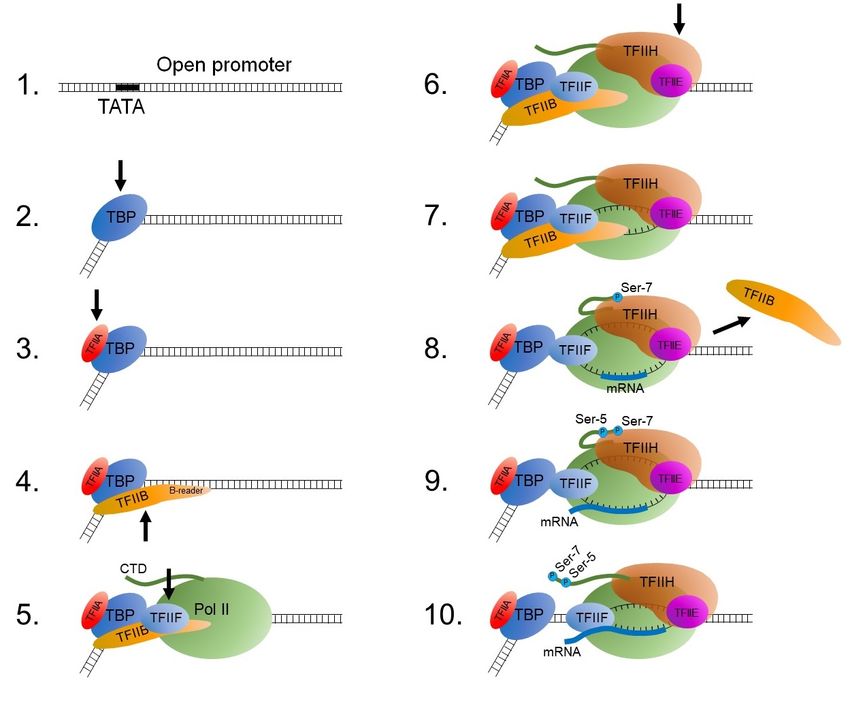
FIG. 2. Promoter proximal pausing and escape. 1) DISF is recruited by phosphorelated
Serine-5 and Serine-7 to the nascent mRNA; 2) HCE caps the 5’ end of mRNA; 3) mTASE is
recruited to the 5’ end; 4) NELF is recruited; 5) Gdown1 is recruited; 6) PAFC1 is recruited; 7)
the pTEFb/SEC complex is recruited; 8) the pTEFb/SEC complex phosphorelates Serine 2; 9)
the complex pTEFb/BRD is recrired; 10) escape into productive elongation.

breaks the bond between Pol II and the mediator complex, allowing Pol II to move forward
and increasing the transcript to a length of 20 base pairs on average (Fig. 1.10).

   Note: by conventional definition, PIC refers to the protein complex consisting of TBP,
TFIIA (optional), TFIIB, TFIIE, TFIIF, Pol II and TFIIH. For convenience we will define
the term “Pre-clearance complex” (PCC) to mean the state of the Pol II complex prior to
clearance in order to place the initiation and phosphorylation processes under one umbrella.

                                              6
Promoter proximal pausing and escape

  The 5’ end of the transcript is now sticking out of the Pol II exit channel. At this
time, Spt 4 and Spt 5, which togeher are known as the DSIF complex, are recruited to
the phosphorelated Serine-5 and Serine-7 of the CDK, while in the process removing TFIIF
(Fig. 2.1). The function of the DSIF complex is to recruit two capping enzymes, the human
capping enzyme (HCE) and mTASE, to the 5’ end of the transcript (Fig. 2.2 and 2.3),
which increases the stability of the RNA, and also to recruit a TF called NELF (negative
elongation factor) (Fig. 2.4). NELF freezes Pol II, thus locking the RNA-DNA hybrid inside
its active center. Another TF, called Gdown1, binds the growing complex (Fig. 2.5) and
helps NELF to maintain this frozen state. Gdown1 also prevents TFIIF from binding back
to Poll II and keeps protein called TTF2 (transcription termination factor 2) from binding
the complex. Another TF called PAFC1 (Pol associated factor complex 1) binds Pol II (Fig.
2.6); it has a dual role of promoting the frozen state and helps maintain elongation. To
overcome this frozen state, two special proteins BRD-4 and SEC bind a TF called pTEF-b,
thus stimulating its kinase activity. The pTEF-b/SEC complex changes the comformation
of PAFC1 and phosphorelates the Spt5 part of DISF and Seren-2 of the CTD, which releases
the Stp4 part of DISF in the process (Fig. 2.8). Now the PAFC1 and Spt5, which were
previously negative regulators in the promoter proximal state, are now positive regulators of
elongation and stay bound to Pol II. To complete the transition from the PPP to productive
elongation, pTEF-b/BRD-4 must bind the complex (Fig. 2.9), which stimulates the release
of Spt4, NELF and Gdown1, allowing Pol II to enter the elongation phase (Fig. 2.10).

  Reinitiation of Pol II

  When the Pol II complex clears the promoter, the promoter returns to one of the states
TATA, TATA/TBP or TATA/TBP/A. That means that the PIC can begin to form again.
However, due to structural reasons, e. g. the size of the PC (paused complex) and its
location on the gene, a newly bound Pol II may not have enough physical space to clear the
promoter [40–43]. The question as to whether another Pol II can even bind the promoter
in the presence of a PC or whether it is simply blocked from clearing has not been settled.
However, there is increasing evidence for a negative correlation between the amount of time

                                            7
FIG. 3. Reactions involved in the pre-clearance complex (PCC) formation.

the PC stays in the paused state and the clearance rate [44, 45].

  MATERIALS AND METHODS

  The model

  The biochemical reactions that form the PCC and those that cause and maintain the PC
are shown in Fig. 3 and 4, respectively. The variables, i. e. promoter states, are labeled
so as to make clear what proteins are bound to the complex and what parts of the complex
have been phosphorylated. For example, in the transition from TATA/TBP/B/F/Pol/H
to TATA/TBP/F/Pol+ /H, the complex has moved into the initiation phase, conveyed by
the plus sign, and TFII B was released in the process, as indicated by the absence of B
in the latter state. This transition changes the value of the former variable from 1 to 0,
and conversely so for the latter variable. The subscript in, e. g. TATA/TBP/F/Pol+
                                                                                 7,5 /H,

                                            8
FIG. 4. Reactions involved in the promoter proximal pausing and escape.
indicates that both Serine 7 and Serine 5 have been phosphorylated. In Fig. 4, the double
plus in the superscript of H signifies that the PCC has cleared the promoter. The reactions
that lead to the state ∅ cause Pol II to dissociate from the DNA. Hence, ∅, which also takes
on the values of 0 or 1, represents an empty DNA in the region downstream from the PCC.
Two distinct interactions between the PCC and PC were considered: 1) Pol II cannot bind
the promoter unless ∅ = 1; and 2) Pol II can bind the promoter but cannot clear it unless
on
∅ = 1. Thus, the reaction propensity for case 1) was kPol ∅, while the propensity in case 2)
was kclear ∅.
In addition to the reactions in Figs. 3 and 4, the following reactions were added to the
system:
on
kact
∅ −−− −→ Z
off
kact
Z −−− −→ ∅,
(1)
9where Z is the state of an enhancer, such that when Z = 1, the enhancer is occupied by an
activator, and when Z = 0, the enhancer is unoccupied. Although the mechanism by which
activators enhance transcription is not unique and can occur in both the PCC formation [46]
and during the PPP [47, 48], some evidence suggests that in the PCC formation the primary
role of activators is to bring Pol II to the promoter [49]. To keep things simple, we have
incorporated the state of the enhancer, i. e. the variable Z, into the main model by multiply-
ing the propensities for transitioning from the state TATA/TBP/B and TATA/TBP/A/B
to TATA/TBP/B/Pol and TATA/TBP/A/B/Pol, respectively, by (1 + 99Z)/100. The logic
on
behind this factor is simple. When Z = 0, and remains so (no activator, i. e. kact = 0),
on
the propensity for the binding of Pol II is kPol /100, which diminishes the overall rate of
transcription; we consider this as the state of basal transcription. When Z = 1, and remains
off on
so, i. e. kact = 0, the propensity for the binding of Pol II is restored to kPol . Finally, there
on off on off
is the intermediate situation, in which kPol 6= 0 and kPol 6= 0. By regulating kPol and kPol ,
one can not only adjust the overall transcription rate, but also the stochastic nose in the
system, as will be demonstrated later.
Parameter selection
The parameters used in all simulations were selected from ranges that are consistent with
values found in literature. Table 1 shows the parameter ranges for the PIC formation and
the relevant references.
For the PPP, specific reaction rates are much less available than the rates for the PIC
formation. However, since the reactions that occur during the PPP are of the same kind
as those in the PIC formation, namely association and dissociation of proteins, it is rea-
sonable to assume they too have ranges similar to those given in Table 1, e. g. 0.001-
0.1s−1 . Also, these rates can be constrained by the average duration of the pausing, for
which there are data. In, for example, [57], the average duration of the PPP, htpause i, was
measured to be ∼ 5 minutes. Note: in [57] and other studies, htpause i is not considered
to be the time it takes the freshly cleared complex to reach the elongation stage; rather
it is treated as the time that Pol II spends bound to the DNA during the paused state.
In other words, htpause i is the average waiting time for either ∅ to go from 0 to 1, or for
Pol++
7,5,2 /H/Spt5p /HCE/mTASE/PAFC1/SEC/BRD to transition into PE. Another limiting
10TABLE I. at nM = 8
Description Symbol Range Reference
Binding rate of TBP kTBP 0.001-0.1 s−1 [4, 50–52]
Binding rate of TFIIA kA 0.01-0.1 s−1 [50]
Binding rate of TFIIB kB 0.025-0.25 s−1 [50]
Binding rate of Pol II kPol 0.025-0.25 s−1 [53]
Dissociation rate of TBP kTBP 0.125-0.0125 s−1 [50, 52, 54–56]
Dissociation rate of TFIIA kA 0.01-0.001 s−1 [50, 52]
Dissociation rate of TFIIB kB 0.6-0.006 s−1 [50, 52, 54]
Average pause time tpause ∼5 mins [31, 57]
Efficiency r 5.5-83.3×10⁻⁴ s−1
factor that can help restrict not only the reaction rates of the PPP but the rates of the
PCC formation as well, is the efficiency of transcription, or transcription rate r, which is
typically in the range 5.5-83.3×10⁻⁴ s−1 . The rate r is defined as the inverse of the average
waiting time to reach productive elongation htelong i, starting from randomized initial condi-
tions, i. e. a value of one is randomly assigned to one of the variables TATA, TATA/TBP,
TATA/TBP/A, TATA/TBP/B, TATA/TBP/A/B at time t = 0. For the purposes of this
paper it is not necessary to compute htelong i exactly; an estimate is sufficient and can be
obtained by computing htclear i, which is the average waiting time for clearance to occur, sub-
ject to the aforementioned randomized initial conditions, and then adding htescape i, which is
defined as the time to go from the state F/Pol7,5 /H to PE (see Fig. 4). Thus, r = htelong i−1 ,
where htelong i ∼ htclear i + htescape i. The exact details on how htclear i, htescape i and htpause i were
computed can be found in appendix A.
We generated 500 parameter sets in the range restriction 0.001 − 0.1 and subject to the
constraints 4 < htpause i < 6 min and 13 × 10−4 s−1 < r < 20 × 10−4 s−1 . Evidence suggests
[50] that when TFIIA is bound to the promoter, the binding rate of TFIIB is significantly
enhanced, while its dissociation rate is much reduced. This was taken into account by
on
setting kA|B to 10kBon and kA|B
on
to 0.1kBon (see Fig. 3). Note that while binding factors
must have an upper bound, due to physical restrictions such as protein density, number
of collisions with their target, et cetera, no such restrictions apply to the lower bounds of
11dissociation factors; they are instead restricted by thermodynamic stability and degradation
by enzymatic reactions. Thus, the values of some dissociation factors below 10−3 s−1 were
allowed. They were also necessary, as we will now explain.
The aforementioned scheme for computing htpause i and estimating r was unable to gen-
erate r in the desired range 13 × 10−4 s−1 − 20 × 10−4 s−1 when all parameter values were
constrained to 0.001s−1 - 0.1s−1 ; the largest value of r yielded by this range after ten thou-
sand selections was 0.7 × 10⁻⁴ s−1 . For this reason, we decided to lower the dissociation
rate for Pol II in PCC (but not in the PC) by some factor β. Then, β was incrementally
increased until the scheme started producing the desired results. The lowest value of β that
yielded the desired results within ten thousand selections was 10. Thus, the range for the
dissociation rate for Pol II in PCC was set to 0.0001 − 0.01s−1 .
Simulations
All simulations were done with the Gillespie algorithm (GA) [58]. For all simulations, each
realization in an ensemble started at time t = 0, and with the initial conditions TATA= 1,
and stopped when the algorithm passed t = 60000s. The number of times the reaction
Pol++
7,5,2 /H/Spt5p /HCE/mTASE/PAFC1/SEC/BRD→ EC occurred before t = 60000s was
recorded. From now on, we will let EC represent this number. Note: the transcription rate
r is related to the average EC via r = hECi/60000. In all subsequent sections we will refer
to hECi, rather than r.
RESULTS
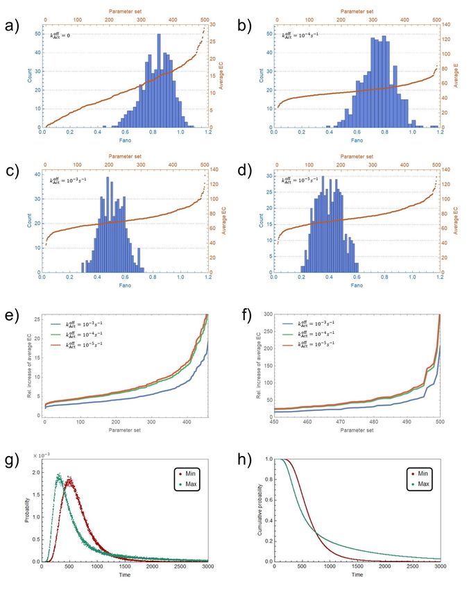
For each of the 500 parameter sets, using the PCC-PC interaction model 1) (see pre-
on off
vious section) a simulation was done with the following combinations of (kact , kact ): (0, 0),
(10−3 , 10−3 ), (10−3 , 10−4 ) and (10−3 , 10−5 ) (in inverse seconds). The averages and Fano
factors for the variable EC are presented in Fig. 5 a-d. The averages, represented by
the orange dots, are sorted in an ascending order. The histograms were constructed in
Mathematica using the “Histogram” function with 30 bars. Fig. 5 e and f show the in-
on off
crease in average EC upon introducing an activator for different combinations (kact , kact ),
represented by different colors. For each color, the curves were sorted in their own ascend-
12FIG. 5. Results of simulations for PCC-PC interaction model 1. (a) - (d): Fano factors (blue
bars) and average EC for all 500 parameter sets. (e) and (f ): Increase in average EC relative to
basal average EC in ascending order. (g): Probability distribution for times of entrance into PE
for the maximum (green) and minimum (red) Fano factor. (h): Cumulative distributions for the
curves in (g).
13FIG. 6. Comparison of results between PCC-PC interaction models 1 and 2. (a) - (d): Fano
distributions for PCC-PC interaction models 1 (orange) and model 2 (blue). (a) - (d): Increase in
average EC of PCC-PC interaction model 1 relative to PCC-PC interaction model 2 in ascending
order.
14on = k off = 0, k on = k off =
FIG. 7. Fano distributions (a) and averages of EC (b) for kAct Act Act Act
5 × 10⁻⁵ s−1 and kAct
on = k off = 10−5 s−1 .
Act
ing order. Shown in Fig. 5 g are two probability density functions P (t) for the reaction
Pol++
7,5,2 /H/Spt5p /HCE/mTASE/PAFC1/SEC/BRD→ EC to occur between the times t and
t + dt. Fig. 5 h shows the cumulative distribution functions Pc (t) defined as
Z t
Pc (t) = 1 − dt0 P (t0 ). (2)
0
The cumulative function, Eq. (2), is used to sample t by solving the equation Pc (t) = ξ,
where ξ is a random real number ranging from 0 to 1. The red (green) curve in both graphs
was generated from a parameter set responsible for the smallest (largest) Fano factor in all
the obtained data. Fig. 5 g reveals an interesting feature of this system: even though the
bulk of the red curve seems to be wider than that of the green curve, the green curve has
a much longer tail. If one was to sample the time at which a new EC occurred using the
cumulative functions in Fig. 5 h, the times that are greater than ∼800 seconds would occur
much more often for the green curve than the red curve.
This entire procedure was repeated for the second PCC-PC interaction (see previous
on off
section), the results of which are shown in Fig. 6. For all combinations of (kact , kact )
mentioned above, the Fano distributions tend slightly towards the right (see Fig. 6 a-d).
With this increased noise, the efficiencies also increase. It is clear from these graphs that
the distributions of EC tend to be sub-Poissonian regardless of the reaction rates. This is
off
more true the smaller kact on
is compared to kact = 10−3 s−1 .
on
However, what would happen if both kact off
and kact were small, e. g. ∼ 10−5 ? To answer
on
this question, I ran additional simulations for these combinations of (kact off
, kact ): (10−4 , 10−4 ),
(5 × 10⁻⁵ , 5 × 10⁻⁵ ) and (10−5 , 10−5 ) (in inverse seconds). The results shown in Fig. 7 a) are
consistent with previous research: the slower the activator dynamics, the greater the noise
15FIG. 8. Two additional pathways to get from F/Pol/7,5 /H++ to EC.
tends to be. The averages, shown in Fig. 7 b), do not seem to change very much compared
to those in Figs. 5 and 6.
Alternative pathways
The mechanism of the PCC formation and the PPP is still a subject of ongoing research
with many details to be worked out, as well as some major discoveries to be made. For
example, the precise order in which the two complexes are formed and whether they are
always formed the same way has not yet reached a consensus. Given such a state of affairs,
it is reasonable to wonder if the results obtained thus far would hold up if some of the
reactions in Figs. 3 and 4 could also happen in a different order. In other words, what
would happen if there were alternative pathways to get from an empty promoter to PE?
To answer this question, we ran simulations for the PCC-PC interaction model 1) but with
additional pathways, shown in Figs. 8 and 9. The reactions in blue are the additional
pathways. In Fig. 8, there are two additional pathways: HCE and mTASE bind before
DISF; and Gdown1 binds before NELF. In Fig. 9, there are two additional pathways on top
of those from Fig. 8: mTASE binds before HCE, followed by DISF; and BRD binds before
16FIG. 9. Four additional pathways to get from F/Pol/7,5 /H++ to EC.
SEC, followed by the phosphorylation of Serine 2 and Spt5.
In terms of noise, adding more pathways does not seem to change much: in Fig. 8b, the
Fano distribution is slightly shifted to the right; on the other hand, in Fig. 8d, it is shifted
slightly to the left. The efficiencies, however, have more of a consistent trend: adding more
pathways does increase the efficiency in the ballpark of 10 to 30 percent.
DISCUSSION
Gene transcription is a process that contains several stages and thousands of reactions.
Models that reduce such a complex system to a few parameters run the risk of offering
erroneous interpretations of data. In this paper we have studied stochastic dynamics of the
first two stages – the pre-initiation complex (PIC) formation and promoter proximal pausing
(PPP) – using a detailed stochastic model. The reaction rates were selected on the basis of
experimental observations, either direct or inferred from optimized model parameters, and
by imposing constraints on the transcriptional efficiency and on the half-life of the paused
state. Four different reaction network topologies were simulated: 1) binding of Pol II was
allowed only when the promoter proximal pause region was empty; 2) Pol II was allowed
17FIG. 10. (a) - (d): Fano distributions for PCC-PC interaction model 1 (orange), two additional
pathways (light blue) and four additional pathways (green). (e) - (h): Increase in average EC
of PCC-PC interaction model 1 relative to two additional pathways (blue) and four additional
pathways (brown).
18to bind when the promoter proximal pause region was occupied by a Pol II complex, but it
was not allowed to clear the promoter; 3) same as 1) but with two new pathways added to
the reaction network; and 4) same as 1) but with four new pathways added to the reaction
network.
The results showed that in most cases, regardless of the specific values of the system
parameters obtained under these constraints, the number of Pol II complexes that enter
productive elongation per time follow a sub-Poissonian distribution. Only 4.4 % of all cases
led to super-Poissonian distributions with the maximum Fano factor of 1.7. This trend
was shared by all four network topologies, although the distributions of Fano factors were
shifted slightly to the right in 2). These results run contrary to the view that noise in gene
expression necessarily comes from the promoter. It is certainly true that sometimes it does,
as was also demonstrated herein: slow activator-enhancer dynamics led to greater variation
in the number of elongation complexes. However, for fast activator-enhancer binding rates,
the Fano factors remained well below 1. It is not entirely surprising that a sequential set of
reactions leads to small noise; as in reaction cascades [59] or a compartmentalization [60].
This study was a step towards understanding how complexity at the promoter and pro-
moter proximal region effectuates noise in the number of elongation complexes. Although,
based on these results, one cannot comment on the fluctuations in the copy number of
mRNA transcripts, as the journey to being a fully processed mRNA is far from over, it can
be said that the contribution to the fluctuations coming from the PIC formation and PPP
is negligible. Of course, the present study has only scratched the surface. There remain
many possibilities to explore, such as: what happens when the average half-life of the PC is
much longer/shorter; and how a dependence of the Pol II dissociation rates on the state of
the PCC and the PC affects noise. These and other questions still need to be investigated,
and this paper can serve as a bases for answering them.
19APPENDIX
Before we compute htclear i, htescape i and htpause i, let us first label all the states of the PCC
and PC:
1: TATA 9: TATA/TBP/B/Pol+
7 /H
2: TATA/TBP 10 : TATA/TBP/A/B/Pol+
7,5 /H
3: TATA/TBP/A 11 : TATA/TBP/A/B/Pol
4: TATA/TBP/B 12 : TATA/TBP/A/B/Pol/H
5: TATA/TBP/A/B 13 : TATA/TBP/A/B/Pol+ /H
6: TATA/TBP/B/Pol 14 : TATA/TBP/A/B/Pol+
7 /H
7: TATA/TBP/B/Pol/H 15 : TATA/TBP/A/B/Pol+
7,5 /H
8: TATA/TBP/B/Pol+ /H
and
1: F/Pol7,5 /H++
2: F/Pol7,5 /H++ /DISF
3: F/Pol7,5 /H++ /DISF/HCE
4: F/Pol7,5 /H++ /DISF/HCE/mTASE
5: F/Pol7,5 /H++ /DISF/HCE/mTASE/NELF
6: F/Pol7,5 /H++ /DISF/HCE/mTASE/NELF/Gdown1
7: F/Pol7,5 /H++ /DISF/HCE/mTASE/NELF/Gdown1/PAFC1
8: F/Pol7,5 /H++ /DISF/HCE/mTASE/NELF/Gdown1/PAFC1/SEC
9: F/Pol7,5,2 /H++ /Spt5p /HCE/mTASE/NELF/Gdown1/PAFC1/SEC
10 : F/Pol7,5,2 /H++ /Spt5p /HCE/mTASE/NELF/Gdown1/PAFC1/SEC/BRD
To compute htclear i, we need to know the cumulative probability Q(t) that either of these
reactions
R1 : TATA/TBP/B/Pol+
7,5 /H→F/Pol7,5 /H
++
+TATA/TBP
R2 : TATA/TBP/A/B/Pol+
7,5 /H→F/Pol7,5 /H
++
+TATA/TBP/A
(3)
20will occur at time t. The average of times sampled from Q(t), i. e. htclear i, is equal to
Z ∞
htclear i = dt0 Q(t0 ). (4)
0
To compute Q(t), let us first define a system S 0 that is identical to the system in Fig. 3
but one which does not contain reactions R1 and R2 . Then, Q(t) can be computed by a
previously published method [61, 62], which states that
X
Q(t) = Qi (t), (5)
i
where Qi (t) satisfy
d X
Qi (t) = [Tij + Mij ]Qj (t). (6)
dt j
The nondiagonal matrix elements of Tij
· off
kTBP 0 0 0 0 0 0 0 0 0 0 0 0 0
k on · off k off
kA 0 0 0 off
kPol off
kPol off
kPol 0 0 0 0 0
TBP B
0 on
kA · off
0 kA|B 0 0 0 0 0 0 0 off
kPol off k off
kPol
Pol
0
on
kB 0 · kA off k off off
kPol 0 0 0 0 0 0 0 0
Pol
on k on off k off
0
0 kB A · 0 0 0 0 0 kPol Pol 0 0 0
0 0 on
0 kPol 0 · off
kH 0 0 0 off
kA 0 0 0 0
0
0 0 0 0 kH on · 0 0 0 0 off
kA 0 0 0
Ti6=j =
on off
0
0 0 0 0 0 k+ · 0 0 0 0 kA 0 0
0 0 0 0 0 0 0 on
kSer7 · 0 0 0 0 off
kA 0
on · off
0 0 0 0 0 0 0 0 kSer5 0 0 0 0 kA
on on
0
0 0 0 0 0 kA 0 0 0 kH · 0 0 0
0 0 0 0 0 0 0 on
kA 0 0 0 on
k+ · 0 0
on on ·
0 0 0 0 0 0 0 0 kA 0 0 0 kSer7 0
0 0 0 0 0 0 0 0 0 on
kA 0 0 0 on
kSer5 ·
21are the probabilities for state j 6= i to transition to state i; the diagonal elements, Tii
on
T11 = −kTBP on
T99 = −(kAon + kSer5 off
+ kPol )
T22 = −(kAon + kBon + kTBP
off
) T10,10 = −(kAon + kPol
off
)
T33 = −(kAoff + kA|B
on
) T11,11 = −(kAon + kHon + kPol
off
)
on
T44 = −(kAon + kBoff + kPol ) on
T12,12 = −(kAoff + kHoff + k+ off
+ kPol )
T55 = −(kAoff + kA|B
off on
+ kPol ) T13,13 = −(kAoff + kSer7
on off
+ kPol )
T66 = −(kAon + kHon + kPol
off
) T14,14 = −(kAoff + kSer5
on off
+ kPol )
on
T77 = −(kAon + kHon + k+ off
+ kPol ) off
T15,15 = −(kAoff + kPol ),
T88 = −(kAon + kSer7
on off
+ kPol )
(7)
are probabilities for state i to transition out of i. The always diagonal matrix elements
on
Mij = kclear δij (δi,10 + δi,15 ) give the probability for a state i to transition into F/Pol7,5 /H++
via R1 or R2 . If all elements of Mij were zero, Eq. (6) would become the Master equation
for S 0 .
The same method can be applied to compute htescape i. In this case, S 0 contains all
reactions in Fig. 4 except for the one that leads to PE. When a reaction that leads to
the state ∅ occurs, i. e. where the Pol II complex dissociates from the DNA, the variable
F/Pol7,5 /H++ is set to 1, and the process of reaching PE must start all over again. The
off-diagonal elements of Tij for this system then read:
off off off off off off off off off
· kDISF kPol kPol kPol kPol kPol kPol kPol kPol
k on · off
kHCE 0 0 0 0 0 0 0
DISF
on · off
0 kHCE kmTASE 0 0 0 0 0 0
0 on
0 kmTASE · off
kNELF 0 0 0 0 0
0 0 0 on
kNELF · off
kGdown 0 0 0 0
Ti6=j = , (8)
0 0 0 0 on
kGdown · off
kPAFC 0 0 0
0 0 0 0 0 on
kPAFC · off
kSEC 0 0
0 0 0 0 0 0 on
kSEC · 0 0
0 0 0 0 0 0 0 on
kSer2 · off
kBRD
0 0 0 0 0 0 0 on
0 kBRD ·
22while the diagonal elements are given by
on off on off
T11 = −kDISF T66 = −(kGdown + kPAFC + kPol )
off on off off on off
T22 = −(kDISF + kHCE + kPol ) T77 = −(kPAFC + kSEC + kPol )
off on off off on off
T33 = −(kHCE + kmTASE + kPol ) T88 = −(kSEC + kSer2 + kPol )
off on off on off
T44 = −(kmTASE + kNELF + kPol ) T99 = −(kBRD + kPol )
off off off off off
T55 = −(kNELF + kGdown + kPol ) T10,10 = −(kBRD + kPol ).
For the case of htpause i, we need to remove all reactions that lead to the state ∅, and also
the reaction that leads to PE. This renders both diagonal and off-diagonal elements of Tij
off off on
identical to Eq. (8) and (9) at kPol = 0, while Mij = −[kPol (1 − δ1,i ) + kescape δi,10 ]δij . The
reason for omitting the state i = 1 from Mij is that via the reaction F/Pol7,5 /H++ → ∅ it
leads to itself (since ∅ =F/Pol7,5 /H++ ).
ACKNOWLEDGMENTS
We want to thank the creator of the YouTube channel theCrux
(https://www.youtube.com/c/theCrux/featured). It was a starting point for researching
material for this paper.
[1] Luse DS (2014) The RNA polymerase II preinitiation complex, Transcription, 5(1): e27050
[2] Greber BJ, Nogales E (2019) The Structures of Eukaryotic Transcription Pre-initiation Com-
plexes and Their Functional Implications Subcell Biochem, 93: 143–192
[3] Petrenko N, Jin Y, Dong L, Wong KH, Struhl K (2019) Requirements for RNA polymerase
II preinitiation complex formation in vivo, eLife, 8:e43654
[4] Chen FX, Smith ER, Shilatifard A (2018) Born to run: control of transcription elongation by
RNA polymerase II Nature Reviews Molecular Cell Biology, 19, 464–478
[5] Jonkers I, Lis JT (2015) Getting up to speed with transcription elongation by RNA polymerase
II, Nat Rev Mol Cell Biol, 16(3): 167–177
[6] Mayer A, Landry HM, Churchman LS (2017) Pause & Go: from the discovery of RNA poly-
merase pausing to its functional implications, Curr Opin Cell Biol, 46: 72–80
23[7] Li J, Gilmour DS (2011) Promoter proximal pausing and the control of gene expression, Curr
Opin in Gen & Dev, 21:231–235
[8] Levine M (2011) Paused RNA Polymerase II as a Developmental Checkpoint, Cell,
13;145(4):502-11
[9] Core LJ, Lis TJ (2008) Transcription Regulation Through Promoter-Proximal Pausing of
RNA Polymerase II, Science, 319, 1791
[10] Core L, Adelman K (2019) Promoter-proximal pausing of RNA polymerase II: a nexus of gene
regulation, Genes Dev, 33(15-16):960-982
[11] Gonzalez MN, Blears D, Svejstrup JQ (2021) Causes and consequences of RNA polymerase
II stalling during transcript elongation, Nature Reviews Molecular Cell Biology, 22, 3–21
[12] Bai L, Shundrovsky A, Wang MD (2004) Sequence-dependent Kinetic Model for Transcription
Elongation by RNA Polymerase, J. Mol. Biol. 344, 335–349
[13] Muniz L, Nicolas E, Trouche D (2021) RNA polymerase II speed: a key player in controlling
and adapting transcriptome composition, The EMBO Journal, 40: e105740
[14] Rosonina E, Kaneko S, Manley JL (2006) Terminating the transcript: breaking up is hard to
do, Genes & Dev, 20:1050–1056
[15] Proudfoot NJ (2016) Transcriptional termination in mammals: Stopping the RNA polymerase
II juggernaut, Science, 352(6291)
[16] Porrua O, Libri D (2015) Transcription termination and the control of the transcriptome:
why, where and how to stop, Nat Rev Mol Cell Biol, 16(3):190-202
[17] Porrua O, Boudvillain M, Libri D (2016) Transcription Termination: Variations on Common
Themes, Trends in Genetics, 32(8): 508-522
[18] Kuehner JN, Pearson EL, Moore C (2011) Unravelling the means to an end: RNA polymerase
II transcription termination, Nature Reviews Molecular Cell Biology, 12: 283–294
[19] Richard P, Manley JL (2009) Transcription termination by nuclear RNA polymerases, Genes
& Dev, 23:1247–1269
[20] Luo W, Johnson AW, Bentley DL (2006) The role of Rat1 in coupling mRNA 3’-end processing
to transcription termination: implications for a unified allosteric–torpedo model, Genes & Dev,
20:954–965
[21] Kornblihtt AR (2004) Shortcuts to the end, Nat Struct Mol Biol, 11(12):1156-7
24[22] Stefl R, Skrisovska L, Allain FHT (2005) RNA sequence- and shape-dependent recognition by
proteins in the ribonucleoprotein particle, EMBO Rep, 6(1): 33–38.
[23] Bentley DL (2014) Coupling mRNA processing with transcription in time and space, Nature
Reviews Genetics, 15:163–175
[24] Walczak AM, Mugler A, Wiggins CH (2012) Analytic Methods for Modeling Stochastic Reg-
ulatory Networks, Computational Modeling of Signaling Networks, 273-322
[25] Ribeiro AS (2010) Stochastic and delayed stochastic models of gene expression and regulation,
Mathematical Biosciences, 223(1): 1-11
[26] Dublanche Y, Michalodimitrakis K, Kümmerer N, Foglierini M, Serrano L (2006) Noise in
transcription negative feedback loops: simulation and experimental analysis, Mol Syst Biol,
2:41
[27] Tao Y, Zheng X, Sun Y (2007) Effect of feedback regulation on stochastic gene expression, J
Theor Biol, 247(4):827-36.
[28] Marquez-Lago TT, Stelling J (2010) Counter-Intuitive Stochastic Behavior of Simple Gene
Circuits with Negative Feedback, Biophys J, 98(9): 1742–1750.
[29] Zhang H, Chen Y, Chen Y (2012) Noise Propagation in Gene Regulation Networks Involving
Interlinked Positive and Negative Feedback Loops, PLoS ONE 7(12): e51840
[30] Karmakar R (2020) Control of noise in gene expression by transcriptional reinitiation, J. Stat.
Mech. 063402
[31] Boettiger AN, Ralph PL, Evans SN (2011) Transcriptional Regulation: Effects of Promoter
Proximal Pausing on Speed, Synchrony and Reliability, PLoS Computational Biology, 7(5):
e1001136
[32] Liu B, Yuan Z, Aihara K, Chen L (2011) Reinitiation enhances reliable transcriptional re-
sponses in eukaryotes, J R Soc Interface. 2014 Aug 6; 11(97): 20140326.
[33] Filatova T, Popovic N, Grima R (2020) Statistics of nascent and mature RNA fluctuations in
a stochastic model of transcriptional initiation, elongation, pausing, and termination, Bulletin
of Mathematical Biology, 83(3): 3
[34] Braichenko S, Holehouse J, Grima R (2021) Distinguishing between models of mammalian
gene expression: telegraphlike models versus mechanistic models, J. R. Soc. Interface, 18:
20210510.
25[35] Choubey S, Kondev J, Sanchez A (2010) Deciphering Transcriptional Dynamics In Vivo by
Counting Nascent RNA Molecules, PLoS Comput Biol 11(11): e1004345
[36] Choubey S (2018) Nascent RNA kinetics: Transient and steady state behavior of models of
transcription, Phys Rev E, 97(2-1):022402
[37] Xu H, Skinner SO, Sokac AM, Golding I (2016) Stochastic Kinetics of Nascent RNA, Phys
Rev Lett, 117(12):128101
[38] Cao Z, Grima R (2020) Analytical distributions for detailed models of stochastic gene expres-
sion in eukaryotic cells, PNAS, 117(9): 4682-4692
[39] Pal M, Ponticelli AS (2005) The Role of the Transcription Bubble and TFIIB in Promoter
Clearance by RNA Polymerase II, Molecular Cell, 19, 101–110
[40] Darst SA, Kubalek EW, Kornberg RD (1989) Three-dimensional structure of Escherichia coli
RNA polymerase holoenzyme determined by electron crystallography, Nature, 340(6236):730-2
[41] Hahn S (2004) Structure and mechanism of the RNA Polymerase II transcription machinery,
Nat Struct Mol Biol, 11(5): 394–403.
[42] Schier AC, Taatjes DJ (2020) Structure and mechanism of the RNA polymerase II transcrip-
tion machinery, Genes & Dev, 34: 465-488
[43] Adelman K, Lis JT (2012) Promoter-proximal pausing of RNA polymerase II: emerging roles
in metazoans, Nat Rev Genet, 13(10): 720–731.
[44] Shao W, Zeitlinger J (2017) Paused RNA polymerase II inhibits new transcriptional initiation,
Nature Genetics, 49, 1045–1051
[45] Gressel S, Schwalb B, Cramer P (2019) The pause-initiation limit restricts transcription acti-
vation in human cells, Nature Communications, 10:3603
[46] Cosma MP (2002) Ordered Recruitment: Gene-Specific Mechanism of Transcription Activa-
tion, Molecular Cell, 10: 227–236
[47] Fei Xavier Chen, 1 Peng Xie, 2 Clayton K. Collings, 1 Kaixiang Cao, 1 Yuki Aoi, 1 Stacy
A. Marshall, 1 Emily J. Rendleman, 1 Michal Ugarenko, 1 Patrick A. Ozark, 1 Anda
Zhang, 3 Ramin Shiekhattar, 3 Edwin R. Smith, 1 Michael Q. Zhang, 2,4 Ali Shilatifard
(2017) PAF1 regulation of promoter-proximal pause release via enhancer activation, Science,
357(6357):1294-1298
[48] Core LJ, Lis JT (2008) Transcription Regulation Through Promoter-Proximal Pausing of
RNA Polymerase II, Science, 319, 1791
26[49] Ma J (2011) Transcriptional activators and activation mechanisms, Protein Cell, 2(11):
879–888
[50] Zhang Z, English BP, Grimm JB, Kazane SA, Hu W, Tsai A, Inouye C, You C, Piehler J,
Schultz PG, Lavis LD, Revyakin A, Tjian R (2016) Rapid dynamics of general transcrip-
tion factor TFIIB binding during preinitiation complex assembly revealed by single-molecule
analysis, Genes Dev, 30(18): 2106-2118
[51] Revyakin A, Zhang A, Coleman RA, Li Y, Inouye C, Lucas JK, Park S-R, Chu S, Tjian R
(2012) Transcription initiation by human RNA polymerase II visualized at single-molecule
resolution, Genes Dev, 26(15):1691-702
[52] Jung Y, Mikata Y, Lippard SJ (2001) Kinetic Studies of the TATA-binding Protein Interaction
with Cisplatin-modified DNA Journal of Biological Chemistry, 276:47, 43589–43596
[53] Darzacq X, Shav-Tal Y, De Turris V, Brody Y, Shenoy SM, Phair RD, Singer RH (2007) In
vivo dynamics of RNA polymerase II transcription Nature Structural and Molecular Biology,
14, 796–806
[54] Presman DM, Ball DA, Paakinaho V, Grimm JB, Lavis LD, Karpova TS, Hager GL (2017)
Quantifying transcription factor binding dynamics at the single-molecule level in live cells
Methods, 123:76-88
[55] Hasegawa Y, Struhl K (2019) Promoter-specific dynamics of TATA-binding protein association
with the human genome Genome Res, doi: 10.1101/gr.254466.119
[56] Heiss G, Ploetz E, Von Voithenberg LV, Viswanathan R, Glaser S, Schluesche P, Madhira
S, Meisterernst M, Auble DT, Lamb DC (2019) Conformational changes and catalytic ineffi-
ciency associated with Mot1-mediated TBP–DNA dissociation Nucleic Acids Research, 47(6):
2793–2806
[57] Buckley MS, Kwak H, Zipfel WR, Lis JT (2014) Kinetics of promoter Pol II on Hsp70 reveal
stable pausing and key insights into its regulation Genes and Dev, 28: 14-19
[58] Gillespie DT, (1977) Exact Stochastic Simulation of Coupled Chemical Reactions. J. Phys.
Chem. 81(25), 2340-2361
[59] Amir A, Kobiler O, Rokney A, Oppenheim AB, Stavans J (2007) Noise in timing and precision
of gene activities in a genetic cascade Mol Syst Biol, 3: 71
[60] Albert J (2015) Is the Cell Nucleus a Necessary Component in Precise Temporal Patterning?
PLoS ONE 10(7): e0134239.
27[61] Albert J (2019) Path integral approach to generating functions for multistep post-transcription
and post-translation processes and arbitrary initial conditions, J Math Biol, 79(6-7):2211-2236
[62] Albert J (2021) Dimensionality reduction via path integration for computing mRNA distri-
butions, J Math Biol, 83(5): 57
28You can also read