A GPS water vapour tomography method based on a genetic algorithm
←
→
Page content transcription
If your browser does not render page correctly, please read the page content below
Atmos. Meas. Tech., 13, 355–371, 2020
https://doi.org/10.5194/amt-13-355-2020
© Author(s) 2020. This work is distributed under
the Creative Commons Attribution 4.0 License.

A GPS water vapour tomography method based on a
genetic algorithm
Fei Yang1,2,3,4 , Jiming Guo1,3,4 , Junbo Shi1,3 , Xiaolin Meng2 , Yinzhi Zhao1 , Lv Zhou5 , and Di Zhang1
1 School of Geodesy and Geomatics, Wuhan University, Wuhan 430079, China
2 Nottingham  Geospatial Institute, University of Nottingham, Nottingham NG7 2TU, UK
3 Key Laboratory of Precise Engineering and Industry Surveying of National Administration of Surveying,

Mapping and Geoinformation, Wuhan University, Wuhan 430079, China
4 Research Center for High Accuracy Location Awareness, Wuhan University, China
5 Guilin University of Technology, Guilin 541004, China

Correspondence: Jiming Guo (jmguo@sgg.whu.edu.cn) and Junbo Shi (jbshi@sgg.whu.edu.cn)

Received: 11 March 2019 – Discussion started: 4 April 2019
Revised: 28 December 2019 – Accepted: 6 January 2020 – Published: 31 January 2020

Abstract. Water vapour is an important substituent of the at-     1   Introduction
mosphere but its spatial and temporal distribution is difficult
to detect. Global Positioning System (GPS) water vapour to-
mography, which can sense three-dimensional water vapour          Water vapour is a major component of the atmosphere, and
distribution, has been developed as a research area in the        its distribution and dynamics are the main driving force of
field of GPS meteorology. In this paper, a new water vapour       weather and climate change. A good understanding of water
tomography method based on a genetic algorithm (GA) is            vapour is crucially important for meteorological applications
proposed to overcome the ill-conditioned problem. The pro-        and research such as severe weather forecasting and warnings
posed approach does not need to perform matrix inversion,         (Liu et al., 2005). Nevertheless, the variation of water vapour
and it does not rely on excessive constraints, a priori in-       is affected by many factors, including temperature, topogra-
formation or external data. Experiments in Hong Kong un-          phy and seasons with characteristics of changing fast with
der rainy and rainless conditions using this approach show        time and changing strongly in vertical and horizontal direc-
that there is a serious ill-conditioned problem in the tomo-      tions, which makes it difficult to monitor with high temporal
graphic matrix by grayscale and condition numbers. Numer-         and spatial resolutions (Rocken et al., 1993).
ical results show that the average root mean square error            Thanks to the development of GPS station networks pro-
(RMSE) and mean absolute error (MAE) for internal and ex-         viding atmospheric information under all weather conditions,
ternal accuracy are 1.52/0.94 and 10.07/8.44 mm, respec-          GPS is considered a powerful technique to retrieve water
tively, with the GAMIT-estimated slant water vapour (SWV)         vapour. Since Bevis et al. (1992) first envisioned the poten-
as a reference. Comparative results of water vapour density       tial of tomography to be applied in GPS meteorology, wa-
(WVD) derived from radiosonde data reveal that the tomo-          ter vapour tomography has become a promising method to
graphic results based on GA with a total RMSE / MAE of            improve the restitution of the spatio-temporal variations of
1.43/1.19 mm are in good agreement with that of radiosonde        this parameter (Braun et al., 1999; Nilsson et al., 2004; Song
measurements. In comparison to the traditional least squares      et al., 2006; Perler et al., 2011; Rohm, 2012; Dong and Jin,
method, the GA can achieve a reliable tomographic result          2018).
with high accuracy without the restrictions mentioned above.         In GPS water vapour tomography, the research area should
Furthermore, the tomographic results in a rainless scenario       be covered by ground-based GPS receivers and discretized
are better than those of a rainy scenario, and the reasons are    into a number of cubic closed voxels by latitude, longitude
discussed in detail in this paper.                                and altitude, each of which has a fixed amount of water
                                                                  vapour at a particular time (Guo et al., 2016). The observa-

Published by Copernicus Publications on behalf of the European Geosciences Union.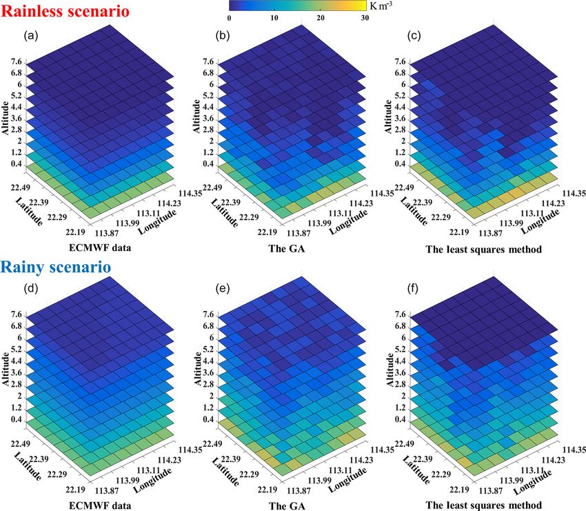
356                                                                    F. Yang et al.: A new water vapor tomography method

tions are GPS-derived slant water vapour data, the precip-         ner loop processes SWV by SWV and applies an adequate
itable water in the direction of the signal ray path, which        correction to each voxel. SWVs that execute the next itera-
travels through the troposphere from its top (Zhao and Yao,        tion start in the outer loop (Bender et al., 2011). Performing
2017). After obtaining the precise measurement of the sig-         the matrix inversion is not necessary, thus avoiding the ill-
nal ray distance in each voxel by ray tracing its path from        conditioned problem. However, only the results of the vox-
receiver to satellite, we can achieve the basic equation for       els that travelled through via signal rays are updated, and
water vapour tomography, which can be expressed in linear          the tomographic results heavily depend on the exact initial
form (Flores et al., 2000; Yang et al., 2018):                     field, the data quality and relaxation parameter (Wang et al.,
          n                                                        2014). Nilsson and Gradinarsky (2004) adapted a Kalman fil-
                 q                                                 ter approach to estimate tomographic results without adding
          X
SWVq =          di · x i ,                                  (1)
          i=1                                                      constraints and performing inversion. This approach assumes
                                                                   that the water vapour density in each voxel meets the Gauss–
where the superscript q is the satellite signal index, SWVq        Markov random walk pattern for a certain period of time, and
denotes the qth slant water vapour achieved by GPS tropo-          it establishes the corresponding state equation of the Kalman
spheric estimation and n is the total number of tomographic        filter. The observation vector used is based on the mathemat-
                      q
voxels discretized. di denotes the distance of the qth sig-        ical model to perform the optimal estimation of the state vec-
nal ray inside voxel i, which can be obtained by the satellite     tor, which is a process of continuous prediction and correc-
and station coordinates, and x i is the water vapour density of    tion. In this method, initializing the filter with an informed
voxel i. Using all suitable SWV observations, we can form          estimation of the water vapour field and providing the initial
the tomographic observation equation:                              covariance of state equation are based on external data. Other
y m×1 = Am×n · x n×1 ,                                      (2)    approaches that enrich the information of the observation
                                                                   equation were exploited in recent years, including the Con-
where y is a column vector of SWV, m is the total number of        stellation Observing System for Meteorology, Ionosphere,
SWV measurements in tomography, A denotes the intercept            and Climate (COSMIC) occultation data by Xia et al. (2013),
matrix containing the distance of the signal ray in each of        Interferometric Synthetic Aperture Radar (InSAR) by Bene-
the voxels, n is the number of voxels in the study area and x      vides et al. (2015), and water vapour radiometer (WVR) and
denotes the vector of the unknown water vapour density.            numerical weather prediction by Chen and Liu (2016).
   Since a GPS signal ray can only pass through a small part           In the above-mentioned tomographic methods, excessive
of the voxels in the study area, the elements of matrix A are      constraints on the matrix inversion, exact priori information
likely to be equal to zero, making it a large, sparse matrix. In   or external data are commonly used to overcome the ill-
addition, the effective signal rays will concentrate around the    conditioned problem. The mandatory usage of excessive con-
zenith due to the unfavourable geometry of the GPS stations        straints in tomographic experiments with poor voxel struc-
and the special structures of the satellites. These all make       ture will induce limitations, while reliance on exact priori in-
Eq. (2) ill conditioned, and it is difficult to obtain the un-     formation will make the tomographic solutions too similar to
knowns by performing the inversion of Eq. (2) in the form of       the priori data and decrease the role of the tomography tech-
x = A−1 · y.                                                       nique. External data cannot be used in all tomographic ex-
   To circumvent the ill-conditioned problem, many methods         periments. Therefore, this paper proposes a new tomography
are explored in the literature. Flores et al. (2000) added con-    method based on a genetic algorithm (Sect. 2). The tomogra-
straints on the vertical and horizontal variability of tomogra-    phy experiments and results of the analysis are presented in
phy with additional top constraints to the model. Most con-        Sect. 3. Section 4 summarizes the conclusions.
straints are based on experience and difficult to match to the
actual water vapour distribution, resulting in the deviation
of tomographic results. Moreover, singular value decompo-
sition (SVD) is required to perform matrix inversion. Bender       2     Methodology
et al. (2011) utilized an iterative algorithm called the alge-
braic reconstruction technique (ART) to solve the observa-         2.1     Troposphere estimation
tion equation. Several reconstruction algorithms of the ART
family were also implemented, e.g. the multiplicative alge-        In water vapour tomography, the observation is slant water
braic reconstruction techniques (MART) and the simultane-          vapour, which can be converted from slant wet delay (SWD)
ous iterations reconstruction technique (SIRT) (Stolle et al.,     by the following formula (Adavi and Mashhadi, 2015):
2006; Liu et al., 2010). The ART techniques are iterative al-
gorithms that proceed observation by observation. Only two         SWV = 5 × SWD
vectors, y and x, and a data structure containing the slant                                  106
sub-paths in each voxel are required to solve the observa-         =                                          × SWD,         (3)
                                                                                        k3
tion equations. The algorithms consist of two loops: The in-             ρw × mRw       Tm   + k2 − m w
                                                                                                    md × k1

Atmos. Meas. Tech., 13, 355–371, 2020                                                         www.atmos-meas-tech.net/13/355/2020/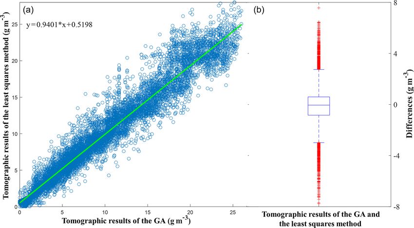
F. Yang et al.: A new water vapor tomography method                                                                            357

where 5 denotes a conversion factor. k1 = 77.604K hPa−1 ,          many years. The top constraint is obtained by setting the wa-
k2 = 70.4K hPa−1        and       k3 = 3.775 × 10⁵ K2 hPa−1 ;      ter vapour density of the top boundary to a small constant.
ρw is the liquid water density (unit: g m−3 ),                     Based on the principle of least squares, the tomographic re-
R = 8314 Pa m3 K−1 kmol−1         represents the univer-           sults can be achieved by the following formula:
sal gas constant, and mw = 18.02 kg kmol−1 and                                                      −1
md = 28.96 kg kmol−1 indicate the molar mass of wa-

                                                                   x = AT A + H T H + V T V + T T T    × AT y .                (9)
ter and the dry atmosphere, respectively. Tm denotes the
weighted mean temperature, which is the ratio of two vertical      To obtain the inverse matrix in Eq. (9), the singular value
integrals though the atmosphere (Davis et al., 1985). In prac-     decomposition is required. More details on this technique can
tice, an empirical formula is used to achieve approximate Tm       be found in Flores et al. (2000).
by surface temperature Ts in kelvin (Tm = 85.63 + 0.668 Ts )
(Liu et al., 2001; Astudillo et al., 2018). SWD can be             2.2   Water vapour tomography based on the genetic
obtained as follows (Zhang et al., 2017):                                algorithm
SWD = f (ele) × ZWD + f (ele) × cot (ele)
                                                                   For water vapour tomography based on the genetic algo-
× Gw                 w

   NS × cos (azi) + GWE × sin (azi) + Re ,                  (4)    rithm, the first procedure is to construct the tomographic
                                                                   equation. The idea of function optimization is then used to
where ele and azi are the satellite elevation and azimuth, re-
                                                                   solve Eq. (2) (Guo and Hu, 2009; Olinsky et al., 2004), which
spectively. f denotes the wet mapping function, Gw     NS and      is similar to the principle of least squares, V T PV = min (Flo-
GwWE  refer to the wet delay gradient parameters in the north–
                                                                   res et al., 2000). Equation (2) can be converted into the fol-
south and east–west directions, respectively. Re is the un-
                                                                   lowing form:
modelled atmospheric slant delay, which is included in the
zero-difference residuals. ZWD represents zenith wet delay,
                                                                   minf (x) = (y − Ax)T P (y − Ax) , x ∈ R+,                  (10)
which is the wet component of zenith total delay (ZTD) af-
fected by water vapour along the satellite signal ray. It can      where the terms are the same as in Eq. (2). In this equation,
be separated from ZTD by subtracting the zenith hydrostatic        the values of x that minimize function f (x) are the result
delay (ZHD). The ZTD is the primary parameter retrieved            of tomography. To achieve the best values of x, the tradi-
with GPS, and it is a spatially averaged parameter. If pres-       tional method adopts a derivative method which needs ma-
sure measurements are available, the ZHD is calculated by          trix inversion in the follow-up. The genetic algorithm, which
the Saastamoinen model as follows (Saastamoinen, 1972):            was first introduced by Holland (1992), provides an adap-
                   0.002277 × Ps                                   tive search method to achieve the tomographic results. It is
ZHD =                                        ,              (5)    designed to simulate the evolutionary processes in nature,
        1 − 0.00266 × cos (2ϕ) − 0.00028 × H
                                                                   in which the principle of survival of the fittest is applied
where Ps refers to the surface pressure, and ϕ and H rep-          to produce better and better approximates to the function.
resent the latitude and the geodetic height of the station, re-    Equation (10) is regarded as the fitness function that is used
spectively.                                                        to measure the performance of the searched values of x by
                                                                   computing the fitness value (Goldberg, 1989; Venkatesan et
2.1.1   Water vapour tomography based on the least
                                                                   al., 2004). Through searching generation after generation, the
        squares method
                                                                   water vapour result that best fits the function can be found.
After obtaining the observation equation (Eq. 2), three types      The specific steps of water vapour tomography based on the
of constraints are usually added:                                  genetic algorithm are as follows:

0 = H · x,                                                  (6)     1. construct the fitness function which is converted from
                                                                       the tomographic equation.
0 = V · x,                                                  (7)
0 = T · x.                                                  (8)     2. generate some groups representing approximates of x
                                                                       (water vapour density) stochastically, which form the
Equations (6)–(8) are the vertical, horizontal and top con-
                                                                       initial population,
straints, respectively. The horizontal constraint equation as-
sumes that the distribution of water vapour density is rela-        3. select groups from the last generation of the population
tively stable in the horizontal direction within a small region.       as parents according to a lower-to-higher order of the
Thus, the water vapour density within a certain voxel can              groups of x corresponding to their fitness values;
be represented by the weighted average of its neighbouring
voxels in the same layers. The vertical constraint equation is      4. produce offspring groups from parents by crossover and
a relationship established for the voxels between two adja-            mutation to make up a new set of approximated solu-
cent layers based on the analysis of meteorological data for           tions (new generation);

www.atmos-meas-tech.net/13/355/2020/                                                   Atmos. Meas. Tech., 13, 355–371, 2020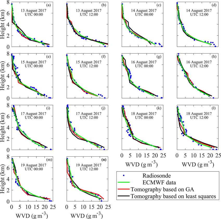
358                                                                      F. Yang et al.: A new water vapor tomography method

Figure 1. Flowchart of the water vapour tomography based on the genetic algorithm.

    5. compute the fitness values of the new generation, go           Table 1. Parameters of the genetic algorithm.
       back to step 3 and produce the next generation of the
       population;                                                        Parameter                          Strategy

    6. terminate the search when a group of approximates                  Population size                    200
                                                                          Crossover fraction                 0.8
       meets the requirements of the fitness value. (Generally,
                                                                          Reproduction of elite count        10
       we set the stopping criteria for generation or calculation         Selection function                 Roulette
       time.)                                                             Crossover function                 Intermediate
                                                                          Mutation function                  Adaptive feasibility
The parameters of genetic algorithm are listed in Table 1
                                                                          Generations of stopping criteria   100 × number of variables
(Wang et al., 2010). Roulette is a function used for selec-
tion in step 3, referring to the concept of a roulette wheel in
which the area of each segment is proportional to its expected
value, and one of the sections is selected with a random num-         region. The boundary and resolution in west–east and south–
ber whose probability equals its area. For the crossover func-        north directions were 113.87–114.35◦ and 0.06◦ and 22.19–
tion, “Intermediate” in Table 1 is intended to create offspring       22.54◦ and 0.05◦ , respectively; for the altitude direction, 0–
groups by a random weighted average of the parents. The               8.0 km and 800 m were chosen. A total of 8 × 7 × 10 voxels
mutation process forces the individuals in the population to          in the tomography grid was obtained. As shown in Fig. 2, 13
undergo small random changes that enable the genetic algo-            GPS stations of the Hong Kong Satellite Positioning Refer-
rithm to search a wider space. Adaptive feasibility is cho-           ence Station Network (green triangle) were selected in the
sen for the mutation function, which means that the adap-             tomography modelling to provide SWV measurements. An-
tive direction is generated randomly with respect to the last         other GPS station (KYC1, red spot) and radiosonde station
successful or unsuccessful generation (Dwivedi and Dikshit,           (45 005, blue spot) were used to check the result of tomog-
2013). Based on these steps, the optimal solution of Eq. (10)         raphy. Each GPS station recorded temperature, pressure and
is derived; that is, the value of x that gives f (x) the minimum      relative humidity by an automatic meteorological device, by
value, and also the value of water vapour density in the tomo-        which the hydrostatic parts of the troposphere delay can be
graphic equations. To more clearly show the process of water          accurately achieved. All the stations are under 400 m and lo-
vapour tomography based on a genetic algorithm, a flowchart           cated in the first layer of the tomographic grids.
is shown in Fig. 1.                                                      The GPS tropospheric parameters (zenith tropospheric de-
                                                                      lay and gradient parameters) were estimated by the GAMIT
3     Experiment and analysis                                         10.61 software based on a double-differenced model. In or-
                                                                      der to reduce the strong correlation of tropospheric param-
3.1    Experiment description                                         eters caused by the short baseline between GPS receivers
                                                                      in the tomographic area, three International GNSS Service
In order to conduct the tomographic experiment based on a             (IGS) stations (GJFS, LHAZ and SHAO) were incorporated
genetic algorithm, Hong Kong was selected as the research             into the solution model. In the processing, the sampling rate

Atmos. Meas. Tech., 13, 355–371, 2020                                                      www.atmos-meas-tech.net/13/355/2020/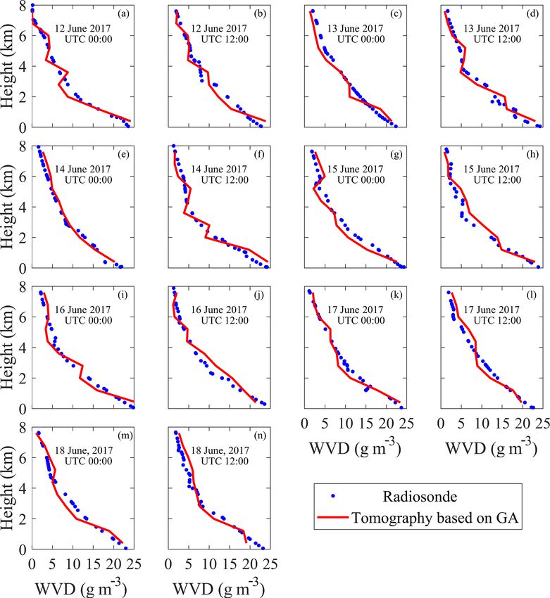
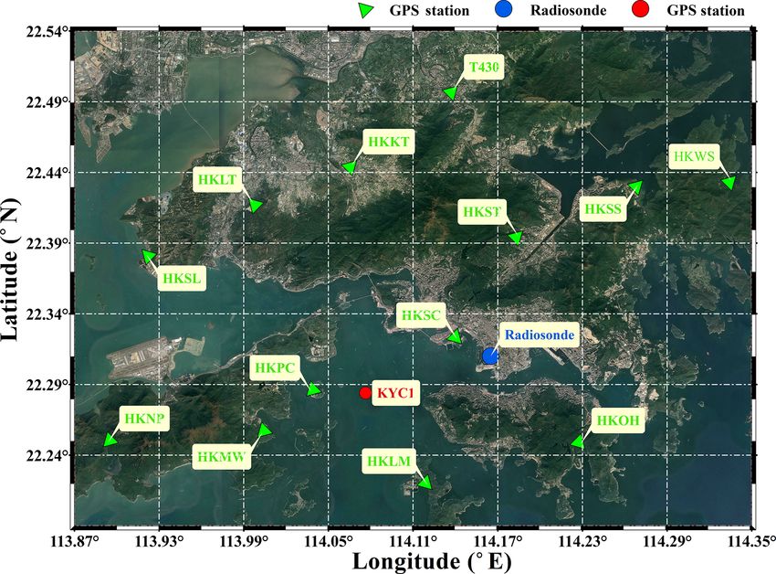
F. Yang et al.: A new water vapor tomography method                                                                                 359

Figure 2. Geographic distribution of GPS, radiosonde stations and the horizontal structure of the voxels used in water vapour tomography.
Map data ©2018 Google.

of observations was 30 s, a cut-off elevation angle of 10◦ was         rainless days. Hence, fine weather occurs without any rain-
selected, and the IGS precise ephemeris was adopted. The               fall. In addition, the relative humidity and SWV are small.
LC_AUTCLN and BASELINE modes were selected as the                      The other period is from 12 to 18 June 2017 (DOY of 163
processing strategies, meaning that the GPS observation was            to 169, 2017), which covers the rainy days. During the se-
the ionosphere-free linear combination and the orbital pa-             lected rainy period, the weather of Hong Kong was first af-
rameters were fixed, respectively. The tropospheric param-             fected by the approach and the passage of a severe tropical
eters, including troposphere delay gradients and ZTD at 4              storm, named Merbok, with more than 150 mm of rainfall
and 2 h intervals, are estimated and interpolated to a 30 s            recorded on 13–14 June. Thereafter, from 15 and 16 June,
sampling rate in the GAMIT software. Note that the out-                the influence of an enhanced southwest monsoon and the de-
puts of GAMIT are double-differenced residuals and tropo-              velopment of a lingering through of low pressure made the
sphere delay gradients. To obtain the R in Eq. (4), double-            remaining weather unstable and rainy till 21 June. In this pe-
differenced residuals should be converted to zero-difference           riod of time, the maximum daily rainfall is up to 203.7 mm,
residuals, and multipath effects should be considered by the           and the average daily rainfall is 66.8 mm. The average rel-
method proposed by Alber et al. (2000). To achieve the wet             ative humidity and SWV produced in the selected stations
delay gradients, Bar-Sever et al. (1998) considered the av-            are 89 % and 112.9 mm, respectively. This period represents
erage of troposphere gradients within 12 h as the dry delay            rainy days, indicating that continuous rainfall occurs, and the
gradients and subtracted it from the troposphere delay gra-            relative humidity and SWV are high. The period covered is
dients. Then all the necessary parameters are available for            0.5 h for each tomographic solution. The radiosonde data,
Eq. (4) to build SWD, and SWV was obtained by Eq. (3).                 collected twice daily at 00:00 and 12:00 UTC in these two
   To verify the proposed method, two periods of GPS obser-            periods, were treated as reference data.
vation data, with a sampling rate of 30 s, were used in the               According to the flowchart presented in Fig. 1, the above
tomography experiment. One from 13 to 19 August 2017                   GPS observation data were processed to construct the tomo-
(day of year (DOY) of 225 to 231, 2017), during which a                graphic equation and further converted into the fitness func-
spell of fine weather prevailed in Hong Kong with a ridge of           tion for the optimization algorithm. Population size is cho-
high pressure extending westwards from the Pacific to cover            sen based on the total number of unknown parameters (water
south-eastern China on 16–18 August. In that period of time,           vapour density). The value of 200 is the default option of the
the daily rainfall was 0 mm. Moreover, the relative humid-             algorithm when the number of unknowns exceeds a certain
ity and SWV produced in the selected stations on average               amount. The reproduction of elite count is chosen to be 10 to
are 75 % and 79.1 mm, respectively. This period is defined as          specify the number of individuals that are guaranteed to sur-

www.atmos-meas-tech.net/13/355/2020/                                                        Atmos. Meas. Tech., 13, 355–371, 2020
360                                                                          F. Yang et al.: A new water vapor tomography method

Figure 3. Grayscale graph of number of signal rays passing through each voxel and distribution of voxel with sufficient signal rays (a, b stand
for a rainless and a rainy day, respectively).

vive to the next generation because it is based on population             3.2   Analysis of matrix ill condition
size (0.05 × population size). The crossover fraction is set to
the default value of 0.8 to specify the fraction of the next
generation that crossover produces. In this study, generation             In a tomographic solution, the structure of the coefficient ma-
is chosen as the stopping criteria and “100 × number of vari-             trix in the observation equation depends on which voxels are
ables” is the default. Other parameters, including roulette, in-          crossed by SWV and the number of signal rays penetrating
termediate and adaptive feasibility, are selected because they            each voxel. Figure 3 illustrates this in the form of a grayscale
are the most commonly used settings for genetic algorithms.               graph for two different days: 13 August 2017 at 00:00 UTC,
Other selection functions as well as crossover and mutation               a rainless day (a), and 13 June 2017 at 12:00 UTC, a rainy
functions can be adopted in the genetic algorithm. In ad-                 day (b). In the upper panels of each sub-figure, the deepen-
dition, population size, crossover fraction, elite count and              ing of the grayscale refers to an increase in the number of
stopping criteria can also be set to other values which may               signal rays crossing through the voxel. The closer the layer
slightly affect solution time and results. The specific impact            is to the ground, the more voxels are not crossed by any sig-
can be explored in depth in future research.                              nal rays. Although there are few voxels with no signal rays
                                                                          passing through in the upper layers, many of the voxels have

Atmos. Meas. Tech., 13, 355–371, 2020                                                          www.atmos-meas-tech.net/13/355/2020/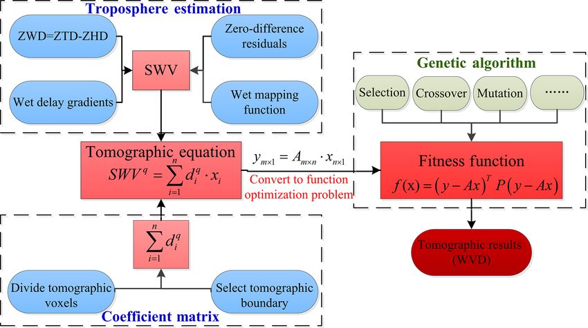
F. Yang et al.: A new water vapor tomography method                                                                                  361

Figure 4. Scatter diagram of the SWV residuals in different weather conditions for internal accuracy testing.

a lighter grayscale, which means that the voxels are crossed             water vapour tomographic observation equation established
by fewer signal rays.                                                    in Eq. (1). In this process, the parameters on the right side
   Note that when the signal ray passes vertically through the           of Eq. (1) (the distance of the signal ray in each of the
tomographic region, the ray crossed a minimum number of                  voxels and the water vapour density calculated by the to-
voxels; that is, 10 in the tomographic area. Therefore, the              mographic modelling) are taken as known quantities. More-
minimum probability that a voxel will be crossed by a ray                over, the SWV on the left is the parameter to be determined,
is 1.79 % (10/560; 560 is the total number of voxels in this             i.e. the tomography-computed SWV. The differences against
tomographic experiment). Thus 1.79 % of the total SWV is                 the GAMIT-estimated SWV (as a reference) were also iden-
taken as a criteria to further illustrate the structure of the co-       tified.
efficient matrix. If the number is greater than the threshold,               For internal accuracy testing, 13 GPS stations used in the
the voxel is considered to be crossed by sufficient rays, oth-           tomographic modelling were adopted. The change of tomog-
erwise the voxel is defined as an insufficient one. For the two          raphy computed vs. GAMIT-estimated slant water vapour
examples shown, the number of total SWV and the criteria                 residuals with elevation angle is shown in Fig. 4, where the
are 4930/4569 and 88/81, respectively. The lower panels of               blue and red dots represent the rainy and rainless days, re-
each sub-figure display the distribution of sufficient (black            spectively. The maximum residuals for rainy and rainless
rectangle) and insufficient (white rectangle) ones. Obviously,           scenarios are 10.74 and −9.84 mm, respectively. The root
many voxels are not crossed by enough satellite rays, both for           mean square error (RMSE) and mean absolute error (MAE)
the upper layers or the lower layers.                                    for rainy and rainless days are 1.56/0.98 and 1.48/0.89 mm,
   To better analyse the ill-conditioned nature of the observa-          respectively. Figure 4 shows that most of the residuals are
tion equation in tomography modelling, the number of zero                concentrated between −2.0 and 2.0 mm, which indicates
elements in matrix A is counted. We found that the propor-               good internal accuracy.
tion of zero element is over 97 % in all tomographic solu-                   To normalize SWV residuals for their evaluation in a
tions. In addition, the concept of matrix condition number is            single unit, we mapped the tomography-computed SWVs
introduced to measure the degree of dispersion of the eigen-             back to the zenith direction using the 1/ sin(e) formula and
values of the coefficient matrix (Edelman, 1989). The larger             computed their differences with the GAMIT-estimated SWV
the value of the condition number, the more ill-conditioned              (Michal et al., 2017). Figure 5 shows the statistical results of
the matrix is. The results show that the condition number in             the residuals in the zenith direction. In the figure, the colours
every tomographic solution is infinite, which means a serious            indicate the weather conditions (blue for rainy days and red
ill-conditioned problem.                                                 for rainless days), and the 13 stations were arranged in the
                                                                         order in which they were added to the tomographic model.
3.3   Internal accuracy testing                                          The maximum and minimum RMSE in the two periods are
                                                                         0.79 and 1.81 mm, respectively, whereas the maximum and
To evaluate the performance of water vapour tomography                   the minimum values for MAE are 0.43 and 1.54 mm, respec-
based on a genetic algorithm, slant water vapour of GPS sta-             tively. The RMSE and MAE of rainless days are better than
tions for the data of 13 to 19 August and 12 to 18 June 2017             those of rainy days in each station. The medians of RMSE
were computed using the tomographic results based on the

www.atmos-meas-tech.net/13/355/2020/                                                          Atmos. Meas. Tech., 13, 355–371, 2020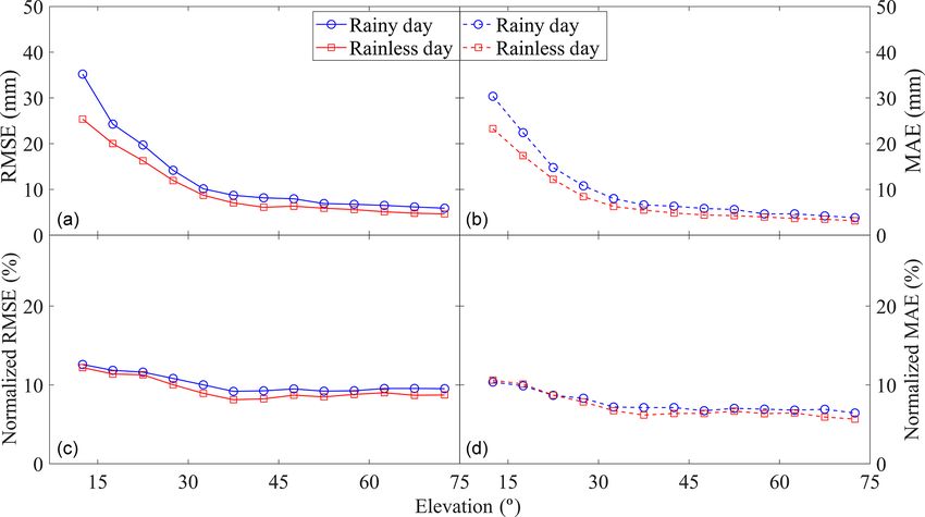
362                                                                     F. Yang et al.: A new water vapor tomography method

Figure 5. Comparison of SWV residuals in zenith direction: circles for RMSE and diamonds for MAE; blue for rainy days and red for
rainless days.

                                                                      Figure 7. Comparison of SWV residuals (differences between the
Figure 6. Histogram for MAE (a) and RMSE (b) of SWV residuals
                                                                      tomography-computed SWV and GAMIT-estimated SWV) for the
(differences between the tomography-computed SWV and GAMIT-
                                                                      KYC1 station in each elevation bin; (a,b) for RMSE / MAE; (c, d)
estimated SWV) for the KYC1 station, which has not been used
                                                                      for normalized RMSE / MAE.
in the tomographic modelling (blue for rainy days, red for rainless
days).

and MAE are displayed for 13 stations to highlight differ-            3.4   External accuracy testing
ences among the stations. A particular outlier is the HKMW
station, with RMSE and MAE values of 1.81/1.53 and                    For external accuracy testing, the data from KYC1 station,
1.60/1.23 mm in rainy and rainless days, respectively. The            which was not included in the tomographic modelling, were
reason for the divergent behaviour may be that two stations           used. Figure 6 shows the histogram for MAE (upper) and
(HKPC and HKMW) exist in the same voxel, which may                    RMSE (lower) of SWV residuals (differences between the
result in the station (HKPC) data first introduced into the to-       tomography-computed SWV and GAMIT-estimated SWV),
mographic model affecting the subsequent station (HKMW)               in which the blue and red bars represent rainy and rainless
data. This hypothesis will be further investigated in future          days, respectively. The dashed bars are the averages for those
research. However, plots with RMSE and MAE are consis-                different weather conditions. From this figure, it can be noted
tent within 2.0 mm among all the stations (1.5 mm except for          that all MAE and RMSE values are below 15 mm, with av-
HKMW).                                                                erage values lower for rainless days than for rainy days, re-
                                                                      spectively 8.75/7.33 and 11.38/9.54 mm for RMSE / MAE.
                                                                      Therefore, a good external accuracy is achieved by tomo-
                                                                      graphic solutions, considering the low RMSE and MAE of
                                                                      rainy and rainless days.

Atmos. Meas. Tech., 13, 355–371, 2020                                                    www.atmos-meas-tech.net/13/355/2020/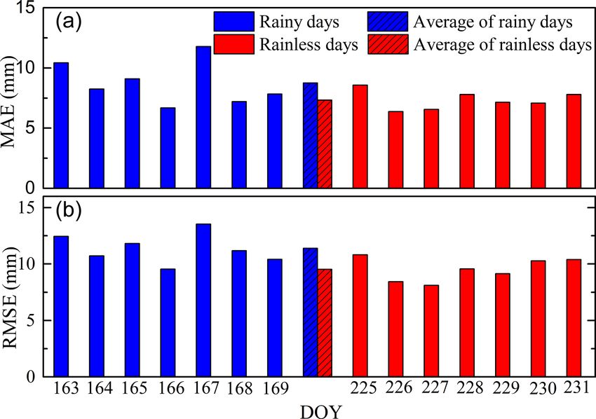
F. Yang et al.: A new water vapor tomography method 363
the box plots. Q1 and Q3 located at the bottom and top of the
box represent the first and third quartiles; the second quar-
tile (Q2) is located inside the box; the ends of the whiskers
refer to the upper and lower bounds, which are located at
Q1 − 1.5 (IQR) and Q3 + 1.5 (IQR), respectively. IQR is the
interquartile range, defined as the difference between Q3 and
Q1, and it reflects the discreteness of a set of data. In Fig. 8
the length of the box and the range of bound in rainless days
(in red) are smaller than those in rainy days (in blue), indicat-
ing better residual distribution in rainless days than in rainy
days. The right plot (in green) denotes the result of the com-
bination of rainless and rainy days, representing the overall
distribution of SWV residuals of tomography based on a ge-
netic algorithm. In our experiments, 50 % of the residuals are
concentrated between −7.08 and 4.47 mm and only 3.24 %
of the residuals are outliers when combining the data of rainy
and rainless days.
Figure 8. Box plots of the SWV residuals (differences between the
tomography-computed SWV and the GAMIT-estimated SWV) for 3.5 Comparison with radiosonde data
the KYC1 station.
The water vapour density profile derived from the radiosonde
data can be used as a reference value, which is well suited to
To further assess external accuracy, slant water vapour out- evaluate the accuracy of the tomographic results based on
puts were grouped into individual elevation bins of 5◦ , i.e. all a genetic algorithm. As the radiosondes are launched daily
SWVs with an elevation angle between 10 and 15◦ were eval- at 00:00 and 12:00 UTC, the tomographic results of 12 to
uated as a single unit. The RMSE and MAE of each elevation 18 June (rainy days) and 13 to 19 August 2017 (rainless
bin were calculated. To examine the dependence of relative days) at these times were compared. Figure 9 shows the wa-
errors in SWVs at different elevations, normalized RMSE ter vapour density comparisons between radiosonde data and
and MAE were computed. For this computation, residuals of tomographic results for different altitudes at individual dates
SWV were divided by the GAMIT-estimated SWV and mul- (rainy period). It is clear from the profiles that the water
tiplied by 100 to obtain the percentages. Figure 7 shows the vapour density (WVD) decreases with increasing height. The
variation of RMSE, MAE, normalized RMSE and normal- WVD profiles reconstructed by the GA tomographic solu-
ized MAE as the elevation angle changes in different weather tions conform with those derived from the radiosonde data,
conditions. For Fig. 7a and b, the RMSE and MAE reduc- especially in the upper troposphere in absolute terms. With
tion of SWV residuals are clearly visible as the increasing respect to the relative error, the values of the voxels higher
elevation angle, which is consistent with the trend shown in than 5 km and lower than 5 km are 31 % and 15 %, respec-
Fig. 4. The colours in the figure indicate that better RMSE tively. The reason for this phenomenon is that the value of
and MAE results can be achieved on a rainless day than on water vapour in the upper layers is relatively low. Even a
a rainy day in each elevation bin. In terms of normalized small difference between the radiosonde and tomographic re-
RMSE and MAE, we note that they remain almost constant sult can also lead to a large relative error, whereas the water
over all elevation angles, indicating a consistent relative per- vapour content resides for more than 90 % below 5 km near
formance of computing SWV in each type of weather con- the Earth’s surface. In certain cases, a relatively good consis-
dition. It is noted that the normalized RMSE and MAE of tency can also be seen in the lower atmosphere. This may be
rainless days are close to those of rainy days which may be because a GPS station (HKSC) for tomography modelling is
due to the large SWV during rainy days that introduced a located at the voxel where the radiosonde station is situated,
large denominator in the normalized calculation. Therefore, resulting in the low atmosphere with sufficient signal rays
the good performance on relative error in SWVs at different passing through.
elevations with a low normalized RMSE / MAE (< 0.125 for To further illustrate the comparison with the radiosonde
normalized RMSE and < 0.106 for normalized MAE) points data, Table 2 lists RMSE and MAE of the WVD. In the
to good external accuracy. table, the WVD in the voxels above the radiosonde station
In the above analysis, RMSE and MAE were used for the computed by tomography and those derived from radiosonde
external accuracy testing of the tomographic results based on are counted to calculate their RMSE and MAE in each so-
the GA. Box plots are used to explore the statistical charac- lution. Thus, the average RMSE / MAE of rainless days are
teristics of SWV residuals and to detect the outliers in the 1.35/1.08 g m−3 , which is smaller than 1.51/1.29 g m−3 in
tomographic errors. Five characteristic values are shown in rainy days. This finding is consistent with the comparison of
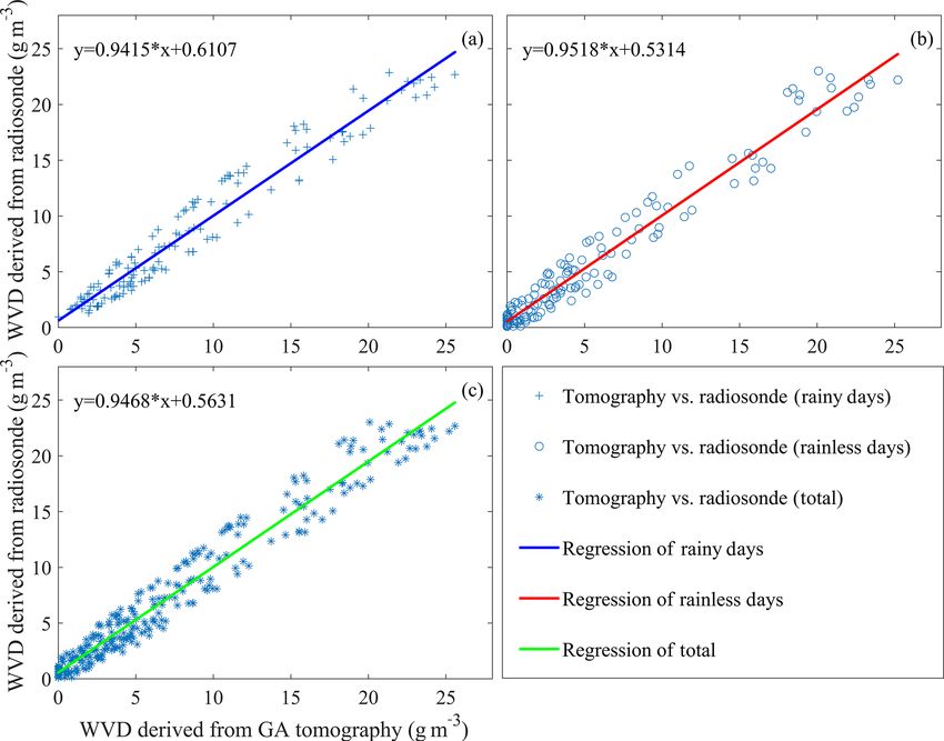
www.atmos-meas-tech.net/13/355/2020/ Atmos. Meas. Tech., 13, 355–371, 2020364 F. Yang et al.: A new water vapor tomography method Figure 9. Panels (a)–(n) represent water vapour density comparisons between radiosonde and tomography based on the genetic algorithm at 00:00 and 12:00 UTC from 12 to 18 June 2017 (rainy days). SWV above. We compare those values with the results ob- for the two time periods in this paper can be considered to tained from other Hong Kong tomographic experiments. For be in good agreement with the radiosonde data regardless example, Xia et al. (2013) obtained an RMSE of 1.01 g m−3 of the weather conditions. Moreover, many different settings by adding the COSMIC profiles as external data based on are applied in tomographic experiments by different groups, a two-step reconstruction. Using the least squares method such as the selection of tomographic boundary, differences in with horizontal and vertical constraints, Yao et al. (2016) ob- experimental period and weather conditions, division rule of tained an RMSE of 1.23 g m−3 by maximally using GPS ob- horizontal and vertical voxel, and addition of other observa- servations and an RMSE of 1.60 g m−3 without the operation. tions. Zhao et al. (2017) achieved an RMSE of 1.19 and 1.61 g m−3 To explore the overall accuracy of water vapour density considering the signal rays crossing from the side of the re- reconstructed by the GA tomography, the linear regression search area and an RMSE of 1.79 g m−3 without this con- analysis and box plot were adopted for different weather sideration. Yao et al. (2017) achieved an RMSE from 1.48 to conditions. Figure 10 shows the linear regression of the wa- 1.80 g m−3 using different voxel division approaches. Ding et ter vapour density for rainy days (Fig. 10a), rainless days al. (2017) obtained an RMSE of 1.23 g m−3 by utilizing the (Fig. 10b) and their combination (Fig. 10c), in which the new parametric methods based on inverse-distance-weighted scatter points of three graphs are close to the 1 : 1 lines. In (IDW) interpolation and an RMSE of 1.45 g m−3 using the comparison with the coefficients of regression equations, the traditional methods, respectively. Note that the RMSE val- results from rainless days are slightly better than those of ues calculated in the above experiments are based on the rainy days. When combining the data of two periods, the radiosonde data. Therefore, the total RMSE of 1.43 g m−3 starting point of the regression equation is 0.5631 and the Atmos. Meas. Tech., 13, 355–371, 2020 www.atmos-meas-tech.net/13/355/2020/
F. Yang et al.: A new water vapor tomography method                                                                               365

Figure 10. Linear regression of the water vapour density from radiosonde and tomography based on the genetic algorithm. Panels (a), (b)
and (c) represent rainy days, rainless days and their combination, respectively.

Table 2. RMSE and MAE of the water vapour density comparison between radiosonde and tomography based on the genetic algorithm for
different weather conditions (g m−3 ).

                          Weather         Date                   RMSE                        MAE
                          condition                    00:00 UTC     12:00 UTC     00:00 UTC     12:00 UTC
                          Rainy days      12 June             1.54          1.68          1.27          1.43
                                          13 June             1.20          1.57          1.81          1.39
                                          14 June             1.37          1.79          0.85          1.56
                                          15 June             1.63          1.38          1.41          1.27
                                          16 June             1.77          1.48          1.56          1.31
                                          17 June             1.49          1.33          1.55          1.18
                                          18 June             1.52          1.38          1.34          1.22
                                          Average                 1.51                        1.29
                          Rainless days   13 August           1.44          1.35          1.14          0.93
                                          14 August           1.46          1.25          1.18          1.05
                                          15 August           1.54          1.27          1.26          0.83
                                          16 August           1.29          1.14          1.03          0.89
                                          17 August           1.38          1.39          1.09          1.24
                                          18 August           1.46          1.26          1.19          1.06
                                          19 August           1.23          1.40          1.03          1.19
                                          Average                 1.35                        1.08
                          Total                                   1.43                        1.19

www.atmos-meas-tech.net/13/355/2020/                                                       Atmos. Meas. Tech., 13, 355–371, 2020
366 F. Yang et al.: A new water vapor tomography method
Table 3. Statistical results of the GA and the least squares method
comparison; ECMWF data are shown as a reference (g m−3 ).
GA method Least squares
method
RMSE MAE RMSE MAE
Rainy scenario 1.84 1.42 1.94 1.47
Rainless scenario 1.71 1.39 1.79 1.37
Average 1.78 1.41 1.87 1.42
(the GA and the least squares) generally have a good con-
sistency with ECMWF data regardless of the weather condi-
tions, and they can accurately describe the spatial distribu-
tion of water vapour. Additionally, a larger variation of water
Figure 11. Box plots of the WVD residuals, which are computed vapour with altitude occurs in a rainy scenario than in a rain-
between the GA tomographic approach and radiosondes. less scenario, especially in the upper atmosphere, which is
well captured by the GA and the least squares method. Nu-
merical results including RMSE and MAE during the whole
slope is 0.9468; water vapour density can be achieved with experimental period are listed in Table 3 to show the com-
high accuracy by tomography based on the GA. The corre- parison of the GA and the least squares method, in which the
sponding box plots are shown in Fig. 11. It can be noted that water vapour density derived from ECMWF data is regarded
the WVD residuals are concentrated in the range of −2 to as the true value. It indicates that the result of the GA is a
2 mm, and the rainless scenario is better than the rainy sce- little better than that of the least squares method.
nario. The Q1 / Q3 values are −1.28/1.08, −1.20/0.65 and To further analyse the tomographic results of the GA
−1.24/0.87 mm for rainy days, rainless days and their com- and the least squares method, regression and boxplot anal-
bination, respectively. The upper and lower boundaries are yses are conducted and displayed in Fig. 13, which cov-
located near 4 and −4 mm. No outlier is present in this box ers all solutions, each of them containing 560 voxel re-
plots, probably due to few WVD residuals. sults. In Fig. 13a, a good linear regression relationship is
shown by the distribution of scatter points and the straight
3.6 Comparison with tomographic results of the least line of regression. Specifically, the starting points of the re-
squares method gression equation and the slope are 0.5198 and 0.9401, re-
spectively. The right panel shows the distribution of differ-
The least squares method is most commonly used in wa- ences between the two types of tomographic results. The
ter vapour tomography, and numerous experiments prove Q1 and Q3 are −0.84 and 0.60 g m−3 , respectively, which
that water vapour density with high accuracy can be ob- means that more than 50 % of the differences between the
tained with this method (Flores, et al., 2000; Zhang et al., two methods are within 1 g m−3 . The upper and lower bounds
2017; Zhao et at., 2017). To verify the accuracy of the ge- are 2.75 and −2.98 g m−3 , respectively, and outliers only
netic algorithm, we compared the tomographic results be- account for 3.11 %. Consequently, the tomographic results
tween the genetic algorithm and the least squares method based on the GA are in agreement with those of the least
in this section. The specific process and introduction to the squares method for this experiment. A reliable tomographic
least squares method can be found in detail in Flores et result can be achieved by the GA without being restricted by
al. (2000), Guo et al. (2016) and Yang et al. (2018). Fig- constraint equations and matrix inversion like the traditional
ure 12 shows the three-dimensional distribution of water least squares method.
vapour density derived from tomography based on the GA Moreover, a detailed comparison between GA and the
and the least squares method. The water vapour computed by least squares method is conducted using the voxels above
the European Centre for Medium-Range Weather Forecasts the radiosonde station. Figure 14 shows the changes in wa-
(ECMWF) data, which provides various meteorological pa- ter vapour density derived from GA and the least squares
rameters at different pressure levels with a spatial resolution method with altitudes in different days (rainless days), in
of 0.125◦ × 0.125◦ , is displayed in the figure as a reference. which the radiosonde data and ECMWF data are considered
Here both the GA and the least squares method give a reason- reference data. All the profiles derived from the two methods
able tomographic result. In certain voxels, the GA achieves decrease with increasing height and show good consistency
the closer results to the ECMWF data, whereas for other vox- with the reference data. The statistical values are computed
els, the least squares method performs better. Both methods and listed in Table 4 to illustrate the comparison of GA and
Atmos. Meas. Tech., 13, 355–371, 2020 www.atmos-meas-tech.net/13/355/2020/F. Yang et al.: A new water vapor tomography method 367 Figure 12. The three-dimensional distribution of water vapour density derived from ECMWF data, the GA method and the least squares method (upper for rainless scenario and lower for rainy scenario). Figure 13. Regression (a) and boxplot (b) for tomographic results (WVD) of the GA and the least squares method. www.atmos-meas-tech.net/13/355/2020/ Atmos. Meas. Tech., 13, 355–371, 2020
368                                                                     F. Yang et al.: A new water vapor tomography method

Figure 14. Water vapour density comparisons between GA and the least squares method in the selected voxels at 00:00 and 12:00 UTC from
13 to 19 August 2017 (rainless days); radiosonde and ECMWF data are used as reference.

the least squares method. The RMSE and MAE indicate that             ties along the radiosonde path were collected during the ex-
both the GA and the least squares method can achieve good            periments. Their changes with altitude are shown in Fig. 15,
tomographic results compared with the reference values (ra-          in which the rainy and rainless weather are represented by
diosonde and ECMWF data) whether in the rainy or rainless            blue and red dots, respectively. The situation of 8–12 km is
scenario. The GA which has an average RMSE / MAE of                  magnified to show the water vapour information outside the
1.43/1.19 and 1.30/1.05 g m−3 compared with radiosonde               tomographic region. In the figure, the larger value of WVD
and ECMWF data, respectively, performs slightly better than          can be observed above 8 km in rainy days compared with that
the least squares method, of which the average RMSE / MAE            of rainless days. For the rainless situation, the value of WVD
are 1.49/1.23 and 1.36/1.12 g m−3 .                                  within 8–12 km is small and near to zero. By contrast, the
                                                                     value is basically not close to zero in the rainy situation, espe-
3.7   Analysis of results in different weather conditions            cially in the range of 8–10 km, which is substantially greater
                                                                     than 0.5 g m−3 . Referring to the selection of the tomographic
In our experiments, the comparisons under various weather            heights in other articles, considering the long-term statistics
conditions illustrate that the tomographic result of rainless        of water vapour in Hong Kong, and taking into account the
scenarios was better than rainy scenarios, which is also con-        drawbacks of the excessive number of tomographic voxels,
cluded in other studies (Yao et al., 2016; Zhao et al., 2017;        we selected 8 km as the top boundary of the research area in
Ding et al., 2017). This result is because the spatial struc-        this paper, which ignores the water vapour information above
ture of atmospheric water vapour is relatively stable in rain-       8 km in our tomographic model. Obviously, it has limited in-
less weather, whereas its spatial distribution changes faster        fluence on the accuracy of the tomographic result in rainless
in rainy weather. Thus, certain limitations are imposed on to-       weather condition. For the rainy weather condition, the ef-
mography to obtain accurate water vapour during unstable             fect could be slightly larger, which is one reason why the
weather conditions. Additionally, all the water vapour densi-

Atmos. Meas. Tech., 13, 355–371, 2020                                                    www.atmos-meas-tech.net/13/355/2020/
F. Yang et al.: A new water vapor tomography method 369
Table 4. Statistical results of the GA and the least squares method using radiosonde and ECMWF data as reference in the selected voxels
(g m−3 ).
Data comparison Rainy days Rainless days Average
RMSE MAE RMSE MAE RMSE MAE
Radiosonde vs. GA 1.51 1.29 1.35 1.08 1.43 1.19
Radiosonde vs. least squares method 1.58 1.34 1.40 1.16 1.49 1.25
ECMWF vs. GA 1.35 1.12 1.25 0.97 1.30 1.05
ECMWF vs. least squares method 1.43 1.20 1.29 1.03 1.36 1.12
rithm through the process of selection, crossover and muta-
tion.
Our new approach is validated by tomographic experi-
ments using GPS data collected over Hong Kong from 12
to 18 June (rainy days) and 13 to 19 August 2017 (rain-
less days). The problem of matrix ill condition was dis-
cussed and analysed by the grayscale graph and condition
number. In a comparison of the SWV residuals, internal and
external accuracy testing were used for the GA tomogra-
phy. The internal accuracy testing refers to computing the
differences between the tomography-computed SWV and
GAMIT-estimated SWV for the 13 GPS stations used in the
tomographic modelling, whereas the external accuracy test-
ing denotes the differences for the KYC1 station which is not
included in the tomographic modelling. The RMSE / MAE
of SWV residuals are 1.52/0.94 and 10.07/8.44 mm for the
internal and external accuracy testing, respectively. Thus, a
good tomographic result is achieved. In addition, the water
Figure 15. Changes in water vapour density with altitude in dif- vapour density of the proposed method agreed with that of
ferent weather conditions; data are from radiosonde measurements radiosonde. The RMSE and MAE are 1.43 and 1.19 g m−3 ,
(blue for rainy days from 12 to 18 June 2017 and red for rainless whereas the starting point and the slope of the regression
days from 13 to 19 August 2017). equation are 0.5631 and 0.9468, respectively. ECMWF data
are utilized to display the three-dimensional distribution of
tomographic results. The least squares method is selected as
tomographic results of rainy days were worse than those of the representative of the traditional tomographic method to
rainless days in our experiments. compare with the GA. A good consistency is demonstrated in
terms of RMSE, MAE, linear regression and boxplot. Thus, a
reliable tomographic result can be achieved by the GA with-
4 Conclusions out being restricted by constraint equations and matrix in-
version like the traditional least squares method. Moreover,
In this paper, a new tomography approach based on the the comparison under various weather conditions illustrated
genetic algorithm was proposed to reconstruct a three- that the tomographic result of the rainless scenario was bet-
dimensional water vapour field in Hong Kong under rainy ter than that of the rainy scenario, and the reasons were dis-
and rainless weather conditions. The inversion problem was cussed. In a future study, the tomography approach based on
transformed into an optimization problem that no longer de- the genetic algorithm, which is not dependent on constraints,
pends on excessive constraints, a priori information or exter- a priori data and external data, could provide potential in-
nal data. Thus, many problems do not need to be considered, terest for the establishment of a real-time or near-real-time
including the difficulty of inverting the sparse matrix, the water vapour tomographic system.
limitation and irrationality of constraints, the weakening of
tomographic technique by prior information, and the restric-
tion of obtaining external data. Based on the fitness function
established by the tomographic equation, the water vapour
tomographic solution could be achieved by the genetic algo-
www.atmos-meas-tech.net/13/355/2020/ Atmos. Meas. Tech., 13, 355–371, 2020370 F. Yang et al.: A new water vapor tomography method
Data availability. The GNSS observations and the relative meteo- Bar-Sever, Y. E., Kroger, P. M., and Borjesson, J. A.: Estimat-
rological data can be download from the Hong Kong Satellite Posi- ing horizontal gradients of tropospheric path delay with a sin-
tioning Reference Station Network (SatRef) (https://www.geodetic. gle GPS receiver, J. Geophys. Res.-Sol. Ea., 103, 5019–5035,
gov.hk/en/satref/satref.htm, last access: 20 February 2019). The ra- https://doi.org/10.1029/97JB03534, 1998.
diosonde data of Hong Kong were obtained from the Department Bender, M., Dick, G., Ge, M., Deng, Z., Wicker, J., Kahle,
of Atmospheric Science, University of Wyoming (http://weather. H.-G., Raabe, A., and Tetzlaff, G.: Development of a
uwyo.edu/upperair/sounding.html, last access: 20 February 2019). GNSS water vapor tomography system using algebraic re-
The ECMWF data are available from the European Centre for construction techniques, Adv. Space Res., 47, 1704–1720,
Medium-Range Weather Forecasts (http://apps.ecmwf.int/datasets/, https://doi.org/10.1016/j.asr.2010.05.034, 2011.
last access: 20 February 2019). Benevides, P., Nico, G., and Catalao, J.: Merging SAR interferom-
etry and GPS tomography for high-resolution mapping of 3-D
tropospheric water vapor, In Proceedings of the Geoscience and
Author contributions. FY, JG and JS did the conceptualization; YZ, Remote Sensing Symposium, Milan, Italy, 26–31 July 2015.
LZ and DZ conducted the data curation; FY, JG and JS conducted Bevis, M., Businger, S., Herring, T. A., Rocken, C., An-
the formal analysis; FY proposed the methodology; JS and XM thes, R. A., and Ware, R. H.: GPS meteorology: Remote
provided the resources; FY validated the experimental results; FY sensing of atmospheric water vapor using the Global Posi-
wrote the original draft; FY, JG, XM, JS, LZ, YZ and DZ reviewed tioning System, J. Geophys. Res.-Atmos., 97, 15787–15801,
and edited the manuscript. https://doi.org/10.1029/92JD01517, 1992.
Braun, J., Rocken, C., Meetrens, C., and Ware, R.: Development
of a Water Vapor Tomography System Using Low Cost L1 GPS
Competing interests. The authors declare that they have no conflict Receivers, 9th ARM Science Team Meeting, US Dep. of Energy,
of interest. San Antonio, Texas, 22–26 March 1999.
Chen, B. and Liu, Z.: Assessing the performance of troposphere to-
mographic modeling using multi-source water vapor data during
Hong Kong’s rainy season from May to October 2013, Atmos.
Acknowledgements. The authors would like to thank the Lands De-
Meas. Tech., 9, 5249–5263, https://doi.org/10.5194/amt-9-5249-
partment of HKSAR for providing the GNSS data from the Hong
2016, 2016.
Kong Satellite Positioning Reference Station Network (SatRef).
Davis, J., Herring, T., Shapiro, II., Rogers, A., and Elgered, G.:
Chinese Scholarship Council (CSC) and the University of Notting-
Geodesy by radio interferometry: Effects of atmospheric model-
ham for providing the opportunity for the first author to study at the
ing errors on estimates of baseline length, Radio Sci., 20, 1593–
University of Nottingham for 1 year. Acknowledgements are also
1607, https://doi.org/10.1029/RS020i006p01593, 1985.
given to the editor in charge (Roeland Van Malderen) and my col-
Ding, N., Zhang, S., and Zhang, Q.: New parameterized model
league at the University of Nottingham (Simon Roberts) for their
for GPS water vapor tomography, Ann. Geophys., 35, 311–323,
revision to improve the English language and style of the paper.
https://doi.org/10.5194/angeo-35-311-2017, 2017.
Dong, Z. and Jin, S.: 3-D water vapor tomography in Wuhan from
GPS, BDS and GLONASS observations, Remote Sens., 10, 62,
Financial support. This research has been supported by the Na- https://doi.org/10.3390/rs10010062, 2018.
tional Natural Science Foundation of China (grant nos. 41474004 Dwivedi, R. and Dikshit, O.: A comparison of particle swarm opti-
and 41604019). mization (PSO) and genetic algorithm (GA) in second order de-
sign (SOD) of GPS networks, J. Appl. Geodesy., 7, 135–145,
https://doi.org/10.1515/jag-2013-0045, 2013.
Review statement. This paper was edited by Roeland Van Malderen Edelman, A.: Eigenvalues and condition numbers of ran-
and reviewed by Andre Sa and two anonymous referees. dom matrices, Siam J. Matrix Anal. Appl., 9, 543–560,
https://doi.org/10.1137/0609045, 1989.
Flores, A., Ruffini, G., and Rius, A.: 4D tropospheric tomogra-
phy using GPS slant wet delays, Ann. Geophys., 18, 223–234,
References https://doi.org/10.1007/s00585-000-0223-7, 2000.
Goldberg, D.: Genetic Algorithm in Search Optimization and Ma-
Adavi, Z. and Mashhadi-Hossainali, M.: 4D-tomographic recon- chine Learning, Addison Wesley, 7, 2104–2116, 1989.
struction of water vapor using the hybrid regularization technique Guo, J., Yang, F., Shi, J., and Xu, C.: An optimal weighting method
with application to the North West of Iran, Adv. Space Res., 55, of Global Positioning System (GPS) troposphere tomography,
1845–1854, https://doi.org/10.1016/j.asr.2015.01.025, 2015. IEEE J. Sel. Top. Appl. Earth Obs. Remote Sens., 9, 5880–5887,
Alber, C., Ware, R., Rocken, C., and Braun, J.: Obtaining single https://doi.org/10.1109/JSTARS.2016.2546316, 2016.
path phase delays from GPS double differences, Geophys. Res. Guo, Q. and Hu, Z.: Application of genetic algorithm to solve ill-
Lett., 27, 2661–2664, https://doi.org/10.1029/2000GL011525, conditioned equations for GPS rapid positioning, Geomatics Inf.
2000. Sci. Wuhan Univ., 34, 230–243, 2009.
Astudillo, J., Lau, L., Tang, Y., and Moore, T.: Analysing the Zenith Holland, J.: Adaptation in Natural and Artificial Systems. Univer-
Tropospheric Delay Estimates in On-line Precise Point Position- sity of Michigan Press, Ann Arbor, Michigan; re-issued by MIT
ing (PPP) Services and PPP Software Package, Sensors, 18, 580, Press, 1992.
https://doi.org/10.3390/s18020580, 2018.
Atmos. Meas. Tech., 13, 355–371, 2020 www.atmos-meas-tech.net/13/355/2020/F. Yang et al.: A new water vapor tomography method 371
Kačmařík, M., Douša, J., Dick, G., Zus, F., Brenot, H., Song, S., Zhu, W., Ding, J., and Peng, J.: 3D water va-
Möller, G., Pottiaux, E., Kapłon, J., Hordyniec, P., Vá- por tomography with Shanghai GPS network to improve
clavovic, P., and Morel, L.: Inter-technique validation of tropo- forecasted moisture field, Chin. Sci. Bull., 51, 607–614,
spheric slant total delays, Atmos. Meas. Tech., 10, 2183–2208, https://doi.org/10.1007/s11434-006-0607-5, 2006.
https://doi.org/10.5194/amt-10-2183-2017, 2017. Stolle, C., Schluter, S., Heise, S., Jacobi, N., and Raabe, A.: A GPS
Liu, J., Sun, Z., Liang, H., Xu, X., and Wu, P.: Precipitable water based three-dimensional ionospheric imaging tool: Process and
vapor on the Tibetan Plateau estimated by GPS, water vapor ra- assessment, Adv. Space Res., 38, 2313–2317, 2006.
diometer, radiosonde, and numerical weather prediction analysis Venkatesan, R., Krishnan, T., and Kumar, V.: Evolutionary estima-
and its impact on the radiation budget, J. Geophys. Res.-Atmos., tion of macro-Level diffusion models using genetic algorithms:
110, 1–12, https://doi.org/10.1029/2004JD005715, 2005. an alternative to nonlinear least squares, Market. Sci., 23, 451–
Liu, S. Z., Wang, J. X., and Gao, J. Q.: Inversion of ionosphere elec- 464, https://doi.org/10.1287/mksc.1040.0056, 2004.
tron density based on a constrained simultaneous iteration recon- Wang, J., Pin, L., and Chen, W.: An interferometric cali-
struction technique, IEEE T. Geosci. Remote, 48, 2455–2459, bration method based on genetic algorithm for InSAR
2010. system, J. Univ. Sci. Technol. China., 40, 133–139,
Liu, Y., Chen, Y., Liu, J.: Determination of weighted https://doi.org/10.3969/j.issn.0253-2778.2010.02.005, 2010.
mean tropospheric temperature using ground meteo- Wang, X., Dai, Z., Zhang, E., Fuyang, K., Cao, Y., and Song, L.:
rological measurement, Geo-Spat, Inf. Sci., 4, 14–18, Tropospheric wet refractivity tomography using multiplicative
https://doi.org/10.1007/BF02826630, 2001. algebraic reconstruction technique, Adv. Space Res., 53, 156–
Nilsson, T. and Gradinarsky, L.: Ground-Based GPS To- 162, https://doi.org/10.1016/j.asr.2013.10.012, 2014.
mography of Water Vapor: Analysis of Simulated Xia, P., Cai, C., and Liu, Z.: GNSS troposphere tomogra-
and Real Data, J. Meteorol. Soc. Jpn., 82, 551–560, phy based on two-step reconstruction using GPS observa-
https://doi.org/10.1109/TGRS.2006.877755, 2004. tion and COSMIC profiles, Ann. Geophys., 31, 1805–1815,
Nilsson, T., Gradinarsky, L., and Elgered, G.: GPS tomography https://doi.org/10.5194/angeo-31-1805-2013, 2013.
using phase observations, in: Proceedings of the 2004, IEEE Yang, F., Guo, J., Shi, J., Zhou, L., Xu, Y., and Chen,
T. Geosci. Remote, Anchorage, AK, USA, 20–24 September, M.: A method to improve the distribution of observa-
2756–2759, 2004. tions in GNSS water vapor tomography, Sensors, 8, 2526,
Olinsky, A., Quinn, J., Mangiameli, P., and Chen, S.: A ge- https://doi.org/10.3390/s18082526, 2018.
netic algorithm approach to nonlinear least squares esti- Yao, Y., Zhao, Q., He, Y., and Li, Z.: A three-dimensional water
mation, Int. J. Math. Educ. Sci. Technol., 35, 207–217, vapor tomography algorithm based on the water vapor density
https://doi.org/10.1080/00207390310001638331, 2004. scale factor, Acta Geodaetica et Cartographica Sinica, 45, 260–
Perler, D., Geiger, A., and Hurter, F.: 4D GPS water vapor tomog- 266, https://doi.org/10.11947/j.agcs.2016, 2016.
raphy: new parameterized approaches, J. Geodesy., 85, 539–550, Yao, Y. and Zhao, Q.: A novel, optimized approach of voxel division
https://doi.org/10.1007/s00190-011-0454-2, 2011. for water vapor tomography, Meteorol. Atmos. Phys., 129, 57–
Rocken, C., Ware, R., Van Hove, T., Solheim, F., Alber, C., 70, https://doi.org/10.1007/s00703-016-0450-4, 2017.
and Johnson, J.: Sensing atmospheric water vapor with the Yao, Y. and Zhao, Q.: Maximally using GPS observation for wa-
global positioning system. Geophys, Res. Lett., 20, 2631–2634, ter vapor tomography, IEEE T. Geosci. Remote, 54, 7185–7196,
https://doi.org/10.1029/92JD01517, 1993. https://doi.org/10.1109/TGRS.2016.2597241, 2016.
Rohm, W., Zhang, K., and Bosy, J.: Limited constraint, robust Zhang, B., Fan, Q., Yao, Y., Xu, C., and Li, X.: An Improved
Kalman filtering for GNSS troposphere tomography, Atmos. Tomography Approach Based on Adaptive Smoothing and
Meas. Tech., 7, 1475–1486, https://doi.org/10.5194/amt-7-1475- Ground Meteorological Observations, Remote Sens., 9, 886,
2014, 2014. https://doi.org/10.3390/rs9090886, 2017.
Rohm, W.: The precision of humidity in Zhao, Q., Yao, Y., and Yao, W.: A troposphere tomography method
GNSS tomography, Atmos. Res., 107, 69–75, considering the weighting of input information, Ann. Geo-
https://doi.org/10.1016/j.atmosres.2011.12.008, 2012. phys., 35, 1327–1340, https://doi.org/10.5194/angeo-35-1327-
Saastamoinen, J.: Atmospheric correction for the troposphere 2017, 2017.
and stratosphere in radio ranging satellites, Use Artif. Satell. Zhao, Q. and Yao, Y.: An improved troposphere tomographic
Geodesy., 247–251, https://doi.org/10.1029/GM015p0247, approach considering the signals coming from the side
1972. face of the tomographic area, Ann. Geophys, 35, 143–152,
https://doi.org/10.5194/angeo-35-87-2017, 2017.
www.atmos-meas-tech.net/13/355/2020/ Atmos. Meas. Tech., 13, 355–371, 2020You can also read