A new Western Disturbance Index for the Indian winter monsoon
←
→
Page content transcription
If your browser does not render page correctly, please read the page content below
J. Earth Syst. Sci. (2020)129 59                                                                                  Ó Indian Academy of Sciences
https://doi.org/10.1007/s12040-019-1324-1      (0123456789().,-volV)(0123456789(
                                                                             ).,-volV)

A new Western Disturbance Index for the Indian winter
monsoon

T M MIDHUNA, P KUMAR and A P DIMRI*
School of Environmental Sciences, Jawaharlal Nehru University, New Delhi, India.
*Corresponding author. e-mail: apdimri@hotmail.com

MS received 28 May 2019; revised 9 October 2019; accepted 26 October 2019

The Himalayas are storehouse of freshwater, which is of utmost importance for agriculture and power
generation for billions of people in India. Winter (December, January and February: DJF) precipitation
associated with Western Disturbances (WDs) inCuences Himalayan climate, glaciers, snow-water storage,
etc. One-third of annual precipitation over northern Indian region is received during winter. Winter WDs are
synoptic-scale systems embedded the subtropical westerly jet (SWJ). Their orographic interaction with the
Himalayas intensiBes precipitation over Pakistan and northern India. Precipitation due to WDs and
associated dynamics are termed as Indian winter monsoon (IWM). The present study focuses on the WDs
climatology using National Center for Environmental Prediction/National Center for Atmospheric
Research, US (NCEP/NCAR) reanalysis data. The period of study spans over 29 years (1986–2016) during
which *500 WDs were observed as per India Meteorological Department (IMD) daily weather report.
Precipitation, vertical distribution of wind and geopotential height during the passage of these WDs are
analyzed. Importantly, a new index, Western Disturbance Index (WDI), for measuring strength of IWM is
proposed by using difference of geopotential height at 200 and 850 hPa levels. The index is able to capture
changes in 500 hPa wind, air temperature and mean sea level pressure during the passage of WDs.
Keywords. Western Disturbance Index (WDI); Indian winter monsoon (IWM); western disturbances
(WDs); subtropical westerly jet (SWJ).

1. Introduction                                                                          crops and is therefore important for an agrarian
                                                                                         dependent economy of the country (Benn and
Indian winter monsoon (IWM) is deBned as winter                                          Owen 1998). IWM is important for glaciers and its
precipitation due to western disturbances (WDs),                                         spring/summer snowmelt contributes water for
embedded in large scale subtropical westerly jet                                         agriculture, power generation as well as socio-eco-
(SWJ) and associated circulation dynamics during                                         nomic needs (Rees and Collins 2006; Immerzeel
winter (Dimri et al. 2016). During winter, north-                                        et al. 2010). IWM (Dimri 2013a, b; Dimri and
west India receives 1/3rd of its annual precipita-                                       Niyogi 2013; Yadav et al. 2013) studies are less
tion. This precipitation is important for the                                            compared to Indian Summer Monsoon (ISM)
production of Rabi crops and to maintain glaciers.                                       (Krishnamurti and Bhalme 1976; Webster 1983;
Winter precipitation provides moisture and low                                           Goswami 1994). Most of the climate research
temperature for the development of these winter                                          community is focussed on ISM because it is the

Supplementary materials pertaining to this article are available on the Journal of Earth Science Website (http://www.ias.ac.in/
Journals/Journal˙of˙Earth˙System˙Science).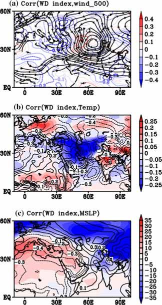
59       Page 2 of 14                                       J. Earth Syst. Sci. (2020)129 59

lifeline for millions of people in the Indian          Barros 2004). WDs propagate over different
subcontinent and contributes 70% of annual             countries such as Iran, Iraq, Afghanistan, Pakistan
rainfall over Indian region (Ashok et al. 2004).       and India and aAect the weather over these regions
IWM is limited over northern Indian region, but is     and become intense during winter. About 50% of
important in respect to Himalayan climate and          annual precipitation over Karakoram Himalaya is
hydrology (Dimri 2013b). The intensity of IWM          obtained due to the passage of WDs in winter
decreases with east and southward progression          (Barros et al. 2006). Associated extreme precipi-
(Yadav et al. 2012). Due to its contribution to mass   tating events during winter are harmful to nature
balance of glaciers, IWM studies are important in      (Dimri and Chevuturi 2014). WDs do not always
the context of global warming (Bookhagen and           have well-marked cold or warm fronts either at the
Burbank 2010). Seasonal snowfall and its frequency     surface or upper levels. This is how WDs differ
show a decreasing trend in winter (Shekhar et al.      from extratropical depressions (Mooley 1957).
2010). But some studies show increase in winter        WDs are embedded in subtropical westerly jet
precipitation over northwestern part of India dur-     (STJ) which provides upper-level divergence for
ing recent period (Dash et al. 2007; Yadav et al.      the intensiBcation of WDs (Puranik and Karekar
2010).                                                 2009). WDs are analyzed through its vertical
   Winter precipitation is mainly due to the           structure (Hunt et al. 2018b). Their analysis of
eastward-moving synoptic weather system known          vertical distribution of zonal wind of tracked WDs
as WDs (Pisharoty and Desai 1956; Rao and              indicates westerly jet which is strongest at
Srinivasan 1969; Mooley 1957; Dutta and Gupta          200 hPa. Mean jet speed of 40 m/s is noted ahead
1967; Mohanty et al. 1998). It originates from         of WD. A strong cyclonic circulation with wind
Mediterranean/Caspian Sea with frontal charac-         speed of 10 m/s is observed at upper troposphere in
teristics similar to that of extratropical storms      the vertical cross-section of meridional wind. WDs
(Dhar et al. 1984) but gradually loses its frontal     have a lifecycle of 3–4 days (Dutta and Gupta
nature due to lowering of pressure and tempera-        1967). But it may differ in accordance with the
ture gradients (Rao and Rao 1971). Moreover, it        intensity of WDs. If multiple WDs occur continu-
gets intensiBed due to incursion of moisture from      ously it may have a longer life span. WDs move
Caspian and Arabian Seas and interaction with          eastwards at a rate of 5° longitudes per day. Winter
Himalayan topography which results in increased        months record 6–7 WDs per month but its fre-
precipitation (Singh et al. 1981; Dimri and Niyogi     quency decreases in summer (Rao and Srinivasan
2013). Hunt et al. (2018a) assessed moisture           1969). Mohanty et al. (1998) reported the occur-
sources for drought, median and heavy rainfall         rence of 4–6 WDs during the winter season
events during winter season using Lagrangian           (November–March). The occurrence of WDs over a
method. Their study revealed that sources of           region does not ensure precipitation as it depends
moisture are different during each event. The          on the availability of moisture and instability
source of moisture during dry events was from          conditions during its propagation. WDs form a
Arabian peninsula. For median rainfall event, the      trough in westerlies at 500 hPa level. The position
air parcels originated in the Arabian peninsular       of trough in westerlies determines the strength and
region and Oman. For the wet case, air parcels         vertical extent of it.
having originated from Persian Gulf were associ-          Geopotential height is commonly used by the
ated with cyclonic disturbances over the Hindus-       scientiBc community to study WDs because deep
tan domain which advects northerlies and is found      trough within the extratropical cyclones exhibits
to co-occur with passing WDs observed by Hunt          distinctive signature. Heavy precipitation events
et al. (2018b). Thermo-dynamical study of WDs          over central Himalaya (CH) are associated with
highlight that additional source of moisture is        500 hPa geopotential height and this relation is
required for the precipitation related to WDs.         used by Lang and Barros (2004) to analyze WD
Convective activity is detected as the increase in     activity. An increase in precipitation is linked with
value of convective available potential energy         more troughs in westerlies which is related to
(CAPE) during the propagation of WDs (Roy and          increased variability in 500 hPa height. Cannon
Bhowmik 2005).                                         et al. (2015) studied frequency and magnitude of
   The amount of precipitation received in the         WDs using 200 hPa geopotential height anomalies
Himalayas is not linearly linked with the dynamics     and found enhancement in WDs activity leads to
associated with the intensity of WDs (Lang and         local heavy precipitation over Karakoram/western
J. Earth Syst. Sci. (2020)129 59                                                         Page 3 of 14 59

Himalaya (KH) and CH. Ridley et al. (2013)               winter period 1986/1987 to 2015/2016 is also used.
predicted future WDs activity using projections          The resolution of the NCEP/NCAR reanalysis is at
from a regional climate model. An increase in the        2.5° with 12 pressure levels from 1000 to 100 hPa.
occurrence of WDs and snowfall is observed by            The WD index is developed using NCEP/NCAR
2100. An increase in heavy precipitation events          data. In order to validate the index, Era-Interim
over western Himalaya (WH) in recent decades is          reanalysis data with spatial resolution of 0.75° pro-
linked to increased baroclinicity of the westerly        vided by European Centre for Medium-Range
winds which enhanced variability of WDs (Mad-            Weather Forecasts (ECMWF) (Dee et al. 2011) is
hura et al. 2015). They constructed a quantitative       used. The number of WDs for the study period is
index describing the activity of WDs using 500 hPa       obtained from Indian Daily Weather Reports
geopotential height.                                     (IDWR) of the India Meteorological Department
   Sometimes, these WDs in association with other        (IMD) which provides daily observations recorded
local/synoptic-scale weather systems cause severe        at 0830 hrs IST. The WDs number per season for
weather such as hailstorms leading to destruction of     each year are provided in table 1.
property and crops (De et al. 2005); avalanches
which result in collapse of snow cover in the moun-
                                                         2.2 Methods
tains (Rangachary and Bandyopadhyay 1987); fog
under stable atmospheric conditions, i.e., moisture      More than 500 cases of WDs are analyzed during the
availability along with low wind speed (Rao and          study period. Changes in pressure, temperature and
Srinivasan 1969; Syed et al. 2012), and cold waves
associated with the departure of temperature from           Table 1. Number of WDs occurred during winter sea-
normal minimum temperature (Mooley 1957). Thus              son (December, January, February – DJF) per year
in recent times with concurrent understanding, it           during 1986–2016 period
becomes imperative to understand WDs.
                                                            Year                                   No. of WDs
   The present study focuses on investigating the
percentage contribution of winter precipitation due         1987                                       23
to WDs and proposes a Western Disturbance Index             1988                                       21
                                                            1989                                       24
(WDI) using the difference of 850 and 200 hPa
                                                            1990                                       18
geopotential height. Characteristics of WDs are
                                                            1991                                       20
analyzed using this index to correspond it with the         1992                                       19
possibility of future prediction and associated             1993                                       19
dynamics.                                                   1994                                       17
                                                            1995                                       26
                                                            1996                                       25
2. Data and methods                                         1997                                       20
                                                            1998                                       19
                                                            1999                                       18
2.1 Data
                                                            2000                                       14
Precipitation data used in this study are obtained          2001                                       16
                                                            2002                                       20
from the Climate Prediction Centre (CPC) global
                                                            2003                                       21
daily uniBed gauge-based analysis of precipitation
                                                            2004                                       26
(Chen et al. 2008). The data is available at 0.5°           2005                                       21
resolution over global land areas, starting from 1979.      2006                                       21
The data comprises historical observations, satel-          2007                                       21
lites, radars and numerical model forecasts to              2008                                       23
maintain higher precision. Orographic eAects are            2009                                       19
also considered in creating precipitation data (Xie         2010                                       23
et al. 2007). National Center for Environmental             2011                                       17
Prediction/National Center for Atmospheric                  2012                                       14
Research (NCEP/NCAR) (Kalnay et al. 1996) daily             2013                                       18
mean reanalysis of surface air temperature, wind            2014                                       16
                                                            2015                                       10
and geopotential height at different levels, omega at
                                                            2016                                       13
500 hPa, and mean sea level pressure (MSLP) for the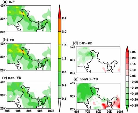
59 Page 4 of 14 J. Earth Syst. Sci. (2020)129 59
wind occur during the passage of WDs both at the receives considerable amount of precipitation
lower and upper troposphere (Dimri 2006). For this during winter as WDs interact with Himalayas
reason, we have used lower (850 hPa) and upper thus providing orographic forcings. The following
(200 hPa) tropospheric geopotential height for con- sections elaborate on the basic Belds, and there-
structing WDI. The thickness between 850 and after on WDI.
200 hPa level is proportional to mean temperature as
well as moisture of air between those levels. Empir- 3.1 Basic Belds
ical Orthogonal Function (EOF) method is used for
analyzing variability of geopotential height, zonal Precipitation climatology of WDs and non-WD
wind and meridional wind. The spatial pattern of days during winter is shown in Bgure 2. A higher
variability and its time variation is identiBed from amount of precipitation is obtained during WD
this method. Spatial patterns are known as EOFs days over Karakoram, Hindukush and Sulaiman
and time series are known as Principal Components ranges (Bgure 2b). Heavy precipitation occurs near
(PCs) (Wilks 1995; Kutzbach 1967; JolliAe 2002). hilly areas due to the complex orographic interac-
The Brst pattern explains largest part of the variance tion of WDs with high mountain ranges (Dimri and
and second pattern explains largest part of the Niyogi 2013). Though not all the WDs precipitate
remaining variance and so on. heavily, few of them produce heavy precipitation.
WDs cause heavy precipitation in WH usually in
the form of snow (Ridley et al. 2013). Winter pre-
3. Results and discussion
cipitation is the sum of WD days and non-WD days
precipitation (Bgure 2a). Non-WD days produce
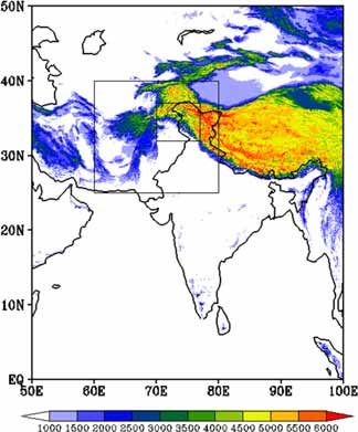
The topography of the study area is shown in
lower amount of precipitation (Bgure 2c). The
Bgure 1. Most WDs are found to be concentrated
average amount of precipitation during DJF is less
within the large box of area 25–40°N, 60°–80°E and
than that of WD days. To analyze spatial vari-
is therefore considered for the present study. A
ability, average precipitation during DJF is sub-
smaller box of area 32–37°N, 70–77°E is used to
tracted from the mean precipitation during WDs
average precipitation in the present study. WH
(Bgure 2d). Higher precipitation during WD days
than DJF is observed over Karakoram region.
Similarly, average precipitation during non WDs is
subtracted from WDs in Bgure 2(e). Higher pre-
cipitation over WH, Hindukush and Sulaiman
ranges indicates that large amount of precipitation
is obtained over this region during WD days com-
pared to non-WDs.
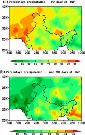
Percentage precipitation for WDs and non-WD
days is shown in Bgure 3(a and b) respectively.
WDs contribute 80% of winter precipitation over
Afghanistan, Pakistan and northern India. This
winter precipitation is mainly due to the interac-
tion of WDs with the Himalayas. In non-WD days,
*20% of winter precipitation over Afghanistan,
Pakistan and northern India is observed. WH is
characterized by heterogeneous topography with
highly nonlinear land–atmosphere interactions.
Interaction of WDs with WH determines amount
of winter precipitation obtained over the region.
Precipitation is mostly in the form of snow over
WH (Dimri 2012). The water budget over the high
mountain areas depends on the topography and
land use of the area (Fairman et al. 2011).
Figure 1. Topography (m: shade). The area of 25–40°N,
60–80°E is considered to deBne the Western Disturbance
The spatial distribution of seasonal precipitation
Index (WDI). The area of 32–37°N, 70–77°E is considered for cannot completely distinguish the behaviour of
averaging precipitation in the present study. precipitation during DJF and WD days. Therefore,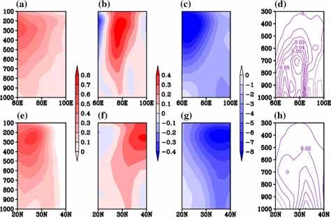
J. Earth Syst. Sci. (2020)129 59                                                            Page 5 of 14 59

Figure 2. Precipitation climatology (mm/day) in (a) December, January, February (DJF) (b) WD days of DJF (c) non-WD
days of DJF (d) DJF-WD days (e) nonWD-WD days averaged during 1986–2016 period. In Bgure (d) and (e) negative values
indicate higher precipitation during WD days compared to DJF and non-WD days.

the frequency distribution of precipitation is             that high precipitation ranges are seen during WD
plotted during DJF and WD days to better                   days.
understand the spatial variability of precipitation           In order to verify the major amount of
intensity. The entire range and frequency of pre-          precipitation during WD days due to the occur-
cipitation can be estimated in a more coherent             rence of WDs, the correlation map between
manner by this method. DJF and WD days mean                monthly precipitation and monthly WD days is
precipitation intensity along with their frequency         plotted and is shown in Bgure 5. Correlation coef-
in percentage is plotted (Bgure 4). The probability        Bcients of 0.4–0.6 are seen over the northwest part
distribution function is plotted as gamma distri-          of India and associated regions during the month of
bution curve. Gamma distribution is an excellent           December. The low correlation coefBcients are due
choice for describing precipitation parameters in          to non-homogenous in situ station data obtained in
areas with low mean and high variability in pre-           these high altitude regions. The complex orography
cipitation (Husak et al. 2007). The extended tail to       of the region is an obstacle to monitoring precipi-
the right of the distribution is advantageous in           tation. Most of the in-situ stations are situated in
representing extreme rainfall events (Ananthakr-           low altitude regions, and very few are present in
ishnan and Soman 1989). Flexibility in shape of the        mountain tops where there is a chance for heavy
gamma distribution function allows it to Bt any            precipitation (Archer and Fowler 2004). Thus
number of rainfall regimes. Each curve is identiBed        precipitation in high altitude regions is not mea-
with two parameters: shape parameter (a) and               sured. Snowfall in high altitude region is also
scale parameter (b). There is a close resemblance in       poorly measured (Rasmussen et al. 2012).
shape parameter, a between DJF and WD curve.                  Figure 6 shows an interannual variation of
Most of the precipitation is concentrated in the           precipitation during DJF, WD days of DJF and
range of 0.6–0.8 mm/day for both DJF and WD.               non-WD days of DJF during 1986–2016 period.
But the frequency of peak precipitation in the             Precipitation is area averaged over the region
intermediate range is slightly higher for DJF.             32°–37°N, 70°–77°E. Cumulative averaged precip-
Longer tail observed in the WD curve indicates             itation is more during WD days compared to
59                 Page 6 of 14                                                     J. Earth Syst. Sci. (2020)129 59

                                                                               Figure 5. Correlation between monthly precipitation and
Figure 3. Percentage precipitation in (a) WD days of DJF                       monthly WD days for (a) Dec, (b) Jan and (c) Feb during
and (b) non-WD days of DJF averaged during the 1986–2016                       the 1986–2016 period. Shown in contours are correlation
period. WD days contribute 80–90% of precipitation over                        coefBcients.
western Himalayas.

     100                                                                       precipitation is observed during DJF and WD days
         90                                                                    in 2009 and 2013. About 19 and 18 WDs occurred
         80                                         DJF-precip
                                                                               in these years, respectively. In the year 2013, non-
         70                                         WD-precip                  WD days show nil precipitation. So, precipitation
         60                                                                    during 2013 winter is mainly due to WDs. In
PDF(%)

         50                                                                    addition, in year 2014, non-WD days yield higher
         40                                                                    amount of precipitation. These anomalous cases
         30                                                                    need further investigation and study in future.
         20                                                                       Longitudinal versus vertical cross-sectional
         10                                                                    distribution of zonal wind, meridional wind and
         0                                                                     geopotential height and speciBc humidity averaged
              0   0.2 0.4 0.6 0.8    1   1.2 1.4 1.6 1.8    2    2.2 2.4 2.6   over 20–40°N latitude is shown in Bgure 7a–d. The
                                    Precipitaon(mm/day)
                                                                               maximum zonal wind is observed at mid- to upper-
Figure 4. Probability Distribution Function (PDF) for rain-                    troposphere over 60–80°E longitude with core of
fall intensities during DJF and WD days of DJF over                            maxima at 300 hPa. The higher meridional wind is
1986–2016 period.                                                              found over 70–85°E from 700–100 hPa. Negative
                                                                               values of geopotential height are also observed
non-WD days. WD days and DJF show almost                                       from mid- to upper-troposphere. Further, latitu-
similar precipitation amount except during few                                 dinal versus vertical cross-section of these variables
years. As shown in Bgure, in years 1987, 2006, and                             averaged over 60–100°E longitude is shown in
2014 higher precipitation during non-WD days is                                Bgure 7e–h, respectively. Zonal wind maxima are
received as compared to other years. Higher                                    found at 250 hPa over 20–35°N latitude,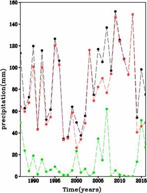
J. Earth Syst. Sci. (2020)129 59                                                                 Page 7 of 14 59

meridional wind maxima at 300 hPa over 30–40°N                 at 300 hPa over 25–40°N latitude. Positive
latitude and negative geopotential height minima               (negative) values of zonal wind denote westerly
                                                               (easterly) wind (wind coming from west (east)).
                                                               Similarly, positive (negative) value of meridional
                                                               wind indicates southerly (northerly). Negative
                                                               values of geopotential height indicate low-pressure
                                                               area or trough which mainly occurs during pre-
                                                               cipitating WDs (Dimri 2006). A maximum geopo-
                                                               tential anomaly is found at 200 hPa.
                                                               Comparatively fewer values are found at 500 hPa
                                                               level. But 500 hPa geopotential height is the
                                                               commonly used variable to represent atmospheric
                                                               circulation and is also used to predict other mete-
                                                               orological variables (Zheng and Frederiksen 2007).
                                                               A trough is associated with cloudy conditions and
                                                               precipitation or it can bring in cold air mass. These
                                                               Bgures indicate that southwesterly wind and
                                                               trough forms over northwest part of India during
                                                               the passage of WDs. The southwesterly wind
                                                               brings moisture from Arabian Sea which leads to
                                                               widespread precipitation over WH. Seasonal anti-
                                                               cyclone formed over central India at 0.9 km above
                                                               sea level controls this moisture intake (Rangachary
                                                               and Bandyopadhyay 1987).
                                                                  SpeciBc humidity is used to describe the mois-
                                                               ture Beld in the present study. It is the ratio of the
Figure 6. Time-series of cumulative seasonal precipitation
(mm) during DJF (black line), WD days of DJF (red line),
                                                               mass of water vapour to total mass of air. Wet
non-WD days of DJF (green line) averaged over the region       anomaly is found in the lower troposphere. As we
(32–37°N,70–77°E) during 1986–2016 period.                     go upwards moisture content decreases and dry

Figure 7. Longitude-pressure vertical cross-section averaged over 20°–40°N latitude for (a) Zonal wind(m/s) (b) Meridional
wind (m/s) (c) Geopotential height (m) (d) SpeciBc humidity (g/kg). Latitude-pressure vertical cross-section averaged over
60°–100°E longitude for (e) Zonal (m/s) (f) Meridional (m/s) and (g) Geopotential height (m) (h) SpeciBc humidity (g/kg) of
(WD minus DJF) days during 1986–2016 period. Positive zonal and Meridional wind denotes south westerly wind and negative
Geopotential height indicates low-pressure area or trough.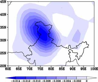
59       Page 8 of 14                                          J. Earth Syst. Sci. (2020)129 59

anomaly is seen in the mid-upper troposphere              distribution of westerlies is seen at mid-tropo-
(Bgure 7d). Changes in speciBc humidity are more          spheric levels with lesser magnitude (Bgure 9b). At
observed in the longitude–pressure vertical               lower troposphere westerlies are not seen
cross-section.                                            (Bgure 9c). The upper-level cyclonic situation
   Omega at 500 hPa is used to analyze vertical           which developed due to strong westerlies is able to
motion (ascending or descending motion) of                ascend the moisture rapidly resulting in cloud for-
air/mass and is shown in Bgure 8. Negative values         mation and heavy precipitation over the region.
of omega indicate ascending motion of air and                The difference between geopotential height
positive values imply descending of air. The              anomalies at 850 and 200 hPa is calculated over the
upward motion of air leads to increase in relative        region 25–40°N, 60–80°E and is shown in
humidity through large depth of atmosphere which          Bgure 11(a). This region is selected as maximum
further results in clouds and precipitation. On the       dynamics associated with WDs and associated
availability of moisture in vertical air column due       precipitation occurs over here. Dimri and Chevu-
to incursion from Arabian Sea, possibility of pre-        turi (2014) established that vertical distribution of
cipitation forming mechanism will be expedited.           geopotential height anomaly shows a northwestern
Negative values of omega i.e. strong ascend is seen       tilt in vertical axis of the WDs. During early stage
ahead of WDs over WH during the passage of WDs            of WDs, the low-pressure region shows northwest-
which is found to be maximum at 450 hPa followed          ern tilt which becomes northeasterly with subse-
by a descending (Hunt et al. 2018b) which leads to        quent propagation of WDs. Thus vertical
strong upward movement of air, as a result                difference between 850 and 200 hPa is proportional
orographic lifting of moisture occurs.                    to volume over the speciBed region which further
   Circulation and geopotential height at 200, 500        depends on mean temperature of air between these
and 850 hPa are illustrated in Bgure 9(a–c)               levels. The thickness of air is a measure of coldness
respectively. Geopotential height is plotted in           or warmness of air. Geopotential height anomaly at
contours. A strong band of negative geopotential is       upper level is low during winter compared to lower
seen between 25 and 50°N latitude centered at             level. Geopotential height anomaly at upper tro-
200 hPa (Bgure 9a) along with southwesterly winds         posphere is subtracted from lower troposphere
traveling from western part of continent towards          results in large positive value during winter season.
northwest part of India and WH region. The strong         As shown in Bgure 11(a) values start increasing
westerlies are capable of bringing moisture from          from November onwards and attain maximum
Arabian Sea which thus will sustain WDs and               value in January and February and after that it
leading to intensiBcation of IWM. A similar               starts decreases.

                                                          3.2 Western Disturbance Index

                                                          Winter WDs have asymmetric upper air trough
                                                          which has similar characteristics of Bjerknes
                                                          cyclones of paciBc and Atlantic (Pisharoty and
                                                          Desai 1956). The energy discharge and develop-
                                                          ment of WDs can be explained by baroclinic
                                                          instability (Rao and Rao 1971). This instability
                                                          arises due to the meridional temperature gradient.
                                                          WDs which result in heavy precipitation, has deep
                                                          upper-level trough which is located westward and
                                                          shows vertical tilting (Cannon et al. 2015). Model
                                                          analysis indicates a northwestern tilt in geopoten-
                                                          tial anomaly during the early growth stage of WDs
                                                          (Dimri and Chevuturi 2014). Cyclones growing by
                                                          baroclinic processes are expected to tilt upshear.
                                                          This westward tilt is important because potential
Figure 8. Omega (Pa/s*10-3) at 500 hPa of WD averaged
during the 1986–2016 period. Negative omega values show   energy is provided to the disturbance by mean Cow
upward motion.                                            through this (Holton and Hakim 2012). The
J. Earth Syst. Sci. (2020)129 59 Page 9 of 14 59
Bgure 9. Wind (m/s: vector) and geopotential height (m: contour) for (WD minus DJF) days at (a) 200 hPa, (b)500 hPa and
(c) 850 hPa averaged during 1986–2016 period. Stronger south westerlies and trough occurs at middle and upper troposphere.
Figure 10. Potential vorticity (10-8 K kg-1 m2s-1) for (WD minus DJF) days at (a) 200 hPa, (b) 250 hPa (c) 300 hPa averaged
during 1986–2016 period.
(b) 3 30
2.5
2 25
1.5
20
1
No of WDs
0.5
WDindex
(a) 15
400 0
300
-0.5
200 10
HGT850-HGT200
100
-1
0
-100 -1.5 5
-200
-300 -2
-400
-500 -2.5 0
MAR
MAY
AUG
NOV
OCT
DEC
APR
JAN
JUN
FEB
JUL
SEP
1987 1992 1997 2002 2007 2012
Years
Months
No.of WDs WDindex-NCEP
Figure 11. (a) Time-series of difference between geopotential height (m) anomaly at 850 and 200 hPa (850 minus 200) averaged
over region 25°–40°N, 60°–80°E and (b) Time series of WDI and number of WDs. WDI is plotted as lines. The bar graph shows
the number of WDs.
baroclinicity of basic state interplay with moist baroclinicity to perturbation development (Cohen
convection leads to disturbance growth. Potential and Boos 2016).
vorticity anomalies inCuence the mean vertical Potential vorticity (PV) is analyzed to establish
shear to transfer energy from the mean the evolution of WDs in a baroclinic background59 Page 10 of 14 J. Earth Syst. Sci. (2020)129 59
Many WD studies focus on the variability of
geopotential height since it has trough in upper
level. Lang and Barros (2004) noted an increase in
precipitation related to WDs over CH when there
is increased variability of 500 hPa geopotential
height. Cannon et al. (2016) developed a wave
tracking methodology to track WDs using 500 hPa
geopotential height anomalies since WDs can be
differentiated with its depression in 500 hPa
geopotential height.
On account of these factors, difference between
850 and 200 hPa geopotential height anomaly
(refer to Supplementary Bgure S1) is considered to
formulate and propose WDI. The seasonal mean
value of geopotential height anomaly (averaged
over the area of 25°N 60°E to 40°N 80°E) at 850
and 200 hPa is calculated. Further, the value at
850 hPa is subtracted from 200 hPa. Then it is
divided by standard deviation to construct stan-
dardized WDI. The index is calculated using
NCEP data and further veriBed by using ERA-
Interim reanalysis data. WDI calculated using
NCEP and ERA shows almost similar values
(shown in Supplementary Bgure S2), so for our
convenience we are using NCEP WDI data in fur-
ther analysis. As WDI increases temperature
decreases and vice versa. WDI along with trend
line is plotted against number of WDs during
winter for each year and is illustrated in
Bgure 11(b). WDI increases with number of WDs
in almost all the years except in few years. This is
because WDI may depend upon intensity of WDs.
The correlation coefBcient between WDI and
number of WDs is found to be 0.1788. The poor
correlation between the two may be due to the fact
Figure 12. Spatial pattern of correlation between WDI and
that not all WDs are strong enough to create large
(a) 500 hPa wind (streamlines in m/s), blue contour line
corresponds to negative correlation and red contour line dip in upper troposphere geopotential height which
corresponds to positive correlation, (b) 2m temperature leads to more precipitation over the region. Only
(shaded in degree C), (c) Mean Sea Level Pressure (MSLP, 5% of WDs lead to heavy precipitation (Hunt et al.
shaded in meter) for WD minus DJF days averaged during 2018b). As the intensity of WDs increases, the
1986–2016. The positive correlation is shown in black solid trough deepens in geopotential height at upper
contours and negative correlation is shown in broken line
contours.
levels. Madhura et al. (2015) calculated WD index
based on EOF analysis of daily geopotential height
(Bgure 10) state. The structure of PV in the upper anomaly and standard deviation of PC1. A positive
atmosphere is similar to that of baroclinic waves trend in WD index indicates enhanced variability
(Hunt et al. 2018b). The high value of PV is in WDs and thus heavy precipitation over WH
observed in cyclogenesis conditions. Low geopo- during recent periods. WDI in a way provides a
tential height observed over the region (Bgure 9a) comprehensive view of the vertical structure asso-
corresponds to large PV values (Bgure 10a). ciated with the WDs. However, there are few
WDs are considered as eastward moving anomalous seasons when they are not in coherence
extratropical cyclones (Barlow et al. 2005). WDs to each other and thus needs further investigation.
are characterized by deep upper-level trough and In order to validate the WDI, correlations
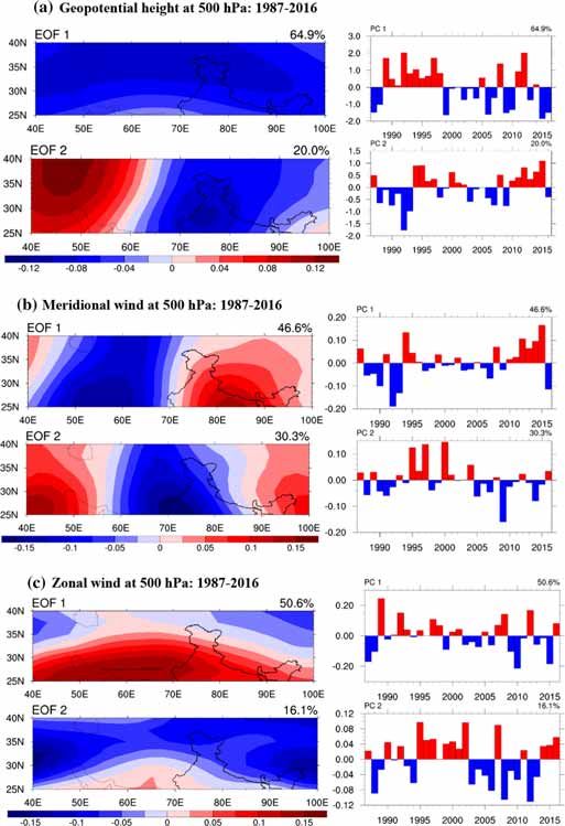
existence of surface low (Singh and Kumar 1977). between WDI with variables, viz., 500 hPa wind, 2J. Earth Syst. Sci. (2020)129 59 Page 11 of 14 59 Figure 13. EOF/PC analysis of daily (a) geopotential height, (b) meridional wind and (c) zonal wind at 500 hPa for WD days of DJF season based on NCEP data over the domain 25–40°N,40–100°E during 1987–2016 period. The spatial pattern of the Brst mode is EOF1 and the spatial pattern of the second mode is EOF2. The Brst and second modes explain 64.9 and 20.0%, 46.6 and 30.3%, 50.6 and 16.1% of the total variance for (a), (b) and (c) respectively. m air temperature and MSLP during WD minus WDI over the Hindukush and Sulaiman range DJF days averaged during 1986–2016 are calcu- (Bgure 12a). That explains about the sustaining of lated. 500 hPa wind during the WD minus DJF WD over this area. A negative correlation is noted days averaged during 1986–2016 shows cyclonic over rest of the region. This suggests a divergence circulation over the Himalayas and adjacent of mass from the rest of the region. During the regions. 500 hPa wind is positively correlated with period, warmer temperature over central India and
59       Page 12 of 14                                       J. Earth Syst. Sci. (2020)129 59

colder temperature over regions northwest of            above analysis EOF1 can be considered as the
Indian subcontinent is observed. This temperature       spatial pattern of geopotential height and PC1 is
is negatively correlated with WDI over northern         the interannual variability of amplitude of EOF1
India, central Asia, Arabian Sea, Indian Ocean and      during the occurrence of WDs over the speciBed
Bay of Bengal and positively correlated over the        domain. EOF1 pattern of meridional wind explains
regions west of central Asia and central India. It is   46.6% variance and EOF2 30.3% of total variance.
important to note that, in northern part of India       While PC1 and PC2 with loading vector 0.20 to
warmer temperature is found which is negatively         –0.20 are seen. The negative component of merid-
correlated with WDI (Bgure 12b). This suggests          ional wind delineates northerly and positive com-
cold air incursion towards India during the propa-      ponent southerly wind (Bgure 13b). Strong
gation of WDs. After the passage of WDs, cold air       northerly wind is seen over Pakistan and south-
from northern latitude moves towards India which        erly wind over Indian region. EOF1 pattern of
leads to cold wave conditions (De et al. 2005).         zonal wind shows strong westerly jet over
MSLP patterns indicate higher pressure over west        Pakistan and India with 50.6% variance and
of Indian subcontinent and lower pressure over          EOF2 explains 16.1% of total variance
India, northern latitudes and east of Indian sub-       (Bgure 13c). However, PC1 shows temporal vari-
continent (Bgure 12c). Intense low pressure over        ability in range of loading vector 0.25 to –0.25.
Tibetan and central to northern India pulls the         PC2 shows 0.12 to –0.12. Meridional variability of
mass from Mediterranean Sea, which is an intense        jet can be seen during the propagation of WDs.
high-pressure region. That is why Tibetan and           Thus, EOF1 pattern of geopotential height; zonal
central to northern India is positively correlated      wind and meridional wind indicate movement of
with coefBcient values 0.4–0.2. However, Mediter-       WDs over the domain.
ranean Sea, the west-south Asian region and the
northeast Africa region are negatively correlated
with coefBcient values –0.4 to –0.2. During the         4. Conclusions
passage of WDs, low-pressure area is seen over
northern part of India and Pakistan. The lows are       The objective of this research is to investigate the
associated with ascending/converging air masses         climatology of WDs and the construction of a
which leads to showers over the region. MSLP            WDI. More than 500 WD cases from the IDWR are
shows positive correlation with WDI over this           used to analyze the climatology of WDs. Precipi-
region. The newly constructed WDI explains some         tation climatology is calculated for entire winter
of the variances of 500 hPa wind, 2 m air temper-       season, during the occurrence of WDs and non-WD
ature and MSLP in the course of advancement of          days and concluded that WDs produce significant
WDs over Indian region.                                 amount of precipitation over WH and northern
   EOF analysis is applied to 500 hPa daily             part of India during winter. WDs contribute to
geopotential height over the domain 25–40°N,            more than 80% of precipitation over northwest
40–100°E during the 1987–2016 period for WD             part of India and Pakistan during winter season.
days of DJF. The spatial patterns of Brst two EOFs      Vertical distribution of geopotential height and
(EOF1 and EOF2) and its time series known as            winds indicate a trough and southwesterly direc-
Principal Components (PC1 and PC2) are shown            tion respectively during WDs which shows mois-
in Bgure 13. It can be seen that EOF1 pattern           ture incursion from Arabian Sea. Negative omega
shows negative all over the domain (Bgure 13a).         values at 500 hPa indicate convergence and
More negative values are found over 30–35°N lat-        increase in humidity which results in precipitation.
itude. The EOF1 pattern explains 64.9% variance.        A new WDI for IWM is proposed using difference
PC1 shows change in amplitude of EOF1 with              of 850 and 200 hPa geopotential height and is
time. The intensity and frequency of negative           validated using different variables such as 500 hPa
amplitude are increasing in recent years. It is noted   wind, air temperature and MSLP. Wind at 500 hPa
that EOF2 pattern shows negative geopotential           is positively correlated with WDI over Hindukush
height over WH and Pakistan and positive is seen        and Sulaiman range. Air temperature and WDI
further westward (Bgure 13a). Strong positive           show a negative correlation over north India.
geopotential height is seen over 35°N, 45°E. EOF2       Negative MSLP is positively correlated with WDI
pattern shows northwest–southeast orientation.          over north India. The Brst pattern of EOF of
EOF2 pattern explains 20% variance. From the            geopotential height, zonal wind and meridional
J. Earth Syst. Sci. (2020)129 59                                                                   Page 13 of 14 59

wind shows the propagation of WDs during winter                     activity aAecting the Himalaya; Clim. Dyn. 44(1–2)
season over the domain.                                             441–455, https://doi.org/10.1007/s00382-014-2248-8.
                                                                  Chen M, Shi W, Xie P, Silva V B, Kousky V E, Wayne Higgins
                                                                    R and Janowiak J E 2008 Assessing objective techniques for
                                                                    gauge-based analyses of global daily precipitation; J.
Acknowledgements                                                    Geophys.       Res.       113,     https://doi.org/10.1029/
                                                                    2007JD009132.
The authors acknowledge National Center for                       Cohen N Y and Boos W R 2016 Perspectives on moist
Environmental Prediction/National Centre for                        baroclinic instability: Implications for the growth of mon-
Atmospheric Research for providing dataset. The                     soon depressions; J. Atmos. Sci. 73(4) 1767–1788, https://
                                                                    doi.org/10.1175/JAS-D-15-0254.1.
authors are also thankful to CPC for providing                    Dash S K, Jenamani R K, Kalsi S R and Panda S K 2007 Some
precipitation datasets. The work of Midhuna T M                     evidence of climate change in twentieth-century India;
was supported by Junior Research Fellowship                         Clim. Change 85 299–321, https://doi.org/10.1007/s10584-
granted by Department of Science and Technology.                    007-9305-9.
Special thanks to Madhavi Jain for improving the                  De U S, Dube R K and Rao G P 2005 Extreme weather events
                                                                    over India in the last 100 years; J. Ind. Geophys. Union
English of the manuscript.
                                                                    9(3) 173–187.
                                                                  Dee D P, Uppala S M and Simmons A J et al. 2011 The ERA-
                                                                    Interim reanalysis: ConBguration and performance of the
                                                                    data assimilation system; Quart. J. Roy. Meteorol. Soc. 137
References                                                          553–597.
                                                                  Dhar O N, Kulkarni A K and Sangam R B 1984 Some aspects
Ananthakrishnan R and Soman M K 1989 Statistical distri-            of winter and monsoon rainfall distribution over the
  bution of daily rainfall and its association with the             Garhwal–Kumaun Himalayas – a brief appraisal; Him.
  coefBcient of variation of rainfall series; Int. J. Climatol.     Res. Dev. 2(2) 10–19.
  9(5) 485–500.                                                   Dimri A P 2012 Wintertime land surface characteristics in
Archer D R and Fowler H J 2004 Spatial and temporal                 climatic simulations over the western Himalayas; J. Earth
  variations in precipitation in the Upper Indus Basin, global      Syst. Sci. 121(2) 329–344, https://doi.org/10.1007/s12040-
  teleconnections and hydrological implications; Hydrol.            012-0166-x.
  Earth Syst. Sci. 8 47–61, https://doi.org/10.5194/hess-8-       Dimri A P 2006 Surface and upper air Belds during extreme
  47-2004.                                                          winter precipitation over the western Himalayas; Pure
Ashok K, Guan Z, Saji N H and Yamagata T 2004 Individual            Appl. Geophys. 163(8) 1679–1698, https://doi.org/10.
  and combined inCuences of ENSO and the Indian Ocean               1007/s00024-006-0092-4.
  Dipole on the Indian summer monsoon; J. Climate 17(16)          Dimri A P 2013a Interannual variability of Indian winter
  3141–3155, https://doi.org/10.1175/1520-0442(2004)017%            monsoon over the Western Himalayas; Global Planet.
  3c3141:IACIOE%3e2.0.CO;2.                                         Change 106 39–50, https://doi.org/10.1016/j.gloplacha.
Barlow M, Wheeler M, Lyon B and Cullen H 2005 Modulation            2013.03.002.
  of daily precipitation over southwest Asia by the Mad-          Dimri A P 2013b Intraseasonal oscillation associated with the
  den–Julian Oscillation; Mon. Wea. Rev. 133(12)                    Indian winter monsoon; J. Geophys. Res: Atmos. 118(3)
  3579–3594, https://doi.org/10.1175/MWR3026.1.                     1189–1198, https://doi.org/10.1002/jgrd.50144.
Barros A P, Chiao S, Lang T J, Burbank D and Putkonen J           Dimri A P and Chevuturi A 2014 Model sensitivity analysis
  2006 From weather to climate – Seasonal and interannual           study for western disturbances over the Himalayas; Mete-
  variability of storms and implications for erosion processes      orol. Atmos. Phys. 123(3–4) 155–180, https://doi.org/10.
  in the Himalaya; In: Tectonics, Climate, and Landscape            1007/s00703-013-0302-4.
  Evolution; Geol. Soc. Am. Spec. Paper 398 17–38.                Dimri A P and Niyogi D 2013 Regional climate model
Benn D I and Owen L A 1998 The role of the Indian summer            application at subgrid scale on Indian winter monsoon over
  monsoon and the mid-latitude westerlies in Himalayan              the western Himalayas; Int. J. Climatol. 33(9) 2185–2205,
  glaciation: Review and speculative discussion; J. Geol. Soc.      https://doi.org/10.1002/joc.3584.
  155 353–363, https://doi.org/10.1144/gsjgs.155.2.0353.          Dimri A P, Yasunari T and Kotlia B S et al. 2016 Indian
Bookhagen B and Burbank D W 2010 Toward a complete                  winter monsoon: Present and past; Earth-Sci. Rev. 163
  Himalayan hydrological budget: Spatiotemporal distribu-           297–322, https://doi.org/10.1016/j.earscirev.2016.10.008.
  tion of snowmelt and rainfall and their impact on river         Dutta R K and Gupta M G 1967 Synoptic study of the
  discharge; J. Geophys. Res. 115(F3), https://doi.org/10.          formation and movement of western depression; Indian J.
  1029/2009JF001426.                                                Meteorol. Geophys. 18(1) 45.
Cannon F, Carvalho L M, Jones C and Norris J 2016 Winter          Fairman J G, Nair U S, Christopher S A and M€      olg T 2011
  westerly disturbance dynamics and precipitation in the            Land use change impacts on regional climate over Kili-
  western Himalaya and Karakoram: A wave-tracking                   manjaro; J. Geophys. Res. 116(D3), https://doi.org/10.
  approach; Theor. Appl. Climatol. 125(1–2) 27–44,                  1029/2010jd014712.
  https://doi.org/10.1007/s00704-015-1489-8.                      Goswami B N 1994 Dynamical predictability of seasonal
Cannon F, Carvalho L M V, Jones C and Bookhagen B 2015              monsoon rainfall: Problems and prospects; Proc. Indian
  Multi-annual variations in winter westerly disturbance            Nat. Sci. Acad. Part A 60 101–120.
59 Page 14 of 14 J. Earth Syst. Sci. (2020)129 59 Holton J R and Hakim G J 2012 An introduction to dynamic avalanching in Western Himalaya; Int. Assoc. Hydrol. Sci. meteorology; Academic Press. Publ. 162 311–316. Hunt K M R, Turner A G and Shaffrey L C 2018a Extreme Rao V B and Rao S T 1971 A theoretical and synoptic study of daily rainfall in Pakistan and North India: Scale interac- western disturbances; Pure Appl. Geophys. 90(1) 193–208, tions, mechanisms, and precursors; Mon. Wea. Rev. 146(4) https://doi.org/10.1007/BF00875523. 1005–1022, https://doi.org/10.1175/MWR-D-17-0258.1. Rao Y P and Srinivasan V 1969 Discussion of typical synoptic Hunt K M R, Turner A G and Shaffrey L C 2018b The weather situation: winter western disturbances and their evolution, seasonality and impacts of western disturbances; associated features; Indian Meteorological Department Quart. J. Roy. Meteorol. Soc. 144(710) 278–290, https:// Forecast, Part III. doi.org/10.1002/qj.3200. Rees H G and Collins D N 2006 Regional differences in Husak G J, Michaelsen J and Funk C 2007 Use of the gamma response of Cow in glacier-fed Himalayan rivers to climatic distribution to represent monthly rainfall in Africa for drought warming; Hydrol. Process. 20(10) 2157–2169, https://doi. monitoring applications; Int. J. Climatol. 27(7) 935–944. org/10.1002/hyp.6209. Immerzeel W W, Beek L P H van and Bierkens M F P 2010 Climate Ridley J, Wiltshire A and Mathison C 2013 More frequent change will aAect the Asian Water Towers; Science 328(5984) occurrence of westerly disturbances in Karakoram up to 1382–1385, https://doi.org/10.1126/science.1183188. 2100; Sci. Total Environ. 468 S31–S35, https://doi.org/10. JolliAe I T 2002 Principal Component Analysis; 2nd edn, 1016/j.scitotenv.2013.03.074. Springer-Verlag, Berlin, Germany. Roy S S and Bhowmik S R 2005 Analysis of thermodynamics Kalnay E, Kanamitsu M and Kistler R et al. 1996 The NCEP/ of the atmosphere over northwest India during the passage NCAR 40-year reanalysis project; Bull. Am. Meteorol. Soc. of a western disturbance as revealed by model analysis Beld; 77(3) 437–471, https://doi.org/10.1175/1520- Curr. Sci. 88 947–951. 0477(1996)077%3c0437:TNYRP%3e2.0.CO;2. Shekhar M S, Chand H and Kumar S et al. 2010 Climate- Krishnamurti T N and Bhalme H N 1976 Oscillations of a change studies in the western Himalaya; Ann. Glaciol. monsoon system. Part I. Observational aspects; J. Atmos. 51(54) 105–112, https://doi.org/10.3189/1727564107913 Sci. 33(10) 1937–1954, https://doi.org/10.1175/1520- 86508. 0469(1976)033\1937:OOAMSP[2.0.CO;2. Singh M S and Kumar S 1977 Study of western disturbances; Kutzbach J E 1967 Empirical eigenvectors of sea-level Indian J. Meteorol. Hydrol. Geophys. 28(2) 233–242. pressure, surface temperature and precipitation complexes Singh M S, Rao A and Gupta S C 1981 Development and over North America; J. Appl. Meteorol. 6(5) 791–802, movement of a mid tropospheric cyclone in the westerlies https://doi.org/10.1175/1520-0450(1967)006%3c0791:EEO over India; Mausam 32(1) 45–50. SLP%3e2.0.CO;2. Syed F S, K€ ornich H and Tjernstr€ om M 2012 On the fog Lang T J and Barros A P 2004 Winter storms in the Central variability over south Asia; Clim. Dyn. 39(12) 2993–3005, Himalayas; J. Meteorol. Soc. Japan 82(3) 829–844, https://doi.org/10.1007/s00382-012-1414-0. https://doi.org/10.2151/jmsj.2004.829. Webster P J 1983 Mechanisms of monsoon low-frequency Madhura R K, Krishnan R and Revadekar J V et al. 2015 variability: Surface hydrological eAects; J. Atmos. Sci. Changes in western disturbances over the Western Hima- 40(9) 2110–2124, https://doi.org/10.1175/1520- layas in a warming environment; Clim. Dyn. 44(3–4) 0469(1983)040%3c2110:MOMLFV%3e2.0.CO;2. 1157–1168, http://dx.doi.org/10.1007/s00382-014-2192-7. Wilks D S 1995 Statistical Methods in Atmospheric Sciences; Mohanty U C, Madan O P, Rao P L S and Raju P V S 1998 Academic Press, San Diego. Meteorological Belds associated with western disturbances Xie P, Chen M and Yang S et al. 2007 A gauge-based analysis in relation to glacier basins of western Himalayas during of daily precipitation over east Asia; J. Hydrometeorol. winter season; Centre for Atmospheric Science, Indian 8(3) 607–626, https://doi.org/10.1175/JHM583.1. Institute of Technology, New Delhi, Technical Report. Yadav R K, Kumar K R and Rajeevan M 2012 Characteristic Mooley D A 1957 The role of western disturbances in the features of winter precipitation and its variability over production of weather over India during different seasons; northwest India; J. Earth Syst. Sci. 121(3) 611–623, Indian J. Meteor. Geophys. 8 253–260. https://doi.org/10.1007/s12040-012-0184-8. Pisharoty P R and Desai B N 1956 Western disturbances and Yadav R K, Ramu D A and Dimri A P 2013 On the relationship Indian weather; Indian J. Meteorol. Geophys. 7 333–338. between ENSO patterns and winter precipitation over north Puranik D M and Karekar R N 2009 Western disturbances and central India; Global Planet. Change 107 50–58, https:// seen with AMSU-B and infrared sensors; J. Earth Syst. Sci. doi.org/10.1016/j.gloplacha.2013.04.006. 118(1) 27–39, https://doi.org/10.1007/s12040-009-0003-z. Yadav R K, Yoo J H, Kucharski F and Abid M A 2010 Why Is Rasmussen R, Baker B, Kochendorfer J, Meyers T, Landolt S, ENSO inCuencing northwest India winter precipitation in Fischer A P and Smith C 2012 How well are we measuring recent decades? J. Climate 23(8) 1979–1993, https://doi. snow: The NOAA/FAA/NCAR winter precipitation test org/10.1175/2009JCLI3202.1. bed; Bull. Am. Meteor. Soc. 93(6) 811–829. Zheng X and Frederiksen C S 2007 Statistical prediction of Rangachary N and Bandyopadhyay B K 1987 An analysis of seasonal mean southern hemisphere 500-hPa geopotential the synoptic weather pattern associated with extensive heights; J. Climate 20(12) 2791–2809. Corresponding editor: N V CHALAPATHI RAO
You can also read