A scalable spectral Stokes solver for simulation of time-periodic flows in complex geometries
←
→
Page content transcription
If your browser does not render page correctly, please read the page content below
A scalable spectral Stokes solver for simulation of time-periodic flows in
                                                                         complex geometries

                                                                               Chenwei Menga , Anirban Bhattacharjeea , Mahdi Esmailya
                                                              a Sibley   School of Mechanical and Aerospace Engineering, Cornell University, Ithaca, NY 14850, USA
arXiv:2009.06725v2 [cs.CE] 2 Jul 2021

                                        Abstract
                                        Simulation of unsteady creeping flow in complex geometries has traditionally required the use of a time-stepping
                                        procedure, which is typically costly and unscalable. To reduce the cost and allow for computations at much larger
                                        scales, we propose an alternative approach that is formulated based on the unsteady Stokes equation expressed in the
                                        spectral domain. This transformation results in a boundary value problem with an imaginary source term proportional
                                        to the computed mode that is discretized and solved in a complex-valued finite element solver using Bubnov-Galerkin
                                        formulation. This transformed spatio-spectral formulation presents several advantages over the traditional spatio-
                                        temporal techniques. Firstly, for cases with boundary conditions varying smoothly in time, it provides a significant
                                        saving in computational cost as it can resolve time-variation of the solution using a few modes rather than thousands
                                        of time steps. Secondly, in contrast to the traditional time integration scheme with a finite order of accuracy, this
                                        method exhibits a super convergence behavior versus the number of computed modes. Thirdly, in contrast to the
                                        stabilized finite element methods for fluid, no stabilization term is employed in our formulation, producing a solution
                                        that is consistent and more accurate. Fourthly, the proposed approach is embarrassingly parallelizable owing to the
                                        independence of the solution modes, thus enabling scalable calculations at a much larger number of processors. The
                                        comparison of the proposed technique against a standard stabilized finite element solver is performed using two- and
                                        three-dimensional canonical and complex geometries. The results show that the proposed method can produce more
                                        accurate results at 1% to 11% of the cost of the standard technique for the studied cases.

                                        1. Introduction

                                             Fast and cost-effective simulation of flow in complex geometries is highly desirable, at least for two sets of applica-
                                        tions. The first is the time-critical problems where the results must be obtained in a given time window, thus imposing
                                        an upper bound on the time-to-solution. The second are those with a bound on the computational cost, where the
                                        number of CPU-hours spent on the simulation must be limited. While these two restrictions on time and cost are
                                        identical for sequential simulations, they may well diverge for parallel implementations depending on the scalability
                                        of the application.
                                             A prominent area where all the above conditions and restrictions apply is cardiovascular modeling. The flow
                                        is unsteady and time-periodic, the geometry is often complex, the cost must remain low, and the available time for
                                        simulation is often limited. A specific example within this realm is patients with congenital heart disease who must
                                        undergo an operation right after birth [1]. Utilizing cardiovascular modeling as a part of patient-specific surgical
                                        planning will require the simulation to be completed between diagnosis (birth) and the time of operation (a few days
                                        after birth at most) [2]. Moreover, performing shape optimization to improve surgical anatomy relies on having a highly
                                        efficient computational framework since a formal optimization study typically requires tens to hundreds of simulations
                                        [3]. A similar constraint exists on the efficiency of the underlying computational method if such computations were to
                                        be performed outside of the academic setting and at an industrial scale, where access to high-performance computing
                                        resources for a large number of patients remains limited due to the cost considerations [4].
                                             While there exists a broad range of numerical methods for simulating flow in complex geometries, here we consider
                                        stabilized finite element techniques to establish the relative accuracy and cost-efficiency of our method since these
                                        methods are widely adopted for cardiovascular blood flow simulation [5] and closest to the method proposed in this
                                        study. Within the realm of stabilized finite element methods (FEM), we particularly focus on the residual-based

                                        Preprint submitted to Elsevier                                                                                               July 6, 2021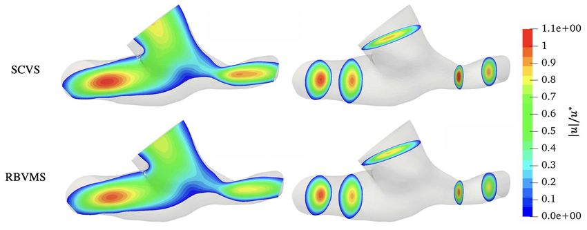
variational multiscale method (RBVMS), which is constructed on top of streamwise upwind Petrov-Galerkin (SUPG)
technique [6, 7, 8].
    As is the case with the majority of the time-dependent partial differential equations solvers, the application of
the RBVMS technique to a time-periodic problem (e.g., blood flow in the circulatory system) requires discretization
of the underlying governing equations in time. Thus, the cost of these methods is inherently dependent on the time
step size, increasing as time step size decreases. While the maximum allowable time step size is limited by the
stability considerations for explicit time integration schemes, it is often more relaxed for implicit schemes, where it
is determined solely based on the desired accuracy [9, 10]. The larger time step size for implicit schemes does not
necessarily imply their lower cost, as the fewer time steps can be offset by the larger number of Newton-Raphson
iteration per time step. Furthermore, the high cost associated with the time integration is exacerbated by the transient
nature of the solution that requires simulation of many cycles to achieve cycle-to-cycle convergence. In addition to
these setbacks, one well-known issue associated with the RBVMS formulation is its lack of consistency with regard to
time step size that, for instance, leads to the time step size dependency of the final solution obtained from a steady-state
problem.
    A remedy for the aforementioned issue is to transfer the temporal problem to a frequency domain using Fourier
transformation and subsequently solve the transformed boundary value problem mode-by-mode. Since the resulting
spectral method bypasses the time integration, its accuracy and stability are not affected by the time integration scheme.
We should note that the number of modes that must be incorporated into such calculation, at least in theory, must be
equal to the number of time steps for all time scales in the problem to be captured. However, for cardiovascular flows,
the majority of those modes can be neglected with minimal error, as we will show later in this article. In practice, a few
modes (less than ten) suffices for sufficiently smooth and time-periodic boundary conditions, thus offering a significant
reduction in overall cost in comparison to a traditional solver that requires thousands of time steps for simulation of a
single cardiac cycle [11]. On top of this saving, the spectral technique can save on the computation required for cycle-
to-cycle convergence as it is based on a boundary value problem that does not include a transient solution. Additionally,
for the linear Stokes equation that is the focus of this study, all the solution modes are orthogonal and independent,
which present two major advantages. Firstly, capturing a new mode in the solution (either due to a modification in the
boundary condition or stricter tolerance on the solution) can be done by solving one additional boundary value problem
as there is no need to recompute previous modes. The minimal cost can be contrasted against the costly alternative
of a traditional time integration scheme in which the entire computation must be repeated with a new time step size if
higher accuracy is desired. Secondly, the spectral technique can be implemented as an embarrassingly parallelizable
scheme with each group of processors computing the solution associated with only one of the many modes. Therefore,
by formulating the original temporal problem as a set of orthogonal boundary value problems, one can significantly
reduce the total computational cost and, at the same time, scale computations to a much larger number of processors.
    The enumerated advantages of formulating a problem in the spectral domain have attracted researchers to investi-
gate such schemes in the past. Perhaps the most relevant scheme to the present study that has come out of such efforts
is the development of the Time Spectral Method, which has been primarily employed by the aerospace community
for simulation of compressible flows over bluff bodies, such as blades in a compressor rotor and a pitching airfoil
[12, 13, 14, 15]. In this paper, we propose a new spatio-spectral technique named Complex-valued Stokes Solver
(SCVS) that can be differentiated from the Time Spectral Method in a number of ways. First and foremost, the afore-
mentioned Time Spectral Methods are formulated for the Euler’s equations that are nonlinear and the SCVS for the
Stokes’ equations that are linear. This nonlinearity that creates a coupling between all modes is dealt with by establish-
ing a relationship between solutions at all time steps and developing a pseudo-time-advancement technique that solves
for all the modes (i.e., time steps) at once. In contrast, the SCVS exploits the linearity of the governing equations and is
directly formulated in the spectral domain. As a result, the SCVS is implemented using complex arithmetic in contrast
to the Time Spectral Method that is based on pure real arithmetic. Thirdly, we specifically introduce the SCVS for the
simulation of creeping blood flow in the cardiovascular system. What distinguishes cardiovascular systems from prior
applications is the geometrical complexity, as such models typically involve multiple inlets and outlets that may be
coupled to lower-order models as boundary conditions [16]. Fourthly, in contrast to the aforementioned studies that
employ finite volume technique for spatial discretization, we experiment with the finite element method in the SCVS
as a widely adopted technique for cardiovascular modeling [17, 18]. Lastly, in this study, we discuss in detail the
convergence, accuracy, and computational efficiency of the SCVS as a function of element size, number of modeled
modes, and the underlying linear solver tolerance.

                                                             2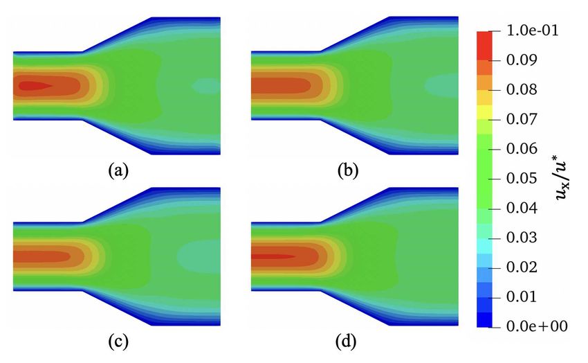
The paper is organized as follows: we introduce the governing equations, namely Stokes equation with a complex-
valued source term, in the spectral domain in Section 2.1. Second, we present the weak and discrete formulations
of those equations based on finite element formulation in Sections 2.2 and 2.3, respectively. Then, we introduce the
SCVS algorithm and elaborate on how to estimate the error in Sections 2.4 and 2.5. Next, we move on to Section
3 where we evaluate the introduced technique using four cases, where we compare the solutions obtained from the
SCVS and a standard RBVMS solver. The convergence and accuracy of the SCVS are established for a canonical case
where an analytical solution is available. The computational efficiency of the SCVS is demonstrated and contrasted
against that of the RBVMS in Section 3.6. Finally, we have a look at possible research directions before drawing
conclusions at the end in Sections 4 and 5 respectively.

2. Complex-valued Stokes solver formulation

   In what follows, we first briefly describe the complex-valued Stokes equation as the governing equation for low
Reynolds number flows, discuss its discrete formulation using FEM, and then present the SCVS algorithm in detail.

2.1. Governing equations
   Consider creeping fluid flow in a domain Ω with boundary Γ = ∂Ω that is governed by the incompressible unsteady
Stokes equations as

                                                     ∂u
                                                    ρ     = −∇p + ∇ · (µ∇u) in Ω,
                                                      ∂t
                                                    ∇ · u = 0 in Ω,                                                        (1)
                                                        u = g on Γg ,
                                        (−pI + µ∇u) · n = h on Γh ,

where u(x, t) refers to the velocity of the fluid at location x and time t, p(x, t) is the pressure, ρ is the density, n is the
boundary Γ outward normal vector, and µ is the viscosity. g and h refer to the imposed velocity and traction on the
Dirichlet Γg and Neumann Γh boundaries where Γ = Γg ∪ Γh . Additionally, suppose that these boundary conditions are
time-periodic with a period of T .
    To represent Eq. (1) in the spectral domain, we make use of
                                                             X
                                                   u(x, t) =    ũi (x)e ĵωi t ,
                                                               i
                                                               X                                                           (2)
                                                   p(x, t) =       p̃i (x)e ĵωi t ,
                                                               i
            √
where ĵ = −1. Here the frequency ωi is defined in terms of period T as ωi = 2πi/T for i = 0, 1, . . . , Nm with Nm
denoting the largest computed mode. For time-periodic flows, such as those encountered in cardiovascular modeling,
T is the cardiac cycle, which is the time it takes for boundary conditions to repeat themselves. Similar to the state vari-
                                                                                                                 P
ables, Dirichlet and Neumann boundary conditions can be expressed in the spectral domain as g(x, t) = i g̃i (x)e ĵtωi t
              P
and h(x, t) = i h̃i (x)e ĵtωi t , respectively. With these definitions, Eq. (1) and continuity equation can be written as

                                                  ĵωi ρũi = −∇ p̃i + ∇ · (µ∇ũi ) in Ω,
                                                    ∇ · ũi = 0 in Ω,
                                                                                                                           (3)
                                                        ũi = g̃i on Γg ,
                                      (− p̃i I + µ∇ũi ) · n = h̃i on Γh .

These equations resemble those of the steady Stokes equation with a nonzero source term. The only difference is that
the first (source) term in Eq. (3) is complex-valued unless ωi = 0, for which the steady Stokes equations in the real
domain are recovered.

                                                               3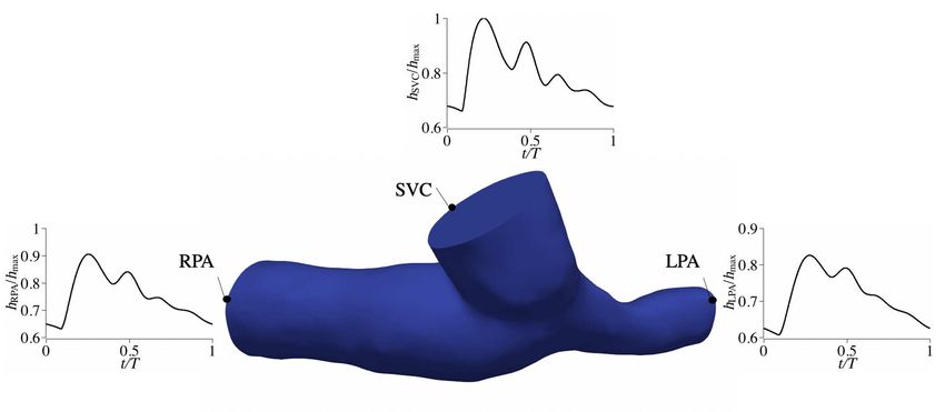
2.2. Weak formulation
    Since the solution to Eq. (3) at ωi and ω j for i , j are independent, we only need to provide a solution procedure at
a single frequency ωi . Thus, for the sake of notation brevity, we drop subscript i and denote our formulation in terms
of variable ω below.
    The weak form of Eq. (3) is stated as follows. Given the frequency ω, find ũ ∈ S and p̃ ∈ P such that for any
w ∈ W and q ∈ Q
                           BG (w, q; ũ, p̃) = FG (w, q) ,
                                               ˆ h                                           i
                                        BG =       ĵωρw · ũ + ∇w : (− p̃I + µ∇ũ) + q∇ · ũ dΩ,
                                                                                                                      (4)
                                               ˆΩ
                                       FG =       w · h̃dΓ,
                                               Γh

holds. In Eq. (4), w and q are test functions for velocity and pressure, respectively, and
                                               n                                   o
                                           S = ũ|ũ(x) ∈ (H 1 )nsd , ũ = g̃ on Γg ,
                                               n                                    o
                                         W = w|w(x) ∈ (H 1 )nsd , w = 0 on Γg ,
                                               n             o                                                        (5)
                                           P = p̃| p̃(x) ∈ L2 ,
                                               n             o
                                           Q = q|q(x) ∈ L2 .

   are velocity and pressure solution and test function spaces. L2 denotes the space of scalar-valued functions that are
square-integrable on Ω, and (H 1 )nsd denotes the space of vector-valued functions with square-integrable derivatives on
Ω.

2.3. Discrete formulation
    Denoting the finite-dimensional subspace of S, W, P, and Q by Sh , W h , Ph , and Qh , respectively, we attempt to
solve the discrete form of Eq. (4) using Galerkin’s approximation. Namely, we seek ũh ∈ Sh and p̃h ∈ Ph such that
for any w̃h ∈ W h and q̃h ∈ Qh
                                          BG wh , qh ; ũh , p̃h = FG wh , qh ,                                   (6)
holds. In writing Eq. (6), we assumed Ωh = Ω, i.e., the computational domain after discretization remains unchanged.
If the two differ, then one must perform the integrals over Ωh rather than Ω when computing BG and FG in Eq. (6).
     Galerkin’s formulation of incompressible flow has a saddle-point nature, which produces a singular system if one
were to adopt similar shape functions for velocity and pressure. Various techniques have been proposed to overcome
this issue, ranging from mixed-element [19] and penalty techniques [20] to stabilized finite element methods [21]. In
the present study, we adopt the mixed finite element method, which allows us to reduce the number of variables that
influence the accuracy of the SCVS formulation, thus simplifying the measurement of its numerical properties. More
specifically, we employ linear and quadratic shape functions for pressure and velocity, respectively, to satisfy inf-sup
condition (also known as LBB condition) [22, 23, 24]. In 2D and 3D, we use linear triangular and tetrahedral elements
with 3 and 4 nodal points, respectively, for pressure. For velocity, we use quadratic shape functions that produce 6
and 10 nodes in each of the aforementioned elements in 2D and 3D, respectively. Denoting these linear and quadratic
shape functions at global node A by NA (x) and MA (x) , respectively, the test functions and unknowns are interpolated
in space using
                                                 X
                                       wh (x) =        MA (x)W A ,
                                                    A∈η\ηg
                                                    X
                                         h
                                        q (x) =            NA (x)QA ,
                                                    A∈η̂
                                                     X                    X                                           (7)
                                        ũh (x) =            MA (x)UA +          MA (x)GA ,
                                                    A∈η\ηg                A∈ηg
                                                    X
                                         h
                                        p̃ (x) =           NA (x)PA ,
                                                    A∈η̂

                                                                  4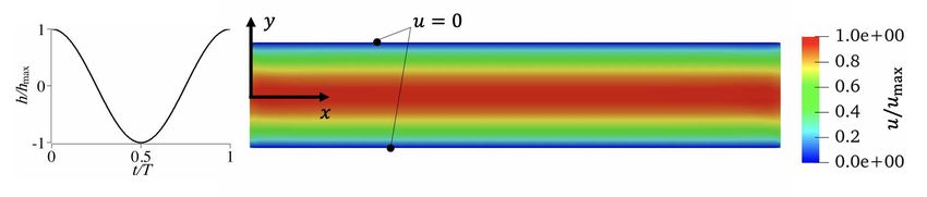
where η, ηg , and η̂ refers to the velocity nodes, velocity nodes on the Dirichlet boundaries, and pressure nodes,
respectively. U A , PA , W A , QA in Eq. (7) are the velocity and pressure unknowns and their respective test functions. GA
is the prescribed velocity defined on the Dirichlet boundaries after discretization such that
                                                                    X
                                               g̃h (x) = Πh g̃(x) =    MA (x)GA ,                                        (8)
                                                                       A∈ηg

where Πh g̃ is an operator that projects g̃ to the finite-dimensional discrete space.
   Substituting for the variables appearing in Eq. (6) using Eq. (7) while ensuring the results holds for any W A and
QA produces the following system of linear equations

                                                               AX = R,                                                  (9)

where                                         "             #        " #           " #
                                            K             D           U             B
                                         A= T                 ,   X=     ,      R=     ,                               (10)
                                            D             0           P             0
and K and D matrices and B vector are computed as
                                         ˆ
                                  K AB =     ĵωρMA MB + µ∇MA · ∇MB IdΩ,
                                          Ω
                                          ˆ
                                  DAB = − ∇MA NB dΩ,                                                                   (11)
                                         ˆ Ω
                                    BA =    MA h̃dΓ − K AB GB .
                                                  Γh

The solution to this linear system is obtained using a brute-force approach. Namely, we treat the entire linear system
as a single sparse matrix and solve it iteratively using the Generalized minimal residual method (GMRES) method
[25] with a Jacobi preconditioner. All these methods are implemented in our in-house linear solver that employs
an optimized data structure for scalable distributed parallel processing [26]. The GMRES algorithm used for this
purpose is slightly modified from its real counterpart owing to K being complex-valued. The same linear solver and
preconditioner are also used for the RBVMS to allow for a one-to-one comparison of computational cost between
the two. This choice has been made due to the underlying structure of the tangent matrix, which is not symmetric
for the RBVMS, as well as its relative simplicity and wider use by the finite element community. Provided that the
left-hand side matrix in the case of SCVS is symmetric and has a block structure, one may adopt a linear solution
and preconditioning strategy based on Schur complement to reduce the overall cost of solving this linear system in
the future [27, 28, 29, 30]. The use of multigrid [31] is also expected to significantly reduce the cost of linear solve,
particularly on finer grids.

2.4. SCVS algorithm
    In this section, we discuss the implementation of the SCVS algorithm. Overall, the procedure involves representing
the boundary conditions in the spectral domain, then solving for flow at each mode, and reconstructing the solution in
the real domain.
   1. Take the Fourier transformation of the boundary conditions g(x, t) and h(x, t) as

                                                                 1 T
                                                                  ˆ
                                                       g̃i (x) =     g(x, t)e− ĵωi t dt,
                                                                 T 0
                                                                                                                       (12)
                                                                 1 T
                                                                  ˆ
                                                       h̃i (x) =     h(x, t)e− ĵωi t dt.
                                                                 T 0
   2. Select the number of modes to truncate the above series based on the smoothness of the boundary conditions.
      Note that the number of required modes can be determined directly from the frequency content of the prescribed
      boundary conditions due to the linearity of the Stokes equations.
                                                                   5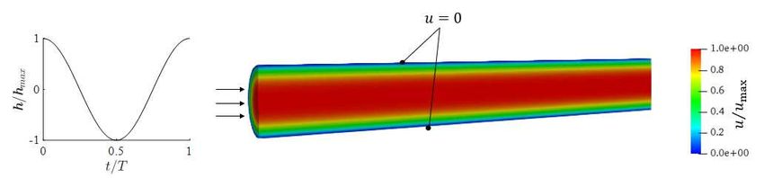
More specifically, one can select a tolerance ǫm to obtain a priori estimate of the number of required modes
      Nm + 1 such that
                                               2
                                                    kh − ĥk2L2 (Γh ×T ) kg − ĝk2L2 (Γg ×T )
                                              eM =                        +                      < ǫm2 ,                        (13)
                                                      khk2L2 (Γh ×T )          kgk2L2 (Γg ×T )
                         P Nm                                  P Nm
      in which ĥ(x, t) = i=0  h̃i (x)e ĵωi t and ĝ(x, t) = i=0     g̃i (x)e ĵωi t are the truncated Neumann and Dirichlet bound-
                                                                                ´T P                                    ´T P
      ary conditions using Nm +1 Fourier modes and khk2L2 (Γh ×T ) = t=0 Γi ∈Γg khk2L2 (Γi ) dt and kgk2L2 (Γg ×T ) = t=0 Γi ∈Γg kgk2L2 (Γi ) dt.
      Even though we are selecting the first Nm modes to truncate the series in this study, in general one may select a
      non-consecutive set of modes solely based on their amplitude to accelerate the rate of convergence.
   3. Construct and solve the linear system in Eq. (9) for ω0 , ω1 , . . . , and ωNm given the boundary conditions computed
      from the previous step, i.e., g̃i (x) and h̃i (x).
   4. Given the solution U A and PA , reconstruct the solution in the spectral domain using Eq. (7) and then in time as
                                                                        X
                                                                        Nm
                                                          uh (x, t) =         ũhi (x)e ĵωi t ,
                                                                        i=0
                                                                                                                                  (14)
                                                                        X
                                                                        Nm
                                                           h
                                                          p (x, t) =          p̃hi (x)e ĵωi t ,
                                                                        i=0

    The number of computed modes Nm + 1, which was selected based on a priori error estimate, can be refined
following the computation of each solution mode. This way, one can compute the difference between the solutions
computed from Eq. (14) using Nm − 1 and Nm modes and decide whether to continue computing the next mode if that
difference is larger than a prespecified tolerance.
    This flexibility presents a significant advantage over the conventional spatio-temporal techniques where capturing
an additional mode requires repeating the entire simulation.
    Later in Section 3.5, we will show the rate at which a priori (Eq. (13)) and a posteriori (Eq. (15)) errors drop as
Nm increases are the same, implying that one can simply rely on Eq. (13) to select Nm . In our experience, Nm ≤ 7 is
typically sufficient for cardiovascular applications where the boundary conditions are smooth and periodic in time.

2.5. Error estimation
    To ensure consistency and accuracy of the proposed formulation, we will consider a set of canonical cases where
an analytical solution to the governing equations is available. The overall error of a conventional scheme stems
from spatial discretization error, the linear solver error, time integration error, and in the case of nonlinear equations,
Newton-Raphson iteration error. If we consider the solution at a single mode, i.e., boundary conditions oscillating at
a single frequency, then SCVS is only prone to the first two types of error enumerated above (discretization and linear
solver). Thus, in what follows, we establish the overall accuracy of the SCVS algorithm as the mesh size or linear
solver tolerance is varied. Also, for scenarios in which the boundary conditions are generic functions of time, we will
study the convergence of the SCVS solution as a function of Nm .
    The overall error e(t) is defined based on the relative difference between the computed velocity uh (x, t) and the
reference velocity u(x, t) over the domain Ω as

                                                          ku(x, t) − uh (x, t)kL2 (Ω)
                                                 e(t) =                               ,                                           (15)
                                                               ku(x, t)kL2 (Ω)

where the L2 (Ω) norm is defined as kuk2L2 (Ω) = Ω u · udΩ. As discussed earlier, this total error can be decomposed
                                                   ´

to the error due to spatial discretization eH and the error due to the linear solver eL . Denoting the best approximation
of the solution in the finite dimensional solution space Sh by Πh u, L2 -norm of the interpolation error for the quadratic
shape functions employed here can be estimated as [32]

                                                      ku − Πh ukL2 (Ω)          kukH 3 (Ω)
                                           eH (t) =                    6 C 1 h3            ,                                      (16)
                                                         kukL2 (Ω)              kukL2 (Ω)
where C1 is a constant and h is the diameter of the smallest element-bounding circle in 2D and sphere in 3D.
                                                                   6
The error related to the linear solver eL is produced by the approximate nature of the iterative solution procedure
employed in solving Eq. (9). This error can be related to the linear solver tolerance ǫL as
kR − A b
Xk2
eL (t) = C2 ≤ C2 ǫL , (17)
kRk2
in which bX is the approximate solution obtained from the iterative linear solver. In Eq. (17), the constant C2 depends
on the inverse of tangent matrix A−1 from Eq. (10) and thus is independent of the boundary conditions. How the
overall error e changes with eH and eL for a pipe flow will be investigated in Section 3.4.
3. Results
The solution procedure and four case studies selected for evaluating the SCVS algorithm are discussed in this
section. To establish the relative accuracy and cost of the SCVS, we will compare it against a standard RBVMS solver.
The details pertaining to the RBVMS algorithm are included in Appendix A. The four test cases considered in this
study are (1) a 2D channel, (2) a 2D diverging nozzle, (3) a 3D pipe, (4) a patient-specific model of Glenn procedure
with an anastomosis [33]. Since the analytical solution is available for the first and third cases, these two cases will
be employed to validate our implementation and evaluate its numerical characteristics. While the boundary conditions
are periodic and contain a single frequency for those two cases, they are generic functions of time for the case two and
four, thus allowing us to study the convergence of solution with regard to Nm and its relationship to eM . At the end of
this section, the performance of the SCVS and the RBVMS are compared in terms of total CPU time and wall-clock
time to demonstrate the performance of the SCVS.
The SCVS uses mixed quadratic-linear shape functions for velocity and pressure, respectively, whereas the RB-
VMS uses linear shape functions for both. This incompatibility raises a concern that comparing the two is similar
to comparing apples to oranges. To address this concern, we have implemented a Stokes solver with mixed shape
functions (called MSS) that is identical to the SCVS except for the traditional discretization of the acceleration term
in the time domain. The formulation of the MSS along with its performance metrics relative to the SCVS and the
RBVMS are included in Appendix B, where we also explain why the SCVS is solely compared against the RBVMS
for the remainder of this article.
3.1. Solution procedure
The 2D and 3D models are initially discretized using triangular and tetrahedral elements. For this purpose, we use
a combination of Tetgen [34] and Simvascular [35] software. An in-house script was developed to generate quadratic
elements from the linear triangular and tetrahedral elements through a node insertion process. For boundary nodes,
special care was taken to ensure that inserted nodes are properly projected to be located on the curved boundaries.
Since the SCVS simulations are performed using quadratic and the RBVMS using linear elements, we reduce the
number of elements for the quadratic meshes such that the total number of degrees of freedom is roughly the same as
the linear meshes, thus allowing for a one-to-one comparison between the two. A zero initial condition is used for all
the RBVMS simulations. The generalized-α method is used for time integration of the RBVMS, which is an implicit
second-order method [36]. As detailed in Appendix A, despite some similarities with the operator splitting techniques
[37], velocity and pressure are solved together during each linear solve. The time step size for the RBVMS is selected
to sufficiently resolve the time variation of boundary conditions. More specifically, we employ 2,000 time steps for
cases with time-varying boundary conditions. For the steady simulations, the time step size is selected such that the
diffusive Courant–Friedrichs–Lewy (CFL) number ∆tν/h2 = 1. The time integration is continued for steady cases
until the relative residual falls below 10−6 . A total of five cycles are simulated to achieve cycle-to-cycle convergence
for the RBVMS simulations. All the results shown below correspond to the last simulated cycle.
For all cases, the Reynolds number is Re < 10−3 to ensure nonlinear effects are negligible in the case of RBVMS
solver. The Reynolds number is defined based on the maximum flow rate through boundaries, the area of the boundary
with the maximum flow rate, and the kinematic viscosity ν = µ/ρ. We only perform a single Newton-Raphson iteration
in the RBVMS simulations, given that the governing equations are linear.
The GMRES method is adopted for solving the resulting linear system for both the SCVS and RBVMS using the
same tolerance ǫL = 10−6 . We used our in-house linear solver for this purpose [30, 29, 26]. As discussed earlier, the
7linear system in the case of the SCVS is complex-valued, requiring us to make a necessary adjustment to the real-
valued version of our GMRES solver to accommodate for a complex-valued linear system. Both the RBVMS and the
SCVS solvers are also implemented in our in-house finite element solver, which is written in object-oriented Fortran
and parallelized using the MPI library.
3.2. 2D channel flow
A 2D channel with a length-to-height aspect ratio of 5 is considered as our first case study (Fig. 1). The geometry
is discretized using 3,762 linear triangle elements for the RBVMS solver and 882 quadratic elements for the SCVS
solver, producing 2,000 and 1,881 nodes and 6,000 and 4,262 degrees of freedom for two cases, respectively. The
non-slip boundary condition is imposed for the top and bottom walls. Either a nonzero constant or a cosinusoidal
Neumann boundary condition is imposed on the inlet, and zero traction is imposed at the outlet. These boundary
conditions produce a solution that corresponds to the fully developed condition observed in an infinitely long channel
(i.e., pressure gradient does not vary as a function of x). The amplitude of the wave, which otherwise is irrelevant due
to the linearity of the Stokes equations, is selected such that the Reynolds number is sufficiently small for the RBVMS
computations. The oscillation frequency ω is varied to simulate a wide range of conditions. More specifically, the
Womersley number W = ωH 2 /ν with H denoting the half-channel height varies from 0 to 20π for the results shown
below.
Figure 1: The schematic of the simulated 2D channel flow. A cosinoidal Neumann boundary condition is imposed at the inlet. The shown contour
is normalized velocity magnitude at t = T/4 for W = 2π case obtained from the SCVS.
An analytical solution is available for the oscillatory flow in the 2D channel, expressed in the spectral domain as a
function of local height y and ω according to [38]
h̃ x
(H + y)(H − y), ω = 0,
2µL
ũ x (y, ω) =
(18)
ĵh̃ x y
− 1 − cosh (Λ)−1 cosh Λ , ω , 0,
ρLω H
where Λ2 = ĵW, ũ x is the streamwise velocity in the spectral domain, L is the channel length, and h̃ x is the traction
amplitude at ω imposed at the inlet acting in the streamwise direction. This solution can also be expressed in time as
n o
u x (y, t) = real ũ x (y, ω)e ĵωt . (19)
The SCVS and the RBVMS simulation results are compared against the analytical solution for W = 2π, W = 10π,
and W = 20π at two time points t = T/4 and t = T/2 in Fig. 2. In general, the error increases as the flow becomes more
oscillatory (at higher W). This larger error can be attributed to the velocity profile developing sharper gradients near
the walls. At a similar W and time point, the SCVS provides more accurate predictions in comparison to the RBVMS.
This higher accuracy is despite the fact that a larger number of degrees of freedom were employed in the RBVMS
simulations. The primary reason for this improved accuracy is the use of quadratic shape function for the SCVS. The
time integration scheme and the stabilization terms also contribute to the larger errors in the RBVMS results.
A more condensed version of these results is provided in Table 1, where the relative error at time point T/4 and
T/2 are computed using Eq. (15) for the RBVMS and the SCVS. In the steady case, since the analytical solution
is a parabola and can be exactly represented by the quadratic shape functions, the SCVS error of e = 1.34 × 10⁻⁵
8is solely due to the linear solver. Repeating this computation with a smaller ǫL confirms that e for the SCVS can
be arbitrarily lowered without refining the grid. The steady solution for the RBVMS, on the other hand, shows a
relatively larger error of 1.93% that is grid-dependent given that it utilizes linear shape functions. The same improved
accuracy is observed at higher modes, where for instance, the RBVMS produces a solution with a 13.4% error at T/2
and W = 20π, whereas the SCVS error remains as low as 1.83%. In general, in comparison to the RBVMS method,
the SCVS is an order of magnitude more accurate for a mesh with a similar number of nodes.
1.2 0.2
1 0 analytical
SCVS
-0.2 RBVMS
0.8
-0.4
0.6
-0.6
0.4
-0.8
0.2 -1
0 -1.2
-1 -0.5 0 0.5 1 -1 -0.5 0 0.5 1
1.2 0.2
1 0
-0.2
0.8
-0.4
0.6
-0.6
0.4
-0.8
0.2 -1
0 -1.2
-1 -0.5 0 0.5 1 -1 -0.5 0 0.5 1
1.2 0.2
1 0
-0.2
0.8
-0.4
0.6
-0.6
0.4
-0.8
0.2 -1
0 -1.2
-1 -0.5 0 0.5 1 -1 -0.5 0 0.5 1
Figure 2: Normalized streamwise velocity as a function of channel height y/H obtained from the SCVS (solid black), the RBVMS (dashed red),
and the analytical solution (circles) for the 2D channel flow shown in Fig. 1. The velocity is normalized using analytical umax . The results on the
left and right columns are extracted at t = T/4 and t = T/2, respectively, and those on the first, second, and third row correspond to W = 2π, 10π,
and 20π, respectively.
9Table 1: Comparison of error in the solution obtained from the SCVS and the RBVMS
solver as a function of the Womersley number W computed using Eq. (15) for the 2D
channel flow shown in Fig. (1). The errors and relative figures are in percent.
SCVS (%) RBVMS (%) Relative (%)
W = ωH 2 /ν
e(T/4) e(T/2) e(T/4) e(T/2) T/4 T/2
−3
0 1.3 × 10 1.9 6.9 × 10⁻²
2π 0.01 0.031 0.27 0.40 3.7 7.8
10π 0.12 0.46 0.84 8.0 14 5.7
20π 0.29 1.8 1.3 13 21 14
3.3. 2D diverging nozzle
In the second example, we consider a 2D diverging nozzle with an expansion ratio of 2 (Fig. 3). This geometry
is discretized using 2,400 linear triangle elements for the RBVMS solver and 600 quadratic elements for the SCVS
solver, producing 1,281 nodes in both cases with 5,124 and 4,184 degrees of freedom, respectively. A time-periodic
Neumann boundary condition is imposed on the inlet, and zero traction is imposed on the outlet (Fig. 3).
Figure 3: The schematic of the 2D diverging nozzle geometry. A physiologic time-periodic Neumann boundary condition is imposed on the inlet.
The time variation of the inlet Neumann boundary is selected to resemble a physiologic pressure waveform, with
its time average being set to zero to emphasize the role of unsteady modes in the solution. The top and bottom walls
are considered as non-slip boundaries.
1010-3
10-4
10-5
10-6
10-7
10-8
10-9
100 101 102
Figure 4: The frequency content of the Neumann boundary condition imposed at the inlet of 2D diverging nozzle case shown in Fig. 3.
Even though the inlet Neumann boundary contains a wide range of frequencies, only the first few modes have a
large enough amplitude to have a significant effect on the results. As shown in Fig. 4, k h̃i k follows a power-law trend
versus ωi , experiencing a sharp drop that is approximately proportional ω−2 i . Such a sharp drop in the amplitude at
higher frequencies justifies the truncation of the series at a relatively low wavenumber. Thus, to construct the SCVS
solution, we select Nm = 5 and solve for ω1 , . . . , ω5 while neglecting ω0 given the time-average of the inlet boundary
condition is zero. The Womersley number, i.e., W = ωH 2 /ν with H being the half-inlet height, for these simulated
modes ranges from 0 to 10π. To show the convergence of SCVS solution with Nm , we reconstructed solution at t = T
using one (Nm = 1), three (Nm = 3), and five (Nm = 5) modes. The results of these computations normalized by
u∗ = |h̃ x (ω = 1)|H/µ for Nm = 1, 3, and 5 are shown in Fig. 5 along with the results obtained from the RBVMS. This
figure shows the qualitative convergence of the SCVS at Nm = 3.
Figure 5: Velocity in the x-direction for 2D diverging nozzle shown in Fig. 3 at t = T computed using the RBVMS (a) and the SCVS (b-d) with
Nm = 1, 3, and 5, respectively.
For a more quantitative comparison of two formulations, the dimensionless flow rate Q/Q∗ , with Q∗ = Hu∗ being
the characteristic flow rate, is computed and shown in Fig. 6 for the RBVMS and the SVC with Nm = 1, 3, and 5.
11Taking the flow computed from the SCVS solution with Nm = 10 as the reference, the relative error in the prediction of
the RBVMS is 1.0%, whereas the relative error for the SCVS at Nm = 1, 3, and 5 is 25%, 5.0%, and 1.5%, respectively.
The fast rate of convergence of the SCVS with respect to Nm confirms our earlier argument that only a few modes are
needed to obtain a converged solution using the SCVS algorithm when boundary conditions vary smoothly in time.
0.1
0
-0.1
-0.2
-0.3
0 0.2 0.4 0.6 0.8 1
Figure 6: Normalized flow rate for the case shown in Fig. 3 obtained from the RBVMS (dashed red) and the SCVS with Nm = 1 (dotted black), 3
(dashed-dot black), and 5 (solid black).
3.4. 3D Pipe flow
For the third case study, we consider an oscillatory laminar pipe flow. A pipe with an aspect ratio of L/R = 15 is
considered with a cosinusoidal inlet and zero outlet Neumann boundary condition (Fig. 7). Similar to the 2D channel
flow case in Section 3.2, these boundary conditions produce a solution that corresponds to the fully developed condition
observed in an infinitely long pipe. The oscillation period is varied to simulate flow at eleven Womersley numbers
W = ωR2 /ν = 0, 8π, . . . , 80π with R denoting the radius of the pipe. As we discussed earlier, the domain is discretized
in space using linear and mixed quadratic-linear tetrahedral elements for the RBVMS and the SCVS simulations,
respectively. A wide range of meshes is constructed to investigate the convergence of both solvers (Table 2). The
number of elements in corresponding meshes is selected such that the number of nodes is roughly the same for both
solvers. Overall, the element size normalized by the pipe radius varies from 0.0340 to 0.228 among simulated cases.
Table 2: Meshes used for discretization of the 3D pipe flow case shown in Fig. 7. QM and LM refer to mixed quadratic-linear
and linear tetrahedral meshes, which are employed in the SCVS and the RBVMS simulations, respectively. Nele , Nnds , and
Ndof denote the numbers of elements, nodes, and degrees of freedom, respectively.
SCVS RBVMS
Mesh
QM1 QM2 QM3 QM4 LM1 LM2 LM3 LM4
Nele 24,450 49,388 95,524 162,444 207,063 374,852 728,922 1,197,044
Nnds 37,469 70,872 133,645 225,610 37,401 64,434 122,291 197,660
Ndof 113,193 221,894 418,400 705,311 149,604 257,736 489,164 790,640
12Figure 7: Schematic of the simulated oscillatory laminar flow in a pipe. h(t)/hmax is the time trace of the imposed Neumann boundary condition at
the inlet. The contour of normalized radial velocity magnitude is shown for W = 8π case at t = T/4 obtained from the SCVS solver.
Similar to the first case considered above, an analytical solution is available for this case that permits us to establish
the accuracy of each solver. For an oscillatory flow in a pipe, the solution in the spectral domain is expressed as [39]
h̃ x 2
(R − r2 ), ω = 0,
4µL
ũ x (r, ω) =
(20)
ĵh̃ x r
− 1 − J0 (Λ)−1 J0 (Λ ) , ω , 0,
ρLω R
where Λ2 = − ĵW and J0 is the zero order Bessel function of the first kind. This solution can be expressed in time
using n o
u x (r, t) = real ũ x (r, ω)e ĵωt . (21)
For a qualitative evaluation of the SCVS and the RBVMS solutions, simulated u x (r, T/4) and u x (r, T/2) along with
the analytical prediction of Eq. (21) at W = 8π, 40π, and 80π are shown in Fig. 8. These results are obtained using the
finest grids, namely QM4 and LM4 in Table 2. Similar to what we observed earlier in Section 3.2 for the 2D channel
flow, the SCVS provides a better approximation, particularly at larger Womersely numbers or at t = T/2, in which
the solution exhibits sharper gradients. The error in the steady state solution (W = 0) obtained from the RBVMS and
SCVS solver using the finest grids is e = 9.0 × 10⁻³ and e = 1.4 × 10⁻⁴ , respectively. The superior accuracy of the
SCVS, which is achieved despite using fewer degrees of freedom, is primarily a result of utilizing a higher-order shape
function. The numerical integration and stabilization terms are the secondary contributors to the larger error in the
case of the RBVMS.
131.2 0.2
1 0
-0.2
0.8
-0.4
0.6
-0.6
0.4 analytical
-0.8
SCVS
0.2 -1 RBVMS
0 -1.2
-1 -0.5 0 0.5 1 -1 -0.5 0 0.5 1
1.2 0.2
1 0
-0.2
0.8
-0.4
0.6
-0.6
0.4
-0.8
0.2 -1
0 -1.2
-1 -0.5 0 0.5 1 -1 -0.5 0 0.5 1
1.2 0.2
1 0
-0.2
0.8
-0.4
0.6
-0.6
0.4
-0.8
0.2 -1
0 -1.2
-1 -0.5 0 0.5 1 -1 -0.5 0 0.5 1
Figure 8: Normalized velocity profiles as a function of radius for an oscillatory laminar pipe flow (shown in Fig. 7) predicted using the SCVS (solid
black), the RBVMS (dashed red), and analytical solution (circles). The results on the left and right columns are extracted at t = T/4 and t = T/2,
respectively, and those on the first, second, and third row correspond to W = 8π, 40π, and 80π, respectively. Computations are performed on QM4
and LM4 grids for the SCVS and the RBVMS, respectively. All the results are normalized using the maximum velocity from the analytical solution
umax .
To study mesh convergence, the error e(T/2) defined in Eq. (15) is computed for the SCVS and the RBVMS as a
function of h at W = 8π (Fig. 9). Third-order accuracy is observed for the SCVS, indicating that the measured error is
dominated by the discretization error eH . This third order accuracy is in agreement with the estimate in Eq. (16), which
also predicted eH ∝ h3 . A similar relationship can be obtained for the RBVMS, which utilizes linear shape functions,
as
kukH 2 (Ω)
eH 6 C 3 h 2 . (22)
kukL2 (Ω)
The second-order accuracy of RBVMS is also confirmed by the results shown in Fig. 9.
1410-1
10-2
10-3
RBVMS
SCVS
0.03 0.06 0.09 0.12 0.15
Figure 9: The relative error e (defined in Eq. (15)) at t = T/2 as a function of element size for the oscillatory pipe flow shown in Fig. 7 at W = 8π.
The shown data correspond to the SCVS (solid black circles), the RBVMS (hollow red circles), the analytical estimate of the SCVS error from
Eq. (16) (solid black line), and the analytical estimate of the RBVMS error from Eq. (22) (dashed red line).
To further analyze each method’s accuracy for various flow conditions, we next study the overall error as a function
of the Womersley number W. As we observed earlier in Figs. 2 and 8, the velocity profile develops sharper gradients
near the wall at higher modes, thereby producing a larger error at higher W. That qualitative observation is confirmed
quantitatively in Fig. 10 that shows a direct power-law relationship between e and W. This relationship indicates that
resolving the velocity field at higher modes requires improved spatial resolution. It also shows that the quality of the
solution degrades faster for quadratic elements than the linear elements as W increases. In what follows, we explain
these observations in more detail and analytically predict the exponents that appear in the power-law relationship
between e and W for the RBVMS and SCVS.
10-1
10-2
RBVMS
10-3 SCVS
50 150 250
Figure 10: The relative error e (defined in Eq. (15)) at t = T/2 as a function of the Womersley number W for the oscillatory pipe flow shown
in Fig. 7. The shown results correspond to the SCVS using QM4 grid (solid black circles), the RBVMS using LM4 grid (hollow red circles), the
analytical estimate of the SCVS error from Eqs. (16) and (25) (solid black line), and analytical estimate of the RBVMS error from Eqs. (22) and (25)
(dashed red line).
Since the linear solver tolerance ǫL is selected to be sufficiently small in this case and eL is negligible in comparison
to eH , we can explain e ∝ W 3/2 for the SCVS and e ∝ W for the RBVMS by further analyzing the behavior of eH for
each solver. To utilize Eqs. (16) and (22) for this purpose, we first need to establish how kukL2 , kukH 2 , and kukH 3 vary
15with W. Considering only cases in which W , 0 and the fact that u x = u x (r, t), from Eq. (20) we can write
ˆ !1/2 ˆ R !1/2
h̃ x
kukL2 = u2x dΩ = 2πrz1 z̄1 dr ,
Ω ρω r=0
!2 ˆ R !1/2
∂2 u x h̃ x Λ
kukH 2 = = 2πrz2 z̄2 dr , (23)
∂r2 L2 ρw R r=0
!3 ˆ R !1/2
∂3 u x h̃ x Λ
kukH 3 = = 2πrz3 z̄3 dr ,
∂r3 L2 ρw R r=0
h i
where z1 (r; Λ) = 1 − J0 (Λ)−1 J0 (Λ Rr ), z2 (r; Λ) = J2 (Λ Rr ) − J0 (Λi Rr ) /(2J0 (Λ)),
h i
z3 (r; Λ) = 3J1 (Λ Rr ) − J3 (Λ Rr ) /(4J0 (Λ)), and z̄1 denotes complex conjugate of z1 . Neglecting the dependence of these
norms on the integrals of z1 , z2 , and z3 , it is straightforward to show that
h̃ x R4
kukL2 ∝ ,
µW
h̃ x R2
kukH 2 ∝ , (24)
µ
h̃ x R 1
kukH 3 ∝ W2,
µ
indicating kukL2 , kukH 2 , and kukH 3 should vary proportional to W −1 , W 0 , and W 1/2 . Comparing these approximate
predictions against reference quantities (obtained from 1D numerical integration of Eq. (23)) show that all exponents
are over-predicted by 0.2 (Fig. 11). The ratio of these norms, however, is correctly predicted using Eq. (24) as
kukH 2 kukH 3
∝ R−1 W, and ∝ R−3 W 3/2 , (25)
kukL2 kukL2
indicating that the RBVMS and the SCVS error should grow proportional to W and W 3/2 at sufficiently small ǫL owing
to Eqs. (16) and (22), respectively. These analytical predictions are in agreement with our numerical results that were
shown earlier in Fig. (10).
100
10-1
10-2
10-3
10-4
40 120 200
Figure 11: L2 (circles), H 2 (squares), and H 3 (triangles) norms of the analytical solution u for an oscillatory flow in cylinder as a function Womersley
number W. The symbols are obtained by 1D numerical integration of Eq. (23) whereas the lines with given slopes are curve fits.
Next, we investigate the effect of linear solver tolerance ǫL on the overall accuracy of the SCVS, utilizing QM4
mesh and the solution corresponding to W = 8π evaluated at t = T/2. The left and right tail of the results shown in
16Fig. 12 indicate that the overall error e is independent of eL for sufficiently small eL and proportional to ǫL when eL
is sufficiently large. This observation confirms that (as expected) the overall error is dominated by the discretization
error eH and that of the linear solver eL at small and large ǫL , respectively. The transition between dominance of eH
and eL occurs at approximately ǫL = 10−6 , which is a value specific to this case study and a function h among others.
Note that this tolerance is the optimal tolerance with regard to the computational cost, as further decrease in ǫL is not
met with an improved overall solution accuracy. Lastly, note that the slope of 1 observed on the right tail of Fig. 12 is
in agreement with Eq. (17), which predicts eL ∝ ǫL .
100
10-1
10-2
10-3
10-8 10-6 10-4
Figure 12: The overall relative error in the SCVS solution e(T/2) as a function of the linear solver tolerance ǫL . The case considered here corresponds
to an oscillatory pipe flow shown in Fig. 7 at W = 8π and using QM4 mesh. A line with a slope 1 is shown for the reference.
If we take the main objective of designing a computational method to be making a viable prediction at a specified
accuracy with the lowest cost possible, then it is desirable to compare the SCVS and the RBVMS methods on an
error-versus-cost plot. Thus, we have extracted the cost (in terms of CPU time) and error (in terms of e(T/2)) for all
the simulations performed in this section using various grids and W. The results are shown in Fig. 13. Comparing the
symbols with the same color, i.e., for a flow at a given W, the SCVS always provides more accurate predictions at a
lower cost. Focusing on W = 80π cases (blue symbols), the SCVS yields a similar accuracy at the coarsest grid (solid
triangle) to that of the RBVMS at the finest grid (hollow circle) while reducing the cost by three orders of magnitude.
If one holds the computational cost relatively similar (solid blue circle versus hollow blue triangle, for instance), the
SCVS offers over an order of magnitude improvement in accuracy relative to the RBVMS.
17100
10-1
10-2
10-3
10-4
100 101 102 103 104
Figure 13: Relative error e(T/2) as a function of the computational cost tC for the 3D pipe flow example shown in Fig. 7. Symbols with the same
color should be compared. The solid symbols correspond to the SCVS and hollow to the RBVMS. The circle, square, diamond, and triangle symbols
correspond to QM4/LM4, QM3/LM3, QM2/LM2, and QM1/LM1 meshes listed in Table 2. The black, red, and blue colors correspond to W = 8π,
40π, and 80π, respectively. These results show that the SCVS, compared to the RBVMS, always provides a higher accuracy at a lower cost.
3.5. 3D patient-specific Glenn
For the last test case, we will consider a complex patient-specific geometry acquired from a patient undergoing
Glenn operation [33]. As shown in Fig. 14, the superior vena cava (SVC) is anastomosed to the left pulmonary artery
(LPA) and right pulmonary artery (RPA) in this operation. The geometry is discretized using 988,747 linear tetrahedral
elements for the RBVMS solver and 132,066 quadratic tetrahedral elements for the SCVS. This discretization results
in 163,791 and 183,708 nodes and 655,164 and 574,401 degrees of freedom for the linear and quadratic meshes,
respectively. The boundary conditions are selected based on physiologic data and a Windkessel model [3, 40] for the
RPA and LPA faces (Fig. 14). The wall is considered a non-slip boundary.
Figure 14: The geometry and boundary conditions employed for the patient-specific case study. hmax denotes the maximum value of traction
imposed on the SVC.
In this example, twelve modes (Nm = 11) are simulated in total for the SCVS. The case with Nm = 11 is used
as the reference to measure error for the remaining cases, given that the solution accuracy of the SCVS was superior
to that of the RBVMS based on the cases discussed earlier. The Womersley number W = ωD2h /ν is based on the
hydraulic diameter of the SVC (Dh ), which is defined such that πD2h /4 is equal to the area of the SVC boundary. This
18definition, which is the square of what is normally defined in the literature as Womersley number, leads to W = 0,
146π, 293π, . . . , 1611π for simulated ω0 , ω1 , ω2 , . . . , ω11 . The results of these computations are normalized by
u∗ = |h̃SVC (ω = 0)|Dh /µ and Q∗ = πD2h u∗ /4.
A closer examination of the solutions associated with each mode shows that their spatial distribution widely varies
as W increases (Fig. 15). While the velocity peaks at the center of the vessels for the steady solution (Fig. 15-(a)), it
develops two peaks closer to the walls at a larger W. This behavior resembles the trend that we observed earlier in the
canonical geometries (e.g., cylinder in Section 3.5). This behavior is a result of a change in the relative importance of
various terms that appear in the Stokes equation. While only the viscous and pressure terms are active at W = 0, three
terms (acceleration, pressure, and viscous) balance each other for W > 0. As W increases, the relative importance of
the acceleration term increases, leading to a solution that exhibits peaks near the walls rather than at the center of the
geometry.
Figure 15: The velocity magnitude normalized by u∗ obtained from the SCVS solver at t = T/2 for (a) W = 0, (b) W = 146π, (c) W = 293π, (d)
W = 439π, (e) W = 586π, (f) W = 732π, (g) W = 879π, (h) W = 1025π, (i) W = 1171π, (j) W = 1318π, (k) W = 1464π, (l) W = 1611π.
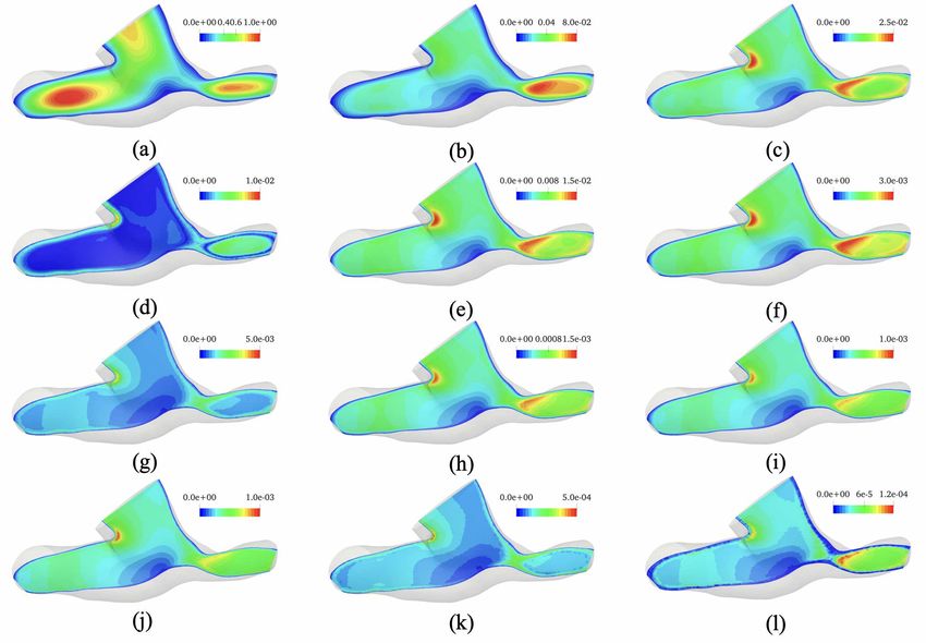
The SCVS solution in the time domain is reconstructed using Eq. (14) and qualitatively compared against that
of the RBVMS (Fig. 16). This qualitative comparison shows that a few modes (in this case 6, including the steady
solution) are sufficient for resolving the solution in this complex geometry.
19Figure 16: Normalized velocity magnitude at t = 1/2T obtained from the SCVS with Nm = 5 (top) and the RBVMS (bottom) for the case shown in
Fig. 14.
For a more quantitative comparison between the SCVS and the RBMVS solutions, the predicted flow through
three branches is shown in Fig. 17. This figure confirms that the difference between the two solvers’ solution reduces
as more modes are employed. Using the case with Nm = 11 as a reference, the relative errors of flux computed from
the RBVMS are 0.65%, 0.38%, and 0.34% on the SVC, LPA, and RPA, respectively. The relative errors in the SCVS
solution with Nm = 7 are 0.14%, 0.19%, and 0.12% for the SVC, LPA, and RPA, respectively. Note that, due to the
error in the RBVMS solution (as well as discretization error in the SCVS), the two solutions do not converge even at
very large Nm . Nevertheless, the SCVS does converge to a solution as Nm → ∞. The rate of this convergence depends
on the smoothness of the boundary conditions.
Figure 17: Normalized flow rate Q/Q∗ through the SVC (a), LPA (b), and RPA (c) predicted by the RBVMS (dashed red) and the SVC with Nm = 3
(dotted black), Nm = 5 (dashed-dot black), Nm = 7 (solid black) for the case shown in Fig. 14.
The relationship between the smoothness of the boundary condition time variation and the convergence rate of
the SCVS with respect to Nm is demonstrated in Fig. 18. eM from Eq. (13), which measures the truncation error
in the imposed boundary conditions associated with the finite Nm , follows the same trend as the overall error e. As
more modes are included in the solution, the boundary conditions approach their temporal reference profile, thereby
improving the overall accuracy of the SCVS solution. Note that the two trends slightly diverge on the right tail of this
plot. This divergence is an artifact of taking the case with Nm = 11 as the reference when measuring kek, whereas eM
is measured against the reference solution. If the exact solution were available and employed as the reference solution,
then kek for very large Nm would have converged to the larger of discretization eH and linear solver eL errors rather
than going to zero.
2010-1
10-2
10-3
10-4
0 2 4 6 8 10
Figure 18: The overall error ke(t)kL2 ([0,T ]) (solid circles) as a function of Nm for the case shown in Fig. 14, using the case with Nm = 11 as the
reference. The truncation error for the imposed Neumann boundaries eM (red squares) is also shown, which follows the same trend as kek.
3.6. Computational costs
The primary reason for the development of the SCVS algorithm was to obtain a more computationally efficient
solution procedure. We discussed some of the performance metrics of the SCVS algorithm in the discussion pertaining
to Fig. 13. In this section, we provide a more comprehensive account of the performance of these two solvers in terms
of computational costs as well as wall-clock-time for all cases studied above.
For cases with multiple grids, we considered the finest grid in computing performance values. Also, we consider
Nm = 5 for the SCVS as it proved sufficient for sufficiently smooth boundary conditions. Thus, the computational cost
tC for the SCVS is computed as the cumulative cost of simulating the first 6 modes. Its wall-clock-time tW , on the
other hand, is taken as the maximum of the wall-clock-time of those 6 simulated modes since they are embarrassingly
parallelizable. The simulation results presented in Sections 3.2 and 3.4 for the canonical 2D channel and 3D pipe flow
cases were for individual modes. Nevertheless, we consider the sum of the cost of the first six modes for those cases
as well. This choice was made to represent a situation in which the flow in these models is simulated with an arbitrary
boundary condition rather than one with a unimodal oscillation. Furthermore, note that both tC and tW for the RBVMS
scale linearly with the total number of time steps1 . The results reported here are what is considered typical, namely
simulating five cycles with each including 2,000 time steps for a total of 10,000 time steps. Finally, the performance
metrics are in general implementation- and machine-dependent. However, given that both the RBVMS and the SCVS
solvers are implemented by our group, written and compiled using the same language and compiler, linked against the
same libraries, and ran on the same machine, the figures in Tables 3 provide an apple-to-apple comparison of the two
formulations.
Table 3: Comparison of the computational performance of the SCVS and RBVMS solvers. Np , tC , tW denote the
number of processors, computational costs in CPU-hours, and the simulation wall-clock-time in hours, respectively.
The last two columns are tC and tW for the SCVS relative to those of the RBVMS. All the SCVS results correspond
to Nm = 5. For cases with multiple grids, we adopted the finest grid in computing these performance figures. The
relative figures are in percent.
SCVS RBVMS Relative (%)
Case
Np tC (hr) tW (hr) Np tC (hr) tW (hr) tC tW
−2 −3
2D channel 6 1.5 × 10 3.9 × 10 16 1.9 0.12 0.79 3.4
2D nozzle 6 7.4 × 10⁻³ 1.8 × 10⁻³ 16 1.0 0.064 0.74 2.9
3D Pipe 384 2.3 × 10² 1.0 64 4.6 × 10³ 72 5.1 1.3
3D Glenn 768 3.2 × 10² 0.52 128 3.0 × 10³ 23 11 2.2
1 Thisstatement applies only to the linear equations considered here, since a large ∆t increases the number of Newton-Raphson iterations at
higher Reynolds numbers, thus changing the cost of advancing the solution for a time step.
21As was hypothesized earlier, the SCVS reduces the overall computational cost significantly when it is compared
against the standard RBVMS formulation. This reduction in cost that ranges from less than 1% for 2D cases to 11% for
the 3D Glenn geometry is primarily achieved by reducing the number of linear solves. While this number is Nm +1 = 6
for the SCVS, it is equal to the total number of time steps for the RBVMS, i.e., 10,000. The performance gap between
the SCVS and RBVMS is not as large as 1667 = 10, 000/6 as a single SCVS linear solver is much more expensive
than that of the RBVMS. On average, the SCVS requires 30,000 GMRES iterations, whereas 500 iterations suffice for
solving the linear system obtained for the RBMVS formulation. The reason for the large number of iterations for the
SCVS is mostly attributed to the high condition number of A matrix that has a zero diagonal sub-block (Eq. (10)). As
discussed in Section 4, reducing the cost of solving this linear solver presents an opportunity for significantly reducing
the cost of the SCVS algorithm in the future.
The performance gap between the SCVS and RBVMS widens when wall-clock time is concerned as tW for the
SCVS is less than 4% of that of the RBVMS for all cases considered here (Table 3). As we discussed earlier, the modes
in the SCVS algorithm are independent and can be solved concurrently. Therefore, the number of processors utilized
in the SCVS computation can far exceed that of the RBVMS without loss of parallel efficiency. Differently put, the
wall-clock time for the SCVS is roughly independent of the number of computed modes as long as there are sufficient
parallel computational resources available. The cumulative effect of this added dimension for parallelization and lower
overall computational cost is a formulation that allows for a much faster turn-around time for a given problem.
4. Future work
The biggest hurdle to be overcome in the future is the extension of the SCVS formulation to high Reynolds number
flows. Such an extension will not be trivial, as one can not exploit the linearity of the governing equations to solve for
velocity and pressure at different modes independently.
Solving for all the modes at the same time will be one way to deal with this coupling. However, this brute
force approach can become quickly unaffordable as the number of modes increases. This limitation, which has been
observed in the past for the Time Spectral Method discussed in Section 1, must be overcome if the extension of SCVS
to the Navier-Stokes equation were to find widespread use in the future.
The efficiency of the SCVS algorithm can be significantly improved in the future by making minor adjustments
in its formulation or its underlying linear solver. Relaxing the incompressibility constraint by using a penalty method
or including stabilization terms in its formulation is expected to reduce the condition of the underlying linear system
significantly. Experimenting with more efficient linear solver algorithms (e.g., bi-partitioned method [30]) as well as
preconditioners [29] can lead to additional improvements in the overall performance of the SCVS algorithm in the
future.
Depending on the hardware architecture, reformulating the problem so that it avoids complex arithmetic may or
may not reduce the cost of this scheme as such reformulation leaves the number of real floating-point operations
unchanged.
5. Conclusions
In this paper, we proposed the SCVS as an alternative approach for fast simulation of time-periodic flow at low
Reynolds numbers in complex geometries. Starting from the unsteady Stokes equation, we showed that it could be
expressed as a steady Stokes equation with an imaginary source term in the time-spectral domain. The resulting
equation can then be discretized and solved as a boundary value problem at a few selected modes, avoiding the use of
costly and unscalable time integration schemes. As a proof of concept, we showed how this boundary value problem
could be solved using Galerkin’s formulation with mixed elements. We later employed this formulation for simulating
flow in a variety of 2D and 3D geometries. To provide a point of reference, all these simulations were also performed
using the standard RBVMS formulation.
For cases with an analytical solution available, the SCVS showed about an order of magnitude improvement in
accuracy relative to the RBVMS at a similar number of degrees of freedom. This difference was attributed to the use
of quadratic shape functions for the SCVS and to a lesser extent to the lack of stabilization terms and time integrator
in our formulation. The variation of the overall error in the SCVS solution as a function of grid size, linear solver
22You can also read