Allometry of behavior and niche differentiation among congeneric African antelopes
←
→
Page content transcription
If your browser does not render page correctly, please read the page content below

15577015, 2023, 1, Downloaded from https://esajournals.onlinelibrary.wiley.com/doi/10.1002/ecm.1549 by University Of Idaho Library, Wiley Online Library on [01/02/2023]. See the Terms and Conditions (https://onlinelibrary.wiley.com/terms-and-conditions) on Wiley Online Library for rules of use; OA articles are governed by the applicable Creative Commons License
Received: 2 November 2021       Revised: 9 June 2022     Accepted: 13 June 2022

DOI: 10.1002/ecm.1549

ARTICLE

Allometry of behavior and niche differentiation among
congeneric African antelopes

Joshua H. Daskin1,2 | Justine A. Becker1,3                                              | Tyler R. Kartzinel4 |
Arjun B. Potter1   | Reena H. Walker5      |                                            Fredrik A. A. Eriksson6                           |
Courtney Buoncore1 | Alexander Getraer1 |                                                  Ryan A. Long5 |                    Robert M. Pringle1

1
 Department of Ecology and Evolutionary
Biology, Princeton University, Princeton,              Abstract
New Jersey, USA                                        Size-structured differences in resource use stabilize species coexistence in ani-
2
 Archbold Biological Station, Venus,                   mal communities, but what behavioral mechanisms underpin these niche dif-
Florida, USA
3
                                                       ferences? Behavior is constrained by morphological and physiological traits
Department of Zoology and Physiology,
University of Wyoming, Laramie,                        that scale allometrically with body size, yet the degree to which behaviors
Wyoming, USA                                           exhibit allometric scaling remains unclear; empirical datasets often encompass
4
 Department of Ecology and Evolutionary                broad variation in environmental context and phylogenetic history, which
Biology, Brown University, Providence,
                                                       complicates the detection and interpretation of scaling relationships between
Rhode Island, USA
5
 Department of Fish and Wildlife
                                                       size and behavior. We studied the movement and foraging behaviors of three
Sciences, University of Idaho, Moscow,                 sympatric, congeneric spiral-horned antelope species (Tragelaphus spp.) that
Idaho, USA                                             differ in body mass—bushbuck (26–40 kg), nyala (57–83 kg), and kudu
6
 Department of Biological Sciences,
                                                       (80–142 kg)—in an African savanna ecosystem where (i) food was patchily dis-
Dartmouth College, Hanover,
New Hampshire, USA                                     tributed due to ecosystem engineering by fungus-farming termites and
                                                       (ii) predation risk was low due to the extirpation of several large carnivores.
Correspondence
                                                       Because foraging behavior is directly linked to traits that scale allometrically
Robert M. Pringle
Email: rpringle@princeton.edu                          with size (e.g., metabolic rate, locomotion), we hypothesized that habitat use
                                                       and diet selection would likewise exhibit nonlinear scaling relationships. All
Funding information
Cameron Schrier Foundation; Greg Carr
                                                       three antelope species selected habitat near termitaria, which are hotspots of
Foundation; High Meadows                               abundant, high-quality forage. Experimental removal of forage from termite
Environmental Institute at Princeton                   mounds sharply reduced use of those mounds by bushbuck, confirming that
University; National Geographic Society,
Grant/Award Number: #9291-13;                          habitat selection was resource driven. Strength of selection for termite mounds
National Science Foundation,                           scaled negatively and nonlinearly with body mass, as did recursion (frequency
Grant/Award Numbers: IOS-1656527,
                                                       with which individuals revisited locations), whereas home-range area and
IOS-1656642, DEB-1501306,
DEB-1930820; Porter Family Foundation                  mean step length scaled positively and nonlinearly with body mass. All species
                                                       disproportionately ate mound-associated plant taxa; nonetheless, forage selec-
Handling Editor: Neil H. Carter
                                                       tivity and dietary composition, richness, and quality all differed among species,

Joshua H. Daskin and Justine A. Becker are joint first authors on this work.

Ryan A. Long and Robert M. Pringle contributed equally to this work.

This is an open access article under the terms of the Creative Commons Attribution License, which permits use, distribution and reproduction in any medium, provided
the original work is properly cited.
© 2022 The Authors. Ecological Monographs published by Wiley Periodicals LLC on behalf of The Ecological Society of America.

Ecological Monographs. 2023;93:e1549.                                                                              https://onlinelibrary.wiley.com/r/ecm       1 of 31
https://doi.org/10.1002/ecm.1549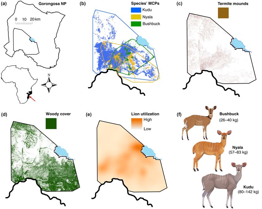
15577015, 2023, 1, Downloaded from https://esajournals.onlinelibrary.wiley.com/doi/10.1002/ecm.1549 by University Of Idaho Library, Wiley Online Library on [01/02/2023]. See the Terms and Conditions (https://onlinelibrary.wiley.com/terms-and-conditions) on Wiley Online Library for rules of use; OA articles are governed by the applicable Creative Commons License
2 of 31                                                                                                                    DASKIN ET AL.

                                          reflecting the partitioning of shared food resources. Dietary protein exhibited
                                          the theoretically predicted negative allometric relationship with body mass,
                                          whereas digestible-energy content scaled positively. Our results demonstrate
                                          cryptic size-based separation along spatial and dietary niche axes—despite
                                          superficial similarities among species—consistent with the idea that body-size
                                          differentiation is driven by selection for divergent resource-acquisition strate-
                                          gies, which in turn underpin coexistence. Foraging and space-use behaviors
                                          were nonlinearly related to body mass, supporting the hypothesis that behav-
                                          ior scales allometrically with size. However, explaining the variable functional
                                          forms of these relationships is a challenge for future research.

                                          KEYWORDS
                                          adaptive radiation, animal movement and habitat selection, DNA metabarcoding,
                                          Gorongosa National Park, Mozambique, Jarman–Bell principle, large mammalian
                                          herbivores, metabolic scaling, modern coexistence theory, optimal foraging theory, resource
                                          partitioning, resource selection function, termite ecosystem engineering and spatial
                                          heterogeneity

INTRODUCTION                                                        allometrically, such as metabolic rate and locomotion, it
                                                                    has been proposed that behaviors should exhibit similar
Behavioral variability is a major determinant of ecologi-           scaling relationships (Dial et al., 2008). If so, then allome-
cal performance and fitness, both within and among spe-             tries of behavior may also underpin niche differentiation
cies (Relyea, 2001). For example, behavioral plasticity             and coexistence. Yet, evidence for allometric scaling of
enables animals to adjust their resource use in response            behavior remains scarce (Cloyed et al., 2021; Laca
to competitive pressure (Miner et al., 2005). However, the          et al., 2010; Preisser & Orrock, 2012; Sensenig et al., 2010).
range of possible behaviors is constrained by functional                Several factors make it difficult to evaluate the functional
traits, especially body size, which sets physical limits on         form and biological significance of associations between body
what animals can do (Bonner, 2011; Peters, 1983;                    size and behavior. Unlike many morphophysiological rela-
Schmidt-Nielsen, 1984). Competitive pressures should                tionships, behavioral scaling is expected to be inherently
therefore select for body-size differentiation among sym-           noisy due to factors other than body size that affect animals’
patric species and play an eco-evolutionary role in shap-           decisions and performance (Dial et al., 2008). One such
ing species coexistence and community assembly                      source of noise is local environmental context (Cloyed
(Anaya-Rojas et al., 2021; Dayan & Simberloff, 2005;                et al., 2021). Another is phylogenetic constraint (Capellini
Pelletier et al., 2009). Still, there are many groups of sym-       et al., 2010; Shine, 1994). In ungulates, for example, differ-
patric species that differ in size yet superficially appear to      ences among lineages in life history, gut anatomy, dentition,
use more-or-less the same resources. One explanation for            social structure, and other traits complicate the investigation
this phenomenon is that size-dependent morphological                of scaling relationships (Clauss et al., 2013; Demment & Van
and physiological traits lead to subtle differences in              Soest, 1985; Illius & Gordon, 1992). These potentially
behavior that collectively differentiate species’ niches            confounding influences can be controlled by comparing
(du Toit & Olff, 2014; Jarman, 1974). Inconspicuous rela-           closely related sympatric species (Grant & Grant, 2008;
tionships between body size and behavior may thus be                Losos, 2009; Shine, 1989), thereby minimizing environmental
central to understanding the organization of animal                 and phylogenetic variability and honing the focus on body
communities.                                                        size per se as a driver of behavior. An added benefit of this
    Many morphological and physiological traits scale               approach is that it can explicitly link allometries of behavior
allometrically (nonlinearly) with size (Capellini et al., 2010;     with niche differences among co-occurring populations,
Peters, 1983; Schmidt-Nielsen, 1984). These relationships           thereby shedding light on mechanisms that promote
are described by the exponential function y = a  x b, where        body-size differentiation and stabilize coexistence in
y is the trait, x is body mass, a is a proportionality coeffi-      assemblages of closely related species.
cient, and the scaling exponent b ≠ 1 (as opposed to iso-               Yet another challenge in evaluating behavioral allom-
metric, or linear, scaling where b = 1). Because resource           etries is to separate the influences of opposing ecological
acquisition and risk avoidance are linked to traits that scale      forces that might amplify the noise in (or at least
15577015, 2023, 1, Downloaded from https://esajournals.onlinelibrary.wiley.com/doi/10.1002/ecm.1549 by University Of Idaho Library, Wiley Online Library on [01/02/2023]. See the Terms and Conditions (https://onlinelibrary.wiley.com/terms-and-conditions) on Wiley Online Library for rules of use; OA articles are governed by the applicable Creative Commons License
ECOLOGICAL MONOGRAPHS                                                                                                         3 of 31

complicate the interpretation of) any observed relation-           interactions among size-varying traits that directly affect
ships. Two such factors are resource acquisition and preda-        animal morphophysiology and habitat characteristics, such
tor avoidance, which interact to determine space use in            as resource distribution, that contextualize the relationship
most animals (Brown & Kotler, 2004). In ungulates, as in           between animals and their environment (Dial et al., 2008;
many other taxa, vulnerability to predation is inversely           Milne et al., 1992; Peters & Wassenberg, 1983).
related to body size (Sinclair et al., 2003). Moreover, preda-         We investigated how body size influences space use and
tor-avoidance strategies vary qualitatively with body size:        foraging by three sympatric, congeneric species of
many small species rely on crypsis and hiding, many                spiral-horned antelopes (Tragelaphus spp.)—bushbuck
mid-sized species rely on gregariousness and flight, and           (T. sylvaticus), nyala (T. angasii), and greater kudu
adult megaherbivores are essentially invulnerable to preda-        (T. strepsiceros)—in Gorongosa National Park, Mozambique
tors (Atkins et al., 2019; Dial et al., 2008; Ford et al., 2014;   (Figure 1). These closely related browsers (most recent com-
Jarman, 1974; le Roux et al., 2018). Such variability in           mon ancestor 6–7 million years ago; Hassanin et al., 2018)
risk-avoidance behavior might obscure allometric scaling in        have essentially nonoverlapping body-size distributions,
behaviors driven by nutritional requirements, or vice versa,       spanning a four-fold range in average adult female body
and to the extent that these two forces drive behavior in sim-     mass (bushbuck roughly half the size of nyala, nyala
ilar directions, it would be difficult to attribute causality to   roughly half the size of kudu) and differing up to six-fold
either one. Thus, it is useful to study behavioral allometry in    among individuals (Kingdon, 2015). All three species
ways that can isolate the effects of fear and hunger. One          co-occur in southeastern Africa, occupy similar habitats, eat
way to do this is to focus on systems with weak predation          similar plants, and are thought to compete (Coates &
pressure—which are increasingly common worldwide as                Downs, 2005; Ehlers Smith et al., 2020; Fay & Greeff, 1999;
carnivore populations decline (Ripple et al., 2014)—where          Tello & Van Gelder, 1975). Gorongosa historically
the necessity of risk avoidance is reduced and habitat selec-      supported robust populations of bushbuck, nyala, and kudu
tion should be more unambiguously resource driven.                 (Tinley, 1977), but they and other large mammals were
Experimental manipulations of habitat attributes associated        nearly extirpated during the Mozambican Civil War
with risk avoidance and/or resource availability can be used       (1977–1992). Since that time, populations have increased; as
to test this assumption.                                           of 2018, the three focal species occurred at roughly equal
    African savanna ungulates are an ideal system for              densities (~1 km2) in our study area at the core of the park
studying behavioral allometry and its influence on niche           (Stalmans et al., 2019).
differentiation, for multiple reasons. First, assemblages              Two features of Gorongosa, both shared by many
are diverse and contain closely related sympatric species          African savannas, are key to our study design. First, apex
that differ in size, which has long drawn the attention of         predators were scarce during our study, and Tragelaphus
niche theorists (Hutchinson, 1959). Second, the behaviors          spp. experienced little predation (Methods: Study system),
of African ungulates are well characterized, at least in           enabling us to focus on the allometry of resource-acquisition
broad strokes (Estes, 2012). Third, allometric scaling is          behaviors while minimizing the potentially confounding
hypothesized to influence foraging behavior and dietary            effects of risk. Second, fungus-farming termites
niches in these species. For example, the Jarman–Bell              (Macrotermitinae) create marked spatial heterogeneity in
principle (Bell, 1971; Jarman, 1974) posits an inverse rela-       resource availability (Figure 2; Appendix S1: Figure S1).
tionship between body size and diet quality; this relation-        Termites concentrate moisture and nutrients in the soils
ship is often observed (Clauss et al., 2013; Kleynhans             around their nests (termitaria, “mounds”), leading to distinc-
et al., 2011; Owen-Smith, 1988; Potter et al., 2022;               tive plant assemblages that are productive and nutrient rich
Sensenig et al., 2010) and is thought to arise from allome-        relative to the surrounding matrix (Joseph et al., 2013;
tries of food intake, mass-specific metabolic require-             Seymour et al., 2014; Sileshi et al., 2010). Mature mounds
ments, and/or other traits associated with feeding and             are typically separated by tens to hundreds of meters
digestion (Demment & Van Soest, 1985; Müller                       (Pringle & Tarnita, 2017) and may thus serve as “islands” of
et al., 2013; Potter & Pringle, 2022; Steuer et al., 2014).        palatable food for ungulates (Grant & Scholes, 2006;
Fourth, savannas exhibit both coarse- and fine-scale spa-          Holdo & McDowell, 2004; Levick et al., 2010; Okullo
tial heterogeneity in the quantity and nutritional quality         et al., 2013). However, mounds are not always heavily used
of the plants that ungulates eat (Cromsigt & Olff, 2006;           by herbivores (Davies, Levick, et al., 2016; Muvengwi
Hopcraft et al., 2010), which stems from interactions              et al., 2013, 2019; Van der Plas et al., 2013), and factors other
among geology, rainfall, and fire (Pringle et al., 2016;           than food—such as risk avoidance or microclimate—might
Scholes, 1990; Smit et al., 2013) along with the                   provide alternative explanations for high herbivore activity
ecosystem-engineering effects of mound-building termites           around mounds (Anderson et al., 2016; Joseph et al., 2016).
(Davies, Baldeck, et al., 2016; Okullo & Moe, 2012).                   We collected hourly GPS locations from adult females
Allometric scaling of behavior could thus emerge from              of each species in each of 2 years. We paired these spatial
15577015, 2023, 1, Downloaded from https://esajournals.onlinelibrary.wiley.com/doi/10.1002/ecm.1549 by University Of Idaho Library, Wiley Online Library on [01/02/2023]. See the Terms and Conditions (https://onlinelibrary.wiley.com/terms-and-conditions) on Wiley Online Library for rules of use; OA articles are governed by the applicable Creative Commons License
4 of 31                                                                                                                                 DASKIN ET AL.

F I G U R E 1 Study site and associated habitat layers. (a) Gorongosa National Park (4000 km2) and the 629-km2 minimum convex
polygon (MCP; outlined inside park boundary) occupied by GPS-collared antelope in 2014 and 2015; red arrow shows the park’s location
within Africa and Mozambique. (b) MCP encompassing all 2014 and 2015 GPS locations for each antelope. (c–e) Habitat layers within the
MCP, derived from remotely sensed imagery and lion-movement data. (c) Areas classified as termite mounds in LiDAR imagery (6.9 km2,
1.1% of landscape area). (d) Distribution of overstory vegetation classified in satellite imagery. (e) Utilization distribution (relative intensity
of habitat use) of GPS-collared lions. (f) Focal antelope species, with range of body-mass values for the adult females analyzed in this study
(n = 16–22 per species).

data with (i) habitat classifications derived from remotely                  availability of high-quality forage, but that the strength of
sensed imagery, (ii) surveys of woody vegetation,                            selection for mounds scales negatively with body size,
(iii) diet-composition data from fecal DNA metabarcoding,                    because small animals can (and may need to) subsist on
(iv) nutritional analyses of plants and diets, and                           high-quality diets, whereas larger individuals can (and
(v) experimental manipulations of forage availability to test                may need to) tolerate lower quality diets (Bell, 1971;
three general hypotheses and nine specific predictions                       Clauss et al., 2013; Jarman, 1974; Potter & Pringle, 2022).
(Table 1).                                                                   Conversely, home-range sizes and step lengths should
     These hypotheses are motivated and unified by the                       scale positively with body size, because localized resource
framework outlined above; collectively, they predict that                    hotspots are sufficient to fulfill the dietary requirements
allometries of behavior shape patterns of resource use                       of small animals, whereas larger individuals require more
and partitioning in heterogeneous landscapes, with the                       food and must range farther to get it (Harestad &
sign of allometric relationships depending on the behav-                     Bunnell, 1979; Illius & Gordon, 1987; Noonan
ior. For example, we hypothesized that all antelope spe-                     et al., 2020). For similar reasons, we expected the scaling
cies are attracted to termite mounds by the localized                        of several behaviors to differ between wet and dry
15577015, 2023, 1, Downloaded from https://esajournals.onlinelibrary.wiley.com/doi/10.1002/ecm.1549 by University Of Idaho Library, Wiley Online Library on [01/02/2023]. See the Terms and Conditions (https://onlinelibrary.wiley.com/terms-and-conditions) on Wiley Online Library for rules of use; OA articles are governed by the applicable Creative Commons License
ECOLOGICAL MONOGRAPHS                                                                                                                 5 of 31

F I G U R E 2 Spiral-horned antelopes (Tragelaphus spp.) on a termite mound in Gorongosa. This composite image, created from a series
of camera-trap photographs, shows females of all three focal species (bushbuck at bottom and top; nyala at bottom left, center, and right;
kudu at center left) browsing on the woody vegetation characteristic of Macrotermes spp. mounds (image courtesy of Jennifer A. Guyton).
Additional images illustrating termite-induced heterogeneity in Gorongosa are given in Appendix S1: Figure S1.

seasons: larger antelopes should relax selection for                    (Figure 1b), is bounded on the northeast side by Lake
mounds in the wet season, when forage is abundant in                    Urema and includes part of the Urema floodplain. From
the matrix. Finally, we hypothesized that size-dependent                north to south, the floodplain grades into seasonally
differences in space use are associated with differences in             flooded savanna dominated by fever trees (Acacia syn.
diet composition and the partitioning of shared food                    Vachellia xanthophloea) and palms (Hyphaene coriacea),
resources. We predicted that all three species predominantly            and then into woodlands (Acacia–Combretum savanna,
eat mound-associated plants, but that selectivity for these             sand forest) with patches of saline grassland (Daskin
taxa is weaker in larger animals, which should eat more                 et al., 2016). Termite mounds created by Macrotermes
plant species but have less energy- and protein-rich diets.             mossambicus and M. subhyalinus are a conspicuous and
Thus, bushbuck and kudu should have the most dissimilar                 abundant feature of the landscape, covering 1.1% of the
diets and nyala should be intermediate. Support for these               study area (6.9 of 629 km2) with a mean density of
predictions would indicate that the scaling of behavior with            68 km2 (Figure 1c,d). These roughly conical termitaria
body size promotes separation along spatial and dietary axes            (which can exceed 5-m height and 20-m diameter) sup-
in ways that stabilize the coexistence of closely related spe-          port dense woody thickets (Tinley, 1977), including trees
cies (Table 1).                                                         up to 25-m tall (Figure 2; Appendix S1: Figure S1).
                                                                        Mature termite mounds are spatially overdispersed at
                                                                        local scales (mean nearest-neighbor distance ~50 m;
METHODS                                                                 Appendix S1: Figure S2) but aggregated at very large
                                                                        scales (Tarnita et al., 2017).
Study system                                                                Gorongosa’s large-mammal populations declined by
                                                                        >90% during the Mozambican Civil War (Stalmans
We conducted fieldwork from 2014 to 2016 in the                         et al., 2019). By 2016, herbivore biomass had recovered to
south-central portion of Gorongosa National Park,                       nearly prewar levels, but with altered relative abundances.
Mozambique (Figure 1a). Mean annual precipitation is                    Buffalo (Syncerus caffer), hippopotamus (Hippopotamus
850 mm, most of which falls in the wet season from                      amphibius), and elephant (Loxodonta africana) dominated
November to March (Tinley, 1977). Annual rainfall dur-                  the prewar assemblage, whereas mid-sized ungulates
ing our study was 1200 mm in 2014, 688 mm in 2015,                      accounted for the majority of biomass during our study
and 754 mm in 2016 (mean 881 mm). The study area,                       (Stalmans et al., 2019; Tinley, 1977). Predator recovery has
defined by the movements of GPS-collared antelopes                      been slower. Of four top carnivores present in the 1970s,
15577015, 2023, 1, Downloaded from https://esajournals.onlinelibrary.wiley.com/doi/10.1002/ecm.1549 by University Of Idaho Library, Wiley Online Library on [01/02/2023]. See the Terms and Conditions (https://onlinelibrary.wiley.com/terms-and-conditions) on Wiley Online Library for rules of use; OA articles are governed by the applicable Creative Commons License
6 of 31                                                                                                                       DASKIN ET AL.

TABLE 1         Hypotheses and predictions tested in this study.

  Hypotheses                                          Specific predictions              Support                  Evidence
  H1. Termite mounds are resource hotspots for browsing antelopes
     H1a. Termite mounds are resource        P1a. Termite mounds have distinctive       Strong    Figure 3a–c
       hotspots for browsers, because           woody-plant assemblages, with
       they support higher density and          higher canopy cover, basal-area
       diversity of woody plants than           density, and species richness than
       the matrix                               the matrix
     H1b. Plants affiliated with termite     P1b. Mound-affiliated plants have          Strong    Figure 3d–f (Appendix S1: Table S5)
       mounds are nutrient-enriched,           higher nutrient concentrations than
       due to soil engineering by              matrix-affiliated plants
       termites
     H1c. Habitat selection in a low-risk    P1c. Antelopes select habitat near         Strong    Figures 4 and 5 (Appendix S1:
       landscape is driven by resource          termite mounds (and do not avoid                     Figure S3; Tables S6 and S7)
       availability, resulting in heavy         areas used by lions), but mound use
       use of termite mounds                    decreases when forage is
                                                experimentally removed
  H2. Movement behavior scales allometrically with body size
     H2a. Selection for mound habitat        P2a. Strength of selection for mounds      Strong    Figures 4, 6
       declines with body size, reflecting      decreases allometrically with body                (Appendix S1: Figures S4 and S5;
       an inverse relationship between          size, from bushbuck (smallest) to                    Tables S8 and S9)
       size and diet quality (as per            kudu (largest)
       H3c)
     H2b. Seasonal variation in              P2b. Kudu and nyala exhibit weaker         None      Figures 4, 6 (Appendix S1:
       selection for mounds is greater         selection for mounds in the wet                       Figures S3–S5; Tables S6–S9)
       for larger bodied antelopes             season, when food availability in
       (which require more food) than          the matrix increases, whereas
       for smaller bodied ones (which          bushbuck select strongly for
       select for higher forage quality)       mounds in both seasons
     H2c. Smaller size and stronger          P2c. Home-range size and step length       Strong    Figure 7 (Appendix S1: Figure S6;
       selection for mounds is                  scale positively and nonlinearly,                    Table S10)
       associated with more                     and recursion rate (frequency of
       concentrated foraging over               revisiting foraging sites) scales
       smaller areas, because termite           negatively and nonlinearly, with
       mounds are localized patches of          body size
       high-quality forage
  H3. Allometric scaling of foraging behavior shapes realized dietary niches
     H3a. Diets are dominated by             P3a. Mound-associated plant taxa           Strong    Figure 8
       mound-associated plants (as per          account for most of each species’
       H1c), but selectivity for these          diet but represent a greater share of
       taxa decreases with body size (as        diet in, and are selected more
       per H2a, H3c)                            strongly by, small-bodied species
     H3b. Each species eats a distinct       P3b. Bushbuck and kudu have the            Strong    Figure 9a
       diet, arising from mass-specific        most dissimilar diets, while nyala
       nutritional requirements and            diet composition is intermediate;
       interspecific competition, and          bushbuck eat the fewest plant
       dieta differences reflect body-size     species, and kudu the most
       differences
     H3c. Diet quality declines with body    P3c. Dietary digestible-energy and         Mixed     Figure 9b, c
       size, reflecting mass-specific           protein content decrease
       nutritional requirements (the            allometrically with body size
       Jarman-Bell principle)
15577015, 2023, 1, Downloaded from https://esajournals.onlinelibrary.wiley.com/doi/10.1002/ecm.1549 by University Of Idaho Library, Wiley Online Library on [01/02/2023]. See the Terms and Conditions (https://onlinelibrary.wiley.com/terms-and-conditions) on Wiley Online Library for rules of use; OA articles are governed by the applicable Creative Commons License
ECOLOGICAL MONOGRAPHS                                                                                                 7 of 31

only lion (Panthera leo) persisted through the war. Some             Mound plots (n = 60) encompassed the entire surface
65–80 lions were known to be alive during our study               area of the mound. We walked around the mound edge,
(Bouley et al., 2018; Pringle, 2017), less than half the prewar   where the difference in topography was apparent
population size (Tinley, 1977), and these ranged across our       (Appendix S1: Figures S1 and S2), and recorded the cir-
study area (Figure 1e). Leopard (P. pardus) and African wild      cumference (from which we calculated radius) with a
dog (Lycaon pictus) were extirpated during the war and            GPS. Mound height was estimated (to nearest m) for all
were not present during our study, but have subsequently          but two; for those, we used the mean height of the
been reintroduced, starting in 2018 (Bouley et al., 2021).        other 58. We estimated mound area as the lateral surface
    Our focal antelope species are woodland-affiliated,           area of a cone:
ruminant browsers that rely on concealment for predator                                  qffiffiffiffiffiffiffiffiffiffiffiffiffiffiffiffiffiffi
avoidance (Estes, 2012). Bushbuck are solitary or paired;                              πr h2 þ r 2
nyala and kudu occur in herds of 3–12. All three species
overlap in space and time in our study area (Figure 1b).          where h and r are mound height and radius, respectively
The adult female weights measured in this study                   (area range 25–539 m2, mean  SD = 177  109 m2;
(mean  SD: bushbuck 33  4 kg, nyala 73  9 kg, kudu             cumulative area surveyed = 10,750 m2). Matrix plots
120  14 kg; Figure 1f) are similar to those reported else-       (n = 60) were circular with 8-m radius (plot
where (Kingdon, 2015). In the absence of leopard and              area = 201 m2; cumulative area surveyed = 12,060 m2) to
wild dog, and with human hunting curtailed (Bouley                approximate the mean surface area of mound plots.
et al., 2018), lion were the only major potential predator            In each plot, we censused the overstory (woody
of Tragelaphus spp. during our study. However, lion diets         plants ≥2-m tall). We identified plants using keys
from 2012 to 2020 (n = 307 kills; Bouley et al., 2018,            (Coates Palgrave, 2002; van Wyk, 2013) in consultation
2021) were dominated by warthog and waterbuck (79% of             with botanists. Uncertain identifications were recorded
kills), did not include bushbuck (no kills), and only rarely      using “cf.” to denote similarity with a known taxon or
included nyala (seven kills, 2%) or kudu (three kills, 1%).       “morpho.” for morphospecific labels. We measured
We thus infer that the real per capita risk of predation          basal area of all stems at 20-cm height. We
for these species was negligible during our study                 photographed the canopy at the center of each plot
(although this does not necessarily preclude perceived            using a 15-mm lens on a cropped-sensor digital SLR
risk and associated avoidance behaviors, which may be             camera (24-mm full-frame equivalent) pointed straight
“hard-wired” to some extent; Berger et al., 2001).                up at a height of 1 m. We then quantified canopy cover
                                                                  in ImageJ software (Schneider et al., 2012) by
                                                                  converting images to grayscale and using a brightness
Vegetation monitoring (Hypothesis 1)                              threshold to classify pixels as plant or sky. We used
                                                                  Welch’s unequal-variance t-tests to analyze the effect of
To test the hypothesis that termitaria support distinc-           habitat type (mound vs. matrix) on canopy cover, spe-
tive woody-plant assemblages with greater abundance,              cies density (species per unit area), and basal-area den-
richness, and nutritional quality than the matrix, we             sity across the 120 plots (the latter two variables were
conducted vegetation surveys in June–July 2015 and                square-root transformed for normality). To more fully
June 2016. These data also enabled us to quantify the             account for differences in plot area and stem density
relative availability of different food-plant taxa, which         between mounds and matrix, we also compared species
we used to analyze selectivity. We selected 30 points             richness using individual-based rarefaction (at 342 indi-
along roads within the minimum convex polygon                     viduals, the number sampled in matrix plots) in
(MCP) bounding all antelope GPS locations                         EstimateS v9.1 (Colwell & Elsensohn, 2014).
(Figure 1b). Points were spaced evenly along each road                We investigated variation in foliar-nutrient concen-
(550–1700 m apart) and spanned the full spectrum of               trations for nine common woody-plant species. We col-
vegetation densities (0%–92% canopy cover) and                    lected leaves from individuals growing on and off
fire-return intervals (1.3–17 years from 2000 to 2015, as         mounds, in areas of higher and lower fire frequencies,
per Daskin et al., 2016) in the MCP. From each point, we          along each of three roads in the MCP. We tried to collect
walked perpendicularly to the road on both sides for a ran-       paired mound and matrix samples of each species in each
domly selected distance between 10 and 250 m and found            fire frequency along each road, but this was not always
the nearest termite mound. From the center of that                possible. In total, we sampled 76 individuals (range 4–12
mound, we walked in a randomly selected direction and             per species), with each species represented from both
distance between 20 and 50 m to locate the center of a            mounds (range 1–6) and matrix (range 3–6) and high
paired matrix plot.                                               (range 2–6) and low (range 1–6) fire frequencies (except
15577015, 2023, 1, Downloaded from https://esajournals.onlinelibrary.wiley.com/doi/10.1002/ecm.1549 by University Of Idaho Library, Wiley Online Library on [01/02/2023]. See the Terms and Conditions (https://onlinelibrary.wiley.com/terms-and-conditions) on Wiley Online Library for rules of use; OA articles are governed by the applicable Creative Commons License
8 of 31 DASKIN ET AL.
for Combretum imberbe, which we did not find on We assessed habitat selection relative to three factors:
mounds). We sampled green leaves at heights accessible distance to nearest termite mound, woody cover, and lion
to all antelope species (≤1.5 m). Leaves were dried at utilization. We used a continuous metric of mound prox-
50 C and analyzed at the Cornell University Nutrient imity in lieu of a categorical on/off mound variable to
Analysis Laboratory (Ithaca, NY) for %N, C:N, B, Na, Mg, reduce bias from GPS error and also because the effects
Al, P, S, K, Ca, Mn, Fe, Ni, Cu, Zn, and Ba. We tested of termite mounds on soils and plants typically extend
whether nutrient concentrations differed depending on well into the matrix (Baker et al., 2020; Pringle
(i) whether a plant species was mound versus matrix et al., 2010; Sileshi et al., 2010) such that herbivores may
affiliated (based on where the majority of records use mound-associated resources even when not on a
occurred in the vegetation surveys; Appendix S1: mound (although the spatial extent of this effect in our
Table S1) and local growth conditions, including system is unknown). We included the latter two
(ii) habitat type (mound vs. matrix), (iii) fire frequency covariates to help control for residual variation in selec-
(high vs. low), and (iv) road identity (a proxy for spatial tion for termite mounds, given the known effects of tree
heterogeneity in factors that might affect soil and plant cover on real/perceived predation risk and antelope
nutrient contents, such as flood regime). After a signifi- behavior (Atkins et al., 2019; Ford et al., 2014; le Roux
cant multiple analysis of variance (MANOVA) on all et al., 2018; Tambling et al., 2013; Valeix et al., 2009).
16 nutrients (square-root transformed) with these four Including lion utilization also helped to test our assump-
factors (Wilks’ Λ = 0.14, F80,269 = 1.70, p = 0.0009), we tion that antelope movements were driven primarily by
analyzed each nutrient in a separate analysis of variance resource distribution rather than predation risk from the
(ANOVA) with the same factors (n = 76 measure- sole extant large carnivore.
ments each). We mapped mound distribution using airborne
Light Detection and Ranging (LiDAR; Davies et al., 2014;
Levick et al., 2010) data collected in August 2019 by
Habitat selection by antelopes Wooding Geospatial Solutions (Everton, South Africa).
(Hypothesis 1) Flights were conducted within 2 h of solar noon at 880 m
above ground level, yielding terrain-elevation measure-
In June 2014 and July–August 2015, we chemically ments at 50-cm resolution. Using LiDAR-derived digital
immobilized adult females of each antelope species by terrain models and the hillshade tool in ArcGIS, we manu-
darting them using species-specific combinations of ally digitized termitaria locations and sizes based on differ-
thiafentanil, medetomidine, and azaperone. All procedures ences in slope and shape (Appendix S1: Figure S2).
were approved by Princeton University’s Institutional Although we did not quantify the accuracy of this
Animal Care and Use Committee (protocol 1958-13) and approach, a previous study that used automated classifica-
conformed to guidelines from the American Society of tion to map termitaria in similar habitat from LiDAR data
Mammalogists (Sikes, 2016). We weighed each bushbuck with coarser resolution detected 78%–90% of mounds
and nyala (nearest 0.1 kg) and estimated kudu weight as a >0.5-m tall (Davies et al., 2014), which are those likely to
function of chest girth, based on data from the other two be used by antelopes.
species. We collected a fecal sample and fit each animal To map woody cover, we used a supervised classifica-
with an Advanced Telemetry Systems G2110E iridium tion of 1.8-m resolution satellite imagery (WorldView-2,
GPS collar. In all, we collected data from 57 individuals: Digital Globe, Longmont, CO) collected in July–August
19 bushbuck (11 in 2014, 8 in 2015), 16 nyala (10 in 2014, 2010 to categorize each pixel as either woody (overstory)
6 in 2015), and 22 kudu (12 in 2014, 10 in 2015). Collars or herbaceous (understory) vegetation. The resulting
recorded locations hourly and transmitted data daily to a layer was accurate in comparison with a visual classifica-
server via satellite. Mean GPS measurement error for these tion of 300 randomly selected points (accuracy 87%, sen-
collars at our site is ~13 m (Atkins et al., 2019). Collars sitivity to woody cover 79%, specificity 92%; Appendix S1:
were remotely released when they entered low-battery sta- Table S2).
tus (usually 10–12 months after deployment) and retrieved To map lion utilization, we used locations of
without recapturing animals. To minimize error in GPS-collared lions in Gorongosa (Bouley et al., 2018) to
habitat-selection analyses, we followed Lewis et al. (2007) estimate 100% fixed-kernel utilization distributions (UDs)
and Long et al. (2014) in excluding GPS locations that had with a 216-m resolution (smoothing factor set to 60% of
both a two-dimensional fix and a dilution of precision >5 the reference bandwidth; Kernohan et al., 2001). UDs
(which affected15577015, 2023, 1, Downloaded from https://esajournals.onlinelibrary.wiley.com/doi/10.1002/ecm.1549 by University Of Idaho Library, Wiley Online Library on [01/02/2023]. See the Terms and Conditions (https://onlinelibrary.wiley.com/terms-and-conditions) on Wiley Online Library for rules of use; OA articles are governed by the applicable Creative Commons License
ECOLOGICAL MONOGRAPHS 9 of 31
each of the five prides that consistently occupied the a linear relationship between each covariate and the
MCP in 2015 (the middle of our study) and three from a probability of use by antelope, although we acknowledge
sixth pride in which animals ranged widely and often the possibility of nonlinear functional forms. We then
independently of each other both inside and outside the determined the optimal random-effects structure for
MCP. Following Valeix et al. (2009) and Davies et al. each combination of species and scale by comparing
(2016a), we averaged the 100% UDs across individuals to (using AICc) the random-intercept model to three addi-
produce a population-level UD. tional models, each of which included a random slope for
To quantify antelope habitat selection, we estimated one of the three predictor variables (Zuur et al., 2009). In
resource selection functions by fitting generalized linear all cases, inclusion of random slopes greatly reduced AICc
mixed models (GLMMs; Bolker et al., 2009; Gillies relative to the random-intercept model (ΔAICc > 1936;
et al., 2006; Zuur et al., 2009) with a binomial error distri- Appendix S1: Table S4), indicating substantial variation in
bution and logit link function to used (antelope GPS habitat selection among individuals. Therefore, we
points, coded “1”) and random (available habitat, included random slopes for each predictor in subsequent
coded “0”) locations in a use-availability design (Johnson models of habitat selection for each species and scale.
et al., 2006; Manly et al., 2002). We used the near func- To account for temporal variation in habitat selection
tion in ArcGIS 10.0 to calculate the distance between (Burkepile et al., 2013; Spitz et al., 2018), we
each used location and the nearest termite mound. Next, investigated interactions between each predictor and two
we spatially joined antelope GPS locations to the lion UD categorical variables: Season (dry, April–October; wet,
layer in ArcGIS and computed proportional woody cover November–March) and Time (day, 5:00 AM to 5:00 PM;
in a fixed radius (20 m for bushbuck and nyala and night, 5:00 PM to 5:00 AM). We then used AICc to compare
270 m for kudu, based on the analysis in Appendix S1: fully parameterized models from the first stage of analysis
Table S3) around each antelope location using the (i.e., those including all three predictor variables as fixed
“extract” function in the raster package (Hijmans & van effects and random slopes grouped by individual) with two
Etten, 2014) in R v3.3.1 (R Core Team, 2015). Random additional models for each species and scale: one including
locations were spatially joined to each habitat layer as all pairwise interactions between the three original predic-
described above for antelope locations. tors and Season, the other including all pairwise interac-
Because habitat selection is a scale-dependent process tions with Time. For all three species, both interaction
(Johnson, 1980), we quantified selection for mounds by models were much more strongly supported than the
each antelope at each of two spatial scales: (i) the area models with no interactions (ΔAICc > 12,766; Appendix S1:
encompassed by the 629-km2 MCP around all antelope Table S4), indicating strong seasonal and diel variation in
GPS locations (“landscape scale” below), and (ii) the patterns of habitat selection. We therefore split each species’
home range of each individual (“home-range scale” data for both landscape- and home-range-scale analyses
below, also known as third-order selection). We esti- into four subsets for further analysis: dry–day, dry–night,
mated 95% fixed-kernel home ranges using the wet–day, and wet–night.
adehabitatHR package in R to quantify home-range-scale In the final stage of analysis, we selected fixed effects
selection. We followed Long et al. (2014) in determining by constructing candidate model sets for each combina-
the number of random locations required to adequately tion of species, scale, season, and time of day. Each set
represent available habitat at each scale. comprised 10 models: (i) intercept only, (ii) all eight addi-
We fit the binomial GLMMs for each species–scale tive combinations of the three original predictors, and
combination in lme4 (Bates et al., 2015). We standardized (iii) a model that included a Mound Woody interaction
and centered all predictor variables by subtracting their term along with the associated main effects. We consid-
mean and dividing by their standard deviation ered only the Mound Woody interaction based on our a
(Cade, 2015; Kutner et al., 2004), which placed them on priori expectation that high woody cover in the matrix
the same scale and enabled direct comparison of effect might alter mound use (mounds have dense tree cover
sizes. We verified that no pair of predictors exhibited and thus might be selected less strongly in a woody
problematic collinearity (jrj ≤ 0.40 for all variables). Our matrix). All models included a random intercept and ran-
approach was similar to that of Long et al. (2014). We dom slopes for each predictor, grouped by antelope
began by fitting a global model that included fixed effects ID. We used AICc-based model selection to compare the
for all predictors (Mound, distance to mound; Woody, relative fit of models in each of 24 candidate sets
proportional woody cover; Lion, lion utilization), along (3 species 2 scales 2 seasons 2 times). We based
with a random intercept grouped by individual ID inferences on the single best-fitting model for each
(to account for serial autocorrelation in each animal’s response, which had Akaike weight (wi) > 0.95 in
GPS location data). For simplicity, this approach assumes 21 of 24 sets and wi ≥ 0.71 in the rest, indicating that the15577015, 2023, 1, Downloaded from https://esajournals.onlinelibrary.wiley.com/doi/10.1002/ecm.1549 by University Of Idaho Library, Wiley Online Library on [01/02/2023]. See the Terms and Conditions (https://onlinelibrary.wiley.com/terms-and-conditions) on Wiley Online Library for rules of use; OA articles are governed by the applicable Creative Commons License
10 of 31 DASKIN ET AL.
top model was always highly likely to be the best in the analysis (these three animals were not killed by predators
set. We used 95% Wald-type confidence intervals for the and apparently died from dehydration, judging from their
coefficients to assess effect strength (Long et al., 2009). We atypical directed long-range movements toward perma-
also report the marginal R 2 (variation explained by fixed nent water immediately before death). We overlaid
effects) and conditional R 2 (variation explained by fixed weekly UDs for each collared animal onto hand-digitized
and random effects) for each model as measures of predic- maps of the treatment and control mounds in each individ-
tive power (Johnson, 2014; Nakagawa & Schielzeth, 2013). ual’s home range. We then calculated the proportion of the
volume of each weekly UD that overlapped each of these
two mounds. We used the “bushbuck-week” as the unit of
Forage-removal experiment (Hypothesis 1) replication (total n = 32, each based on ~168 hourly loca-
tions: 4 bushbuck 8 weeks, four pretreatment and four
We conducted a manipulative experiment to test the posttreatment), which we deem sufficient given that bush-
hypothesis that bushbuck select termitaria thickets buck traversed their home ranges every ~48 h. We used
for their resources rather than for concealment or Student’s one-sample t-tests to test the null hypothesis
shade. We focused on bushbuck, the smallest species, that there was no difference in overlap between bush-
because they should have the highest-quality diets buck UDs and (i) treatment mounds before versus after
and be most sensitive to predation risk, and thus the manipulation (n = 16), and (ii) control mounds
select most strongly for termite mounds. Moreover, before versus after forage was removed from treatment
bushbucks’ small home ranges made them tractable mounds (n = 16).
for this experiment. In July 2015, we used hourly
location data from seven collared bushbuck to
identify two mounds that were consistently and Modeling allometry of movement behavior
heavily used by each animal over a 4-week period (Hypothesis 2)
(n = 14 mounds). We then removed all green (edible)
foliage from one of the mounds (selected randomly) To evaluate the scaling of behavior with body size, we
up to the 1.5-m maximum browsing height of a modified the classic allometric equation, y = a x b,
bushbuck using pruning shears; we left the other where y is the response, x is body mass in kg, a is the pro-
mound as an unmanipulated control. portionality coefficient (the intercept at unity), and b is the
To test whether our manipulation altered conceal- allometric scaling exponent (the slope of the log-linear
ment cover, we measured visual obstruction on treated regression; Lindstedt et al., 1986; Schmidt-Nielsen, 1984).
and control mounds using a Robel pole (1.5-m tall, with Most studies of allometry focus on morphological or physi-
graduated markings every 10 cm; Robel et al., 1970) both ological traits that scale positively with size and cannot
before and after forage removal. We recorded the number have negative values (e.g., metabolic rate, cranial volume).
of markings that were >50% obscured to an observer In contrast, behavioral metrics can scale positively or neg-
standing 5 m away from the mound edge while the pole atively (and convexly or concavely) with size, and
was held either (i) at the top of the mound or (ii) halfway responses can be negative (e.g., negative coefficients from
down the slope of the mound. We repeated this process a resource selection function indicate avoidance, which is
from each cardinal direction (both before and after explicitly of interest here). For a consistent approach that
manipulation for treatment mounds), yielding eight mea- would allow a diverse family of functions, we added a con-
surements per control mound and 16 per treatment stant to give y = a x b + c, thereby enabling negative y at
mound. We compared mean concealment cover among positive x along with nonzero y-intercepts.
control, pretreatment, and posttreatment mounds using We used this equation to evaluate strength of selection
ANOVA, deliberately using measurements (n = 168) for termitaria at the landscape and home-range scales in
instead of mounds as the units of analysis to maximize each season and time of day. We extracted standardized
the odds of detecting an effect (because our aim was to conditional model coefficients for mound selection using
avoid altering cover). We did not manipulate vegetation the coef function in R, after accounting for any effects of
>1.5-m tall and thus assume that shade and microclimate woody cover and lion use, and then unstandardized and
were unaffected by the treatment. exponentiated those coefficients for inclusion in allometric
We used the hourly GPS location data to estimate regressions. To probe the robustness of our inferences, we
95% fixed-kernel UDs (Worton, 1989) for each bushbuck reiterated these analyses by analyzing use (volumetric
in each of four 1-week periods before and after forage overlap between 95% fixed-kernel UDs and mounds;
removal. Three of the original focal individuals died Millspaugh et al., 2006) instead of selection at the land-
before the end of the experiment, leaving n = 4 for scape scale. We used the same equation to analyze the15577015, 2023, 1, Downloaded from https://esajournals.onlinelibrary.wiley.com/doi/10.1002/ecm.1549 by University Of Idaho Library, Wiley Online Library on [01/02/2023]. See the Terms and Conditions (https://onlinelibrary.wiley.com/terms-and-conditions) on Wiley Online Library for rules of use; OA articles are governed by the applicable Creative Commons License
ECOLOGICAL MONOGRAPHS 11 of 31
scaling of home-range area (km2) in each season, mean accurately (2.5 months for kudu and nyala, 1 month for
step length, and mean recursion (revisitation) rate. Unlike bushbuck). We excluded individuals with tracking
for habitat selection and home-range size, we did not con- periods below these thresholds from analyses of
duct separate analyses of step length and recursion for dif- home-range area (only), including the four aforemen-
ferent temporal windows because we had no a priori tioned kudu in the dry season and an additional two
hypotheses about how these responses should vary across kudu and 11 bushbuck in the wet season (reflecting high
seasons or times of day. Step lengths were calculated as bushbuck mortality in the late dry season, as noted above
Euclidean distances between successive GPS locations in relation to the forage-removal experiment). Thus, sam-
(move package; Kranstauber et al., 2013). Recursion, ple sizes for home-range analysis were 19 bushbuck,
defined as the number of times an individual returned to a 16 nyala, and 18 kudu (n = 53) in the dry season, and 8
previously occupied site, was calculated by placing a circle bushbuck, 16 nyala, and 16 kudu (n = 40) in the wet sea-
of species-specific radius around each GPS location and son. Because the largest kudu had an anomalously large
counting the number of steps that crossed that circle wet-season home-range estimate, leading to an absurd
(recurse package; Bracis et al., 2018). We used radii of model, we also reran that model without the out-
150, 425, and 825 m for bushbuck, nyala, and kudu, lier (n = 39).
respectively, following the methods recommended by
Fauchald and Tveraa (2003) to determine the scale of
area-restricted search behavior for a species (Bracis Body size, diet composition, and dietary
et al., 2018). Because these species-specific radii inherently niche (Hypothesis 3)
account for some of the allometry in space use, we also
repeated this analysis using a fixed 150-m radius for each We used DNA metabarcoding to characterize antelope
species. diets. Detailed methods are given in Appendix S2 and
For each allometric regression, we fit nonlinear broadly followed protocols that we have used to analyze
least-squares models (nls function in R) using a fixed value ungulate diets in Gorongosa (Atkins et al., 2019; Becker
of a and starting values of b and c that were derived from et al., 2021; Branco et al., 2019; Guyton et al., 2020;
a preliminary model fit using the Golub–Pereyra Pansu et al., 2019) and Kenya (Kartzinel & Pringle, 2020;
algorithm (Golub & Pereyra, 2003). To account for hetero- Kartzinel et al., 2015, 2019). We collected fresh fecal sam-
geneity of variance in the regressions for step length and ples (n = 52) from the rectums of immobilized antelopes
recursion, we weighted those regressions by the inverse of during collaring in 2014 (n = 29; 12 bushbuck, 5 nyala,
the variance of each metric for each individual. Due to the 12 kudu) and 2015 (n = 23; 7 bushbuck, 6 nyala, 10 kudu)
highly autocorrelated nature of movement data, we used (Appendix S2). We preprocessed samples the same day by
time-series bootstrapping (n = 1000 replicates) to estimate transferring homogenized subsamples into tubes
those variances. Scaling relationships were considered containing lysis/preservation buffer, which we vortexed
allometric when the 95% confidence interval around and froze pending transport to Princeton University
b (confint2 function in R) did not include 1 (i.e., a sloped for DNA extraction and sequencing on an Illumina
line, indicating an isometric relationship) or 0 (i.e., a HiSeq 2500. Analysis focused on the P6 loop of the
horizontal line, indicating no relationship). We used AICc chloroplast trnL(UAA) intron, a widely used region for
to test whether each model performed better than a null plant metabarcoding (Taberlet et al., 2007). After bioin-
(intercept-only) model, and all but one did; that exception formatic filtering (details in Appendix S2), we identified
is noted below. We otherwise used the 95% confidence food-plant sequences by matching them to both an exten-
interval (CI) around b for statistical inference. sive reference library of DNA from locally collected plant
The Golub–Pereyra algorithm was unable to estimate specimens (n = 264 sequences, including most of the
model parameters in the regressions of home-range size locally common species; Pansu et al., 2019) and a global
because of two extreme outliers in the dry-season data. reference library derived from the European Molecular
These stemmed from kudu that were collared for Biology Laboratory database (favoring the local library15577015, 2023, 1, Downloaded from https://esajournals.onlinelibrary.wiley.com/doi/10.1002/ecm.1549 by University Of Idaho Library, Wiley Online Library on [01/02/2023]. See the Terms and Conditions (https://onlinelibrary.wiley.com/terms-and-conditions) on Wiley Online Library for rules of use; OA articles are governed by the applicable Creative Commons License
12 of 31 DASKIN ET AL.
(n = 6638), the dataset included 164 dietary mOTUs contrasts to test for significant differences in dietary rich-
(Appendix S2). ness among species and years.
Our analyses are based on relative read abundance To estimate nutritional quality of individual ante-
(RRA), the proportional representation of each mOTU lope diets, we analyzed digestible-energy (DE) and
per sample (Deagle et al., 2019). To estimate forage selec- digestible-protein (DP) contents for 25 plant species.
tivity, we compared dietary RRA with the relative avail- We matched these 25 species to 30 mOTUs that collec-
ability of those plants in the vegetation surveys (details in tively accounted for 85% of mean RRA (interquartile
Appendix S2). We restricted this analysis to eight plant taxa range 81%–98%) across all 52 diets. In most cases, we
that (i) were matched uniquely to corresponding taxa in the were able to match dietary mOTUs to field-sampled
overstory surveys (six species-level and two genus- or plants with certainty at the species level, but in other
subgenus-level identifications) and (ii) averaged >1% RRA cases the matches were only certain at the genus level
in the diet of at least one antelope species across years. (details in Appendix S2). We collected young green
These taxa accounted for the majority of diet in each species leaves and stems (petioles) from >3 different individ-
but did not include several relatively important food plants uals of each plant taxon during the mid-dry season
that we could not identify conclusively in the field and/or (June–August 2016), to match the dietary data. We
match uniquely with an mOTU (notably Diospyros and pooled those samples, dried them to constant weight at
Combretum spp.). We estimated relative availability by 40 C, ground them in a Wiley Mill with a 1-mm screen,
(i) summing the basal area (cm2) of each plant taxon across and analyzed them for % neutral detergent fiber, % acid
plots in each habitat type (mound and matrix); (ii) dividing detergent fiber, % lignin, % ash, % crude protein, and gross
by total area surveyed in each habitat to obtain energy at Dairy One Forage Laboratory (Ithaca, NY).
habitat-specific densities (cm2/m2); (iii) multiplying by the From these data, we estimated DE and DP for each plant
proportional areal coverage of mounds (0.011) and using the summative equations of Robbins, Hanley, et al.
matrix (0.989) to obtain scaled habitat-specific densities; (1987) and Robbins, Mole, et al. (1987). We then calcu-
(iv) summing across habitats to obtain total availability; lated weighted averages of DE and DP for each diet using
and (v) dividing by the cumulative basal-area density of the proportional representation of each food-plant taxon
all plant taxa to obtain a proportion. For two congeneric (RRA) as the weighting factor, following the mock-diet
species that we distinguished in the field but had the same approach that we have used previously in this system
DNA barcode (Acacia syn. Vachellia robusta and (Atkins et al., 2019; Branco et al., 2019; Potter et al., 2022).
sieberiana), we summed the availability estimates. We included samples in this analysis only when >70% of
Selectivity was calculated for each mOTU in each diet dietary RRA consisted of plants for which we had DE/DP
sample as Jacobs’s (1974) D, which ranges from 1 to 1 data (n = 47 of 52); the mean RRA of those plants in the
(positive values indicate selection, negative values remaining diets was 88.1%. We analyzed scaling of DE
indicate avoidance). We calculated 95% CIs using the and DP with body size using the process described above
per-sample distribution of D for each antelope species; for movement behavior.
CIs that did not overlap 0 were considered evidence of sig-
nificant selection/avoidance. To test our prediction that
smaller bodied antelope species eat more of, and select RESULTS
more strongly for, mound-associated plants, we calculated
the proportion of habitat-specific density (step iii above) Termite mounds as resource hotspots
that occurred on mounds and regressed this metric (Hypothesis 1)
against mean RRA and D for each antelope species.
To visualize overall differences in dietary dissimilarity Vegetation structure differed sharply between mounds
among samples, species, and years, we used nonmetric and the matrix. Median canopy cover was 83% on ter-
multidimensional scaling (NMDS). We tested for significant mitaria but 5% in matrix plots (Figure 3a), and
differences among species and years using factorial permu- median basal-area density was >13-fold greater on
tational MANOVA (perMANOVA) on RRA-weighted mounds (Figure 3b). Of the 45 overstory plant taxa
Bray–Curtis dissimilarity values among all pairs of samples that we identified to genus or species (1594 of 1948
(vegan package; Oksanen et al., 2019). Subsequently, to test individuals), four were detected only in the matrix
whether diet composition differed between each pair of spe- and 19 only on mounds. Overstory species composi-
cies based on samples collected in both years, we used tion differed significantly between mounds and
pairwise perMANOVA with Benjamini–Hochberg correc- matrix and was more dissimilar among matrix plots
tions for multiple comparisons. We used factorial ANOVA than among mounds (Figure 3c). Species density was
with Tukey’s honestly significant difference (HSD) post hoc higher on mounds than in the matrix (mean SDYou can also read