EDGE-M3: A Dynamic General Equilibrium Micro-Macro Model for the EU Member States
←
→
Page content transcription
If your browser does not render page correctly, please read the page content below

EDGE-M3: A Dynamic General Equilibrium
Micro-Macro Model for the EU Member
States
                      JRC Working Papers on
                      Taxation and Structural
                      Reforms No 03/2020
                      d‘Andria, Diego
                      DeBacker, Jason
                      Evans, Richard W.
                      Pycroft, Jonathan
                      van der Wielen, Wouter
                      Zachłod-Jelec, Magdalena

                      2020
This p ublication is a Technical re port by the Joint Research Ce ntre (JRC), the European Commission’s science and knowledge service. It
aims to p rovide evidence-based scientific support to the European p olicymaking process. The scientific output e xpressed does not imp ly a
p olicy p osition of the European Commission. Neither the European Commission nor any p erson acting on behalf of the Commission is
re sp onsible for the use that might be made of this publication. For information on the me thodology and quality underlying the data used
in this p ublication for which the source is neither Eurostat nor other Commission service s, users should contact the re ferenced sou rce. The
de signations employed and the p resentation of material on the maps do not imp ly the exp ression of any opinion whatsoever o n the p art
of the European Union concerning the le gal status of any country, territory, city or are a or of its authoritie s, or concernin g the delimitation
of its frontie rs or boundaries.

Contact information
Name : Magdalena Zachlod-Jelec
Email: magdalena.zachlod-je lec@ec.europa.eu

EU Scie nce Hub
http s://ec.europa.eu/jrc

JRC120817

Se ville : European Commission, 2020

© Europ ean Union, 2020

The re use p olicy of the European Commission is imp le mented by the Commission Decision 2011/833/EU of 12 December 2011 on the
re use of Commission documents (OJ L 330, 14.12.2011, p . 39). Exce pt otherwise noted, the re use of this document is authorised under
the Cre ative Commons Attribution 4.0 International (CC BY 4.0) lice nce (http s://cre ativecommons.org/licenses/by/4.0/). This me ans that
re use is allowed p rovided appropriate cre dit is give n and a ny changes are indicated. For any use or re production of photos or other
mate rial that is not owned by the EU, permission must be sought directly from the copyright holders.

All conte nt © European Union, 2020

How to cite this re p ort: d’Andria, D., DeBacke r, J., Evans, R. W., Pycroft, J.,van der Wie le n, W. and Zachłod-Jelec, M. (2020), EDGE-M3: A
Dynamic Ge ne ral Equilibrium Micro -Macro Mode l for the EU Me mbe r State s, JRC Working Papers on Taxation and Structural Re forms No
03/2020, European Commissio n, Seville

EDGE-M3: A Dynamic General Equilibrium
        Micro-Macro Model for the EU Member States
   Diego d’Andria ∗a , Jason DeBacker †b , Richard W. Evans ‡c , Jonathan
   Pycroft §a , Wouter van der Wielen ¶a and Magdalena Zachlod-Jelec ka
                   a
                       European Commission Joint Research Centre, Seville, Spain
                  b Darla   Moore School of Business, University of South Carolina
                         c Computational Social Science, University of Chicago

                                               Abstract
      This paper provides a technical description of the overlapping generations model used
      by the Joint Research Centre to analyse tax policy reforms, including in particular pen-
      sion and demographic issues. The main feature of the EDGE-M3 model lies in its high
      level of disaggregation and the close connection between microeconomic and macroeco-
      nomic mechanisms which makes it a very suitable model to analyse the redistributive
      impact of policies. EDGE-M3 features eighty generations and seven earnings-ability types
      of individuals. To facilitate a realistic dynamic population structure EDGE-M3 includes
      Eurostat’s demographic projections. In terms of calibration, the EDGE-M3 family of
      overlapping generations models is heavily calibrated on microeconomic data. This al-
      lows the introduction of the underlying individuals’ characteristics in a macro model
      to the greatest extent possible. In particular, it includes the richness of the tax code by
      means of income tax and social insurance contribution rate functions estimated using
      data from the EUROMOD microsimulation model. This feature allows in particular a close
      connection between the macro and the micro model. In addition, the earnings profiles
      of the seven heterogeneous agent types are estimated using survey data. Finally, the
      labour supply, bequests and consumption tax calibration are all done using detailed
      microeconomic data, making the model highly suitable for the analysis of intra- and
      intergenerational analysis of tax policy.

JEL classification: H24, H31, D15, D58, E62, J22
Keywords: computable general equilibrium, overlapping generations, heterogeneous ability,
fiscal policy, microsimulation
     The views expressed are those of the authors and may not in any circumstances be regarded as stating
an official position of the European Commission.
   ∗
     Email: diego.d’andria@ec.europa.eu
   †
     Email: jason.debacker@moore.sc.edu
   ‡
     Email: rwevans@uchicago.edu
   §
     Email: jonathan.pycroft@outlook.com
   ¶
     Email: wouter.van-der-wielen@ec.europa.eu
   k
     Email: magdalena.zachlod-jelec@ec.europa.eu, corresponding author

                                                   3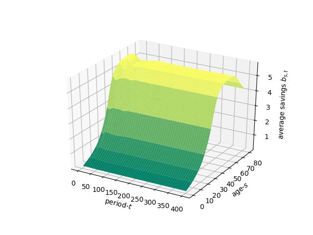
Contents

1 Introduction                                                                                                                5

2 Model structure                                                                                                             7
  2.1 Households . . . . . . . . . . . . . . . . . . . .     .   .   .   .   .   .   .   .   .   .   .   .   .   .   .   .    7
  2.2 Firms . . . . . . . . . . . . . . . . . . . . . . .    .   .   .   .   .   .   .   .   .   .   .   .   .   .   .   .   12
  2.3 Government — Household Taxes and Transfers             .   .   .   .   .   .   .   .   .   .   .   .   .   .   .   .   14
  2.4 Market Clearing . . . . . . . . . . . . . . . . . .    .   .   .   .   .   .   .   .   .   .   .   .   .   .   .   .   20
  2.5 Stationarisation . . . . . . . . . . . . . . . . . .   .   .   .   .   .   .   .   .   .   .   .   .   .   .   .   .   22

3 Calibration                                                                                                                25
  3.1 Demographics . . . . . . . . . . . . . . . . . . . . . . . .               .   .   .   .   .   .   .   .   .   .   .   25
  3.2 Lifetime Earnings Profiles . . . . . . . . . . . . . . . . .               .   .   .   .   .   .   .   .   .   .   .   33
  3.3 Calibration of Preference Parameters . . . . . . . . . . .                 .   .   .   .   .   .   .   .   .   .   .   35
  3.4 Calibration of Tax Functions with Microsimulation Data                     .   .   .   .   .   .   .   .   .   .   .   43

4 Concluding Remarks                                                                                                         48

Bibliography                                                                                                                 50

Appendices                                                                                                                   52

A Exogenous Inputs and Endogenous Output                                                                                     52
  A.1 Exogenous Parameters . . . . . . . . . . . . . . . . . . . . . . . . . . . . . .                                       52
  A.2 Endogenous Variables . . . . . . . . . . . . . . . . . . . . . . . . . . . . . . .                                     52

B Equilibrium Definitions and Solution Methods                                                                               52
  B.1 Stationary Steady-state Equilibrium . . . . . . . . . . . . . . . . . . . . . . .                                      52
  B.2 Stationary Non Steady-state Equilibrium . . . . . . . . . . . . . . . . . . . .                                        59

                                              4
1     Introduction
In this paper we present EDGE-M3, an overlapping generations (OLG) model for the EU coun-
tries.1 We discuss the model structure in detail, presenting all the equations of the model,
and take the example of Italy to illustrate its calibration.

    The most notable characteristic that differentiates an overlapping generations model from
other dynamic general equilibrium models is its more realistic representation of the finite life-
times of individuals and the cross-sectional age heterogeneity that exists in the economy. One
can make a strong case that age heterogeneity and income heterogeneity are two of the main
sources of diversity that explain much of the behaviour in which analysts and policy-makers
are interested, for instance when studying the differential effects of tax policy burdening
different categories of taxpayers. The model not only provides a steady-state solution, but
also simulates the transition of the economy from the initial state to the steady-state, which
provides the analyst with useful insight about the timing of economic responses to a policy
reform.

    EDGE-M3 is a general equilibrium model, which implies that the behaviour of households
and firms can cause macroeconomic variables and prices to adjust. EDGE-M3 is dynamic, in
the sense that households in the model make consumption, savings, and labour supply de-
cisions based on expectations over their entire lifetime, not just the current period. These
choices, in turn, dynamically affect the aggregate stock of capital thus affecting future pro-
duction. The model features overlapping generations of households endowed with different
levels of productivity (which we also refer to as “ability types” in the text), meaning that
within each simulated period, households of different age and income coexist. Each house-
hold in the model decides how much to participate to the labour force and how to allocate
earned income between consumption and savings, knowing that any residual wealth at the
end of its lifetime will be bequeathed to its descendants. Households optimise over their
lifetime, based on their expectations on labour earnings they can obtain (which in turns
also depends on their ability type) and interest rates on savings.2 Taxation affects net
wages, interest rates and the price of goods, thus it also influences how households and firms
behave. The only uncertainty faced by households in the model is due to their mortality risk.

   On the production side, one representative perfectly competitive firm maximises static
profits generated from the production of a single good by choosing capital and labour
demand. Production technology is described by the Cobb-Douglas function. Exogenous
productivity growth in the form of labour augmenting technological change is assumed.
EDGE-M3 can be optionally run assuming a closed economy or a partially open economy.

   The government collects taxes and distributes transfers to the households. In the current
version of the model we distinguish labour income tax, payroll tax, capital income taxes
(on savings and pension income), and consumption taxes (VAT and excises). The govern-
   1
     The model’s design was largely inspired by OG-USA , an open-source model for the US economy as
described in Evans and DeBacker (2019).
   2
     Households are represented by households’ heads, i.e. the person with the highest income in a household.

                                                     5
ment grants a general transfer to households that is composed of pension transfers and other
transfers. There are two options for the government closure in EDGE-M3 : by means of the
consumption tax or by means of the other than pension transfers. Since EDGE-M3 is a general
equilibrium model, all markets must clear. There are a capital market, a labour market and
a goods market in the model. The current version of the model is deterministic, i.e. there
are no aggregate shocks.

    In terms of calibration, the EDGE-M3 family of overlapping generations models makes use
of both macroeconomic and, most importantly, microeconomic data. In this way, the un-
derlying characteristics of the heterogeneous individuals are captured in the macro model.
For example, the parameters affecting the disutility of labour supply are calibrated using
data on hours worked and the EUROMOD microsimulation model. We match labour elasticities
estimated using the micro-data to the more aggregated individual agents of our OLG model
to produce a labour supply curve. To obtain realistic consumption profiles, our model’s
parameters have been calibrated to closely reproduce the actual wealth and bequests distri-
butions in a specific country.

    A feature of the model which is of particular interest is the richness of its income tax
functions. In order to model taxes and following DeBacker et al. (2019), we equip the
EDGE-M3 model with non-linear income tax functions estimated using the output from the
EUROMOD microsimulation model. We assume that tax rates on labour income and capital
income are bivariate non-linear functions of labour income and capital income. Thanks to
this highly disaggregated approach, important characteristics of the complex tax system are
automatically accounted for by means of the parameterised tax functions that enter the
macro model.3
Furthermore, we separately estimate a social insurance contribution function using the un-
derlying microeconomic data. We consider mandatory contributions to pension schemes
separately from income taxation due to their nature of forced savings. This approach also
enables more controlled policy experiments, for instance in order to examine tax reforms
under a ceteris paribus condition with respect to the pension system, and vice versa.

   In sum, the richness of the EDGE-M3 model makes it highly suitable for a joint analysis of
the individual savings and labour responses, the macroeconomic effects as well as the inter-
and intragenerational impact of pressing policy questions including, but not limited to:

    • demographic change, since EDGE-M3 includes yearly country-specific demographic pro-
      jections from Eurostat for fertility rates, mortality rates and immigration rates;

    • reforms of social insurance contributions or labour and capital income taxes, such as
      shifts from labour to capital;
   3
     The estimation of the income tax functions is detailed in Section 3.4. In d’Andria et al. (2019), we illus-
trate the methodology of including non-linear income tax functions into the EDGE-M3 model by first examining
the effect of a reduction in marginal personal income tax rates in Italy with the EUROMOD microsimulation
model and then translating the microsimulation results into a shock for the overlapping generations model.

                                                       6
• distributional concerns, including changes to the progressivity of the tax system, where
      results may critically hinge on the behaviour of the top share of earners;

    • pension system reforms and their distributional impact, e.g. increasing the retirement
      age, changing the pension contribution rate or switching from one pension system to
      another one.

   The EDGE-M3 is currently being extended to analyse European pension systems, namely
the defined benefit, the defined contribution and the point system.

    The paper is structured as follows. In Section 2 we discuss the model structure presenting
all the equations and assumptions, detailing the functional forms used. Section 3 presents
the calibration of the model using both macroeconomic and microeconomic data. Section 4
finally offers some concluding remarks.

2       Model structure
In this section, we present in detail the EDGE-M3 model structure.

2.1     Households
The household is, in many respects, the most important economic agent in the EDGE-M3 model.
We model households in EDGE-M3 rather than individuals, because we want to abstract from
the concepts of gender, marital status, and number of children.4 Therefore, it is appropriate
to use the household as the most granular unit of account.

2.1.1    Budget Constraint
We described the derivation and dynamics of the population distribution in Section 3.1. A
measure ω1,t of households is born each period, become economically relevant at age s = E+1
if they survive to that age, and live for up to E + S periods (S economically active periods),
with the population of age-s individuals in period t being ωs,t . Let the age of a household
be indexed by s = {1, 2, ...E + S}.
    At birth, each household age s = 1 is randomly assigned one of J ability groups,    P indexed
by j. Let λj represent the fraction of individuals in each ability group, such that j λj = 1.
Note that this implies that the distribution across ability types in each age is given by
λ = [λ1 , λ2 , ...λJ ]. Once a household member is born and assigned to an ability type,
he remains that ability type for his entire lifetime. Thus, it is the deterministic ability
heterogeneity as an agent cannot change his ability type (for more details see Section 3.2).
Let ej,s > 0 be a matrix of ability-levels such that an individual of ability type j will have
lifetime abilities of [ej,1 , ej,2 , ...ej,E+S ]. The budget constraint for the age-s household in
    4
     The curse of dimensionality forces us to focus on those household characteristics – age and ability – most
relevant for the analyses considered.

                                                      7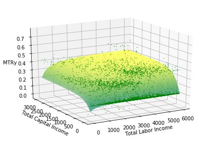
lifetime income group j at time t is the following,

            c
                                                                        BQt               T Rt      I        P
cj,s,t 1 + τs,t   + bj,s+1,t+1 = (1 + rt )bj,s,t + wt ej,s nj,s,t + ζj,s         + ηj,s,t         − Tj,s,t − Tj,s,t
                                                                         λj ωs,t          λj ωs,t
                                ∀j, t and s ≥ E + 1 where bj,E+1,t = 0 ∀j, t
                                                                                                               (1)
                                  c
where cj,s,t is consumption, τs,t     is consumption tax rate, bj,s+1,t+1 is savings for the next
period, rt is the interest rate (return on savings), bj,s,t is current period wealth (savings from
last period), wt is the wage, and nj,s,t is labour supply.
    The next term on the right-hand-side of the budget constraint (1) represents the portion
of total bequests BQt that go to the age-s, income-group-j household. Let ζj,s be the
fraction
PE+S P     of total bequests BQt that go to the age-s, income-group-j household, such that
             J
   s=E+1     j=1 ζj,s = 1. We must divide that amount by the population of (j, s) households
λj ωs,t . Section 3.3.2 details how to calibrate the ζj,s values from consumer finance data.
    The penultimate term on the right-hand-side of the budget constraint (1) represents the
portion of total transfers T Rt that go to the age-s, income-group-j household. Let ηj,s,t be
the
PE+Sfraction
           PJ of total transfers T Rt that go to the age-s, income-group-j household, such that
   s=E+1     j=1 ηj,s,t = 1. We must divide that amount by the population of (j, s) households
λj ωs,t . Section 2.3.3 details how transfers are distributed among households.
    The last two terms on the right-hand-side of the budget constraint (1) represent income
                                I                      P
taxes paid by households, Tj,s,t   , and payroll tax, Tj,s,t .

2.1.2       Elliptical Disutility of Labour Supply
In EDGE-M3 , the period utility function of each household is a function of consumption cj,s,t ,
savings bj,s+1,t+1 , and labour supply nj,s,t .5 We detail this utility function, its justification,
and functional form in Section 2.1.3. With endogenous labour supply nj,s,t , we must specify
how labour enters an agent’s utility function and what are the constraints. Assume that
each household is endowed with a measure of time ˜l each period that it can choose to spend
as either labour nj,s,t ∈ [0, ˜l] or leisure lj,s,t ∈ [0, ˜l].

                                           nj,s,t + lj,s,t = ˜l ∀s, t                                          (2)

    The functional form for the utility of leisure or the disutility of labour supply has im-
portant implications for the computational tractability of the model. One difference of the
household’s labour supply decision nj,s,t from the consumption decision cj,s,t is that the con-
sumption decision only has a lower bound cj,s,t ≥ 0 whereas the labour supply decision has
both upper and lower bounds nj,s,t ∈ [0, ˜l]. Evans and Phillips (2018) show that many of
the traditional functional forms for the disutility of labour—Cobb-Douglas, constant Frisch
elasticity, constant relative risk aversion (CRRA)—do not have Inada conditions on both
the upper and lower bounds of labour supply. To solve these in a heterogeneous agent model
would require occasionally binding constraints, which is a notoriously difficult computational
problem.
   5
       Savings enters the period utility function to provide a “warm glow” bequest motive.

                                                        8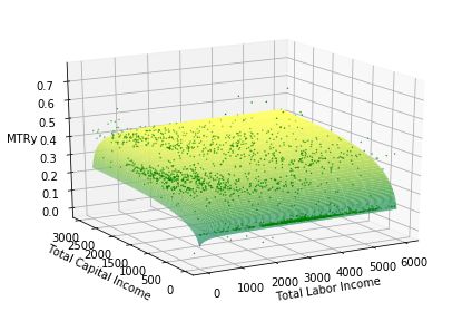
Figure 1: Comparison of CFE marginal disutility
                                of leisure θ = 0.9 to fitted elliptical util-
                                ity

    Evans and Phillips (2018) propose using an equation for an ellipse to match the disutility
of labour supply to whatever traditional functional form one wants. Our preferred specifi-
cation in EDGE-M3 is to fit an elliptical disutility of labour supply function to approximate
a linearly separable constant Frisch elasticity (CFE) functional form. Let v(n) be a general
disutility of labour function. A CFE disutility of labour function is the following,
                                                         1
                                                n1+ θ
                                         v(n) ≡        ,     θ>0                                       (3)
                                                1 + 1θ
where θ > 0 represents the Frisch elasticity of labour supply. The elliptical disutility of
labour supply functional form is the following,
                                            υ  υ1
                                              n
                            v(n) = −b 1 −             , b, υ > 0                        (4)
                                              ˜l
where b > 0 is a scale parameter and υ > 0 is a curvature parameter. This functional form
satisfies both v 0 (n) > 0 and v 00 (n) > 0 for all n ∈ (0, 1). Further, it has Inada conditions at
both the upper and lower bounds of labour supply limn→0 v 0 (n) = 0 and limn→l̃ v 0 (n) = −∞.
    Because it is the marginal disutility of labour supply that matters for household decision
making, we want to choose the parameters of the elliptical disutility of labour supply function
(b, υ) so that the elliptical marginal utilities match the marginal utilities of the CFE disutility
of labour supply. Figure 1 shows the fit of marginal utilities for a Frisch elasticity of θ = 0.9
and a total time endowment of ˜l = 1.0. The estimated elliptical utility parameters in this
case are b = 0.527 and υ = 1.497.6
  6
      Peterman (2016) shows that in a macro-model that has only an intensive margin of labour supply and no

                                                     9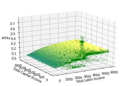
2.1.3      Optimality Conditions
Households choose lifetime consumption {cj,s,t+s−1 }Ss=1 , labour supply {nj,s,t+s−1 }Ss=1 , and
savings {bj,s+1,t+s }Ss=1 to maximise lifetime utility, subject to the budget constraints and non
negativity constraints. The household period utility function is the following.
                                                                                                 υ  υ1
                                               (cj,s,t )1−σ − 1

                                                                      gy t(1−σ) n         nj,s,t
          u(cj,s,t , nj,s,t , bj,s+1,t+1 ) ≡                      +e           χs b 1 −                   +
                                                     1−σ                                    ˜l
                                                                                                            (5)
                                                                1−σ
                                                 (b j,s+1,t+1 )     − 1
                                          χbj ρs                            ∀j, t and E + 1 ≤ s ≤ E + S
                                                         1−σ
The period utility function (5) is linearly separable in cj,s,t , nj,s,t , and bj,s+1,t+1 . The first
term is a constant relative risk aversion (CRRA) utility of consumption. The second term
is the elliptical disutility of labour described in Section 2.1.2. The constant χns adjusts the
disutility of labour supply relative to consumption and can vary by age s, which is helpful
for calibrating the model to match labour market moments. See Section 3.4 for a discussion
of the calibration.
     It is necessary to multiply the disutility of labour in (5) by egy (1−σ) because labour supply
nj,s,t is stationary, but both consumption cj,s,t and savings bj,s+1,t+1 are growing at the rate
of technological progress (see Section 2.5). The egy (1−σ) term keeps the relative utility values
of consumption, labour supply, and savings in the same units.
     The final term in the period utility function (5) is the “warm glow” bequest motive. It is
a CRRA utility of savings, discounted by the mortality rate ρs .7 Intuitively, it represents the
utility a household gets in the event that they don’t live to the next period with probability
ρs . It is a utility of savings beyond its usual benefit of allowing for more consumption in
the next period. This utility of bequests also has constant χbj which adjusts the utility of
bequests relative to consumption and can vary by lifetime income group j. This is helpful
for calibrating the model to match wealth distribution moments. See Section 3.4 for a
discussion of the calibration. Note that any bequest before age E + S is unintentional as
it was bequeathed due an event of death that was uncertain. Intentional bequests are all
bequests given in the final period of life in which death is certain bj,E+S+1,t .
     The household lifetime optimisation problem is to choose consumption cj,s,t , labour supply
nj,s,t , and savings bj,s+1,t+1 in every period of life to maximise expected discounted lifetime
utility, subject to budget constraints and upper-bound and lower-bound constraints.
                                           S
                                           X
                                                 β s−1 ΠE+s

                max                                     u=E+1 (1 − ρu )  u(cj,s,t+s−1 , nj,s,t+s−1 , bj,s+1,t+s )   (6)
{(cj,s,t ),(nj,s,t ),(bj,s+1,t+1 )}E+S
                                   s=E+1   s=1

                       c
                                                                                   BQt               T Rt      I        P
      s.t. cj,s,t 1 + τs,t   + bj,s+1,t+1 = (1 + rt )bj,s,t + wt ej,s nj,s,t + ζj,s         + ηj,s,t         − Tj,s,t − Tj,s,t
                                                                                    λj ωs,t          λj ωs,t
                                                                                                              (1)
         and cj,s,t ≥ 0, nj,s,t ∈ [0, ˜l], and bj,E+1,t = 0 ∀j, t, and E + 1 ≤ s ≤ E + S
extensive margin and represents a broad composition of individuals supplying labour—such as EDGE-M3 —
a Frisch elasticity of around 0.9 is probably appropriate. He tests the implied macro elasticity when the
assumed micro elasticities are small on the intensive margin but only macro aggregates—which include both
extensive and intensive margin agents—are observed.
   7
     See Section 3.1.2 of Section 3.1 for a detailed discussion of mortality rates in EDGE-M3 .

                                                                 10
The non-negativity constraint on consumption does not bind in equilibrium because of the
Inada condition limc→0 u1 (c, n, b0 ) = ∞, which implies consumption is always strictly positive
in equilibrium cj,s,t > 0 for all j, s, and t. The warm glow bequest motive in (5) also has
an Inada condition for savings at zero, so bj,s,t > 0 for all j, s, and t. This is an implicit
borrowing constraint.8 And finally, as discussed in Section 2.1.2, the elliptical disutility
of labour supply functional form in (5) imposes Inada conditions on both the upper and
lower bounds of labour supply such that labour supply is strictly interior in equilibrium
nj,s,t ∈ (0, ˜l) for all j, s, and t.
The household maximisation problem can be further reduced by substituting in the house-
hold budget constraint, which binds with equality. This simplifies the household’s problem
to choosing labour supply nj,s,t and savings bj,s+1,t+1 every period to maximise lifetime dis-
counted expected utility. The 2S first order conditions for every type-j household that
characterise the its S optimal labour supply decisions and S optimal savings decisions are
the following.
I P
! υ−1 " υ # 1−υ
υ
∂Tj,s,t ∂Tj,s,t
1 gy (1−σ) n b nj,s,t nj,s,t
wt ej,s − − (cj,s,t )−σ =e χs 1−
∂nj,s,t ∂nj,s,t c
1 + τs,t ˜l ˜l ˜l
∀j, t, and E + 1 ≤ s ≤ E + S
(7)
I
∂Tj,s+1,t+1
−σ 1 −gy σ
χbj ρs (bj,s+1,t+1 )−σ (cj,s+1,t+1 )−σ
(cj,s,t ) c
=e + β 1 − ρs 1 + rt+1 −
1 + τs,t ∂bj,s+1,t+1
1
c
1 + τs+1,t+1
∀j, t, and E + 1 ≤ s ≤ E + S − 1
(8)
(cj,E+S,t )−σ = χbj (bj,E+S+1,t+1 )−σ ∀j, t and s = E + S (9)
∂Ts,t
where the marginal income tax rate with respect to labour supply ∂nj,s,t
is described in
P
∂Tj,s,t
equation (28). ∂nj,s,t
is the marginal rate of payroll tax with respect to labour supply.
2.1.4 Expectations
To conclude the household’s problem, we must make an assumption about how the age-s
household can forecast the time path of interest rates, wages, and total bequests {ru , wu , BQu }t+S−s
u=t
over his remaining lifetime. As shown in Appendices B.1 and B.2, the equilibrium interest
8
It is important to note that savings also has an implicit upper bound bj,s,t ≤ k above which consumption
would be negative in current period. However, this upper bound on savings is taken care of by the Inada
condition on consumption.
11rate rt , wage wt , and total bequests BQt will be functions of the state vector Γt , which turns
out to be the entire distribution of savings in period t.
Define Γt as the distribution of household savings across households at time t.
E+S
Γt ≡ bj,s,t s=E+2
∀j, t (10)
Let general beliefs about the future distribution of capital in period t + u be characterised
by the operator Ω(·) such that:
Γet+u = Ωu (Γt ) ∀t, u≥1 (11)
where the e superscript signifies that Γet+u is the expected distribution of wealth at time t + u
based on general beliefs Ω(·) that are not constrained to be correct.9
2.2 Firms
The production side of the EDGE-M3 model is populated by a unit measure of identical per-
fectly competitive firms that rent capital Kt and hire labour Lt to produce output Yt .
2.2.1 Production Function
Firms produce output Yt using inputs of capital Kt and labour Lt according to the Cobb-
Douglas production function:
Yt = Zt (Kt )γ (egy t Lt )1−γ (12)
where Zt is an exogenous scale parameter (total factor productivity) that can be time depen-
dent and γ represents the capital share of income. We have included constant productivity
growth gy as the rate of labour augmenting technological progress.
The Cobb-Douglas production function is a special case of the general constant elasticity
(CES) of substitution production function,
ε
ε−1
1 ε−1 1 ε−1
g t
Yt = F (Kt , Lt ) ≡ Zt (γ) ε (Kt ) ε + (1 − γ) ε (e y Lt ) ε ∀t (13)
for ε = 1.
2.2.2 Optimality Conditions
The profit function of the representative firm is the following.
P Rt = F (Kt , Lt ) − wt Lt − rt + δ Kt ∀t (14)
Gross income for the firms is given by the production function F (K, L) because we have
normalised the price of the consumption good to 1. Labour costs to the firm are wt Lt , and
capital costs are (rt + δ)Kt . The per-period economic depreciation rate is given by δ.
9
In Appendix B.2 we will assume that beliefs are correct (rational expectations) for the non-steady-state
equilibrium in Definition 2.
12Taking the derivative of the profit function (14) with respect to labour Lt and setting it
equal to zero and taking the derivative of the profit function with respect to capital Kt and
setting it equal to zero, respectively, characterises the optimal labour and capital demands.
Yt
wt = (1 − γ) ∀t (15)
Lt
Yt
rt = γ −δ ∀t (16)
Kt
2.2.3 Small Open Economy
In addition to a closed economy version, the EDGE-M3 model also accommodates small and
partially open economies. In the small open economy version of the EDGE-M3 model, the
country faces an exogenous world interest rate, rt∗ that determines the amount of savings
and investment. If the supply of savings from households does not meet the demand for
private capital and private borrowing, foreign capital will flow in to make excess demand
zero at the world interest rate.
Let the total capital stock be given by the quantity of domestically supplied capital and
foreign supplied capital, i.e., Kt = Ktd + Ktf . Then foreign capital is given by:
Ktf = Ktdemand − (Bt − Dt ) (17)
where Bt is aggregate household savings and Dt is government borrowing. Capital demand
is determined from the firm’s first order condition (16) for its choice of capital, given rt∗ .
2.2.4 Partially Open Economy
In the partially open economy version of EDGE-M3 , the openness of the economy is mod-
elled through two parameters that capture the extent of foreign lending to the domestic
government and the amount of foreign lending of private capital to firms.
First, this version of the model accommodates foreign held public debt. In particular,
the parameter ζD gives the share of new debt issues that are purchased by foreigners. The
law of motion for foreign-held debt is therefore given by:
f
Dt+1 = Dtf + ζD (Dt+1 − Dt ) (18)
Domestic debt holdings then are determined as the remaining debt holdings needed to meet
government demand for debt:
Dtd = Dt − Dtf (19)
Second, whereas total capital demand still follows from the exogenous world interest
rate, the parameters ζK helps to determine the share of domestic capital held by foreigners.
In particular, let Ktopen be the amount of capital that would need to flow into the country
to meet firm demand for capital at the exogenous world interest rate from the small open
economy specification, net of what domestic households can supply:
Ktopen = Ktdemand − (Bt − Dt ) (20)
13where, Ktdemand is total capital demand by domestic firms at rt∗ , Bt are total asset holdings
of domestic households, and Dt are holdings of government debt by domestic households.
Importantly, total asset holdings from households result from solving the household’s op-
timisation problem at the endogenous home country interest rate. Note that there thus is
a disconnect between the interest rates that determine firm capital demand and domestic
household savings and the interest rate used to determine Ktdemand . This assumption is useful
in that it nests the small open economy case into the partial open economy model. However,
it does leave out the realistic responses of foreign capital supply to differentials in the home
country interest rate and the world interest rate.
Next, given Ktopen , ζK can be used to determine the foreign capital held by foreigners in
the small open economy specification:
Ktf = ζK Ktopen (21)
Given the two equations above, we can find the total supply of capital as:
Ktsupply = Ktd + Ktf
= Bt − Dtd + ζK Ktopen (22)
2.3 Government — Household Taxes and Transfers
The government is not an optimising agent in EDGE-M3 . The government levies taxes on
households and provides transfers to households. The government sector influences house-
holds through three terms in the household budget constraint given by formula (1): govern-
I
ment transfers T Rt , total income tax liability function Ts,t , which can be decomposed into
10
the effective income tax rate times total income (see equation (25)), and the consumption
I
tax rate. In this section, we detail the household tax component of government activity Ts,t
in EDGE-M3 , along with our method of incorporating detailed microsimulation data into a
dynamic general equilibrium model. Finally, this section discusses the government’s resulting
budget constraint.
2.3.1 Income Taxation
Incorporating realistic tax and incentive detail into a general equilibrium model is notoriously
difficult for two reasons. First, it is impossible in a dynamic general equilibrium (DGE)
model to capture all of the dimensions of heterogeneity on which the real-world tax rate
depends. For example, a household’s tax liability in reality depends on filing status, number
of dependants, many types of income, and some characteristics correlated with age. A
good heterogeneous agent DGE model tries to capture the most important dimensions of
heterogeneity, and necessarily neglects the other dimensions.
The second difficulty in modelling realistic tax and incentive detail is the need for good
microeconomic data on the individuals who make up the economy from which to simulate
behavioural responses and corresponding tax liabilities and tax rates.
10
In this paper effective tax rate refers to the average effective tax rate.
14EDGE-M3 follows the method of DeBacker et al. (2019) of generating detailed income tax
data on effective tax rates and marginal tax rates for a sample of tax filers along with their
respective income and demographic characteristics and then using that data to estimate
parametric tax functions that can be incorporated into EDGE-M3 .
Effective and Marginal Tax Rates Before going into more detail regarding how we
handle these two difficulties in EDGE-M3 , we need to define some functions and make some
notation. For notational simplicity, we will use the variable x to summarise labour income,
and we will use the variable y to summarise capital income.
xj,s,t ≡ wt ej,s nj,s,t ∀j, t and E + 1 ≤ s ≤ E + S (23)
yj,s,t ≡ rt bj,s,t ∀j, t and E + 1 ≤ s ≤ E + S (24)
Part of total tax liability Tj,s,t from the household budget constraint 1 is income tax
I
liability Tj,s,t that can be expressed as an effective tax rate multiplied by total income.
I etr
Tj,s,t = τs,t (xj,s,t , yj,s,t ) (xj,s,t + yj,s,t ) (25)
Rearranging equation (25) gives the definition of an effective tax rate (ET R) as total
income tax liability divided by the unadjusted gross income, or rather, total income tax
liability as a percent of unadjusted gross income. A marginal income tax rate (M T R) is
defined as the change in total tax liability from a small change income. In EDGE-M3 , we
differentiate between the marginal tax rate on labour income (M T Rx) and the marginal tax
rate on labour income (M T Ry).
I I
∂Tj,s,t ∂Tj,s,t
τ mtrx ≡ = ∀j, t and E + 1 ≤ s ≤ E + S (26)
∂wt ej,s nj,s,t ∂xj,s,t
I I
mtry
∂Tj,s,t ∂Tj,s,t
τ ≡ = ∀j, t and E + 1 ≤ s ≤ E + S (27)
∂rt bj,s,t ∂yj,s,t
As we show in Section 2.1.3, the derivative of total income tax liability with respect to
I
∂Ts,t
labour supply ∂nj,s,t and the derivative of total income tax liability next period with respect
∂T I
s+1,t+1
to savings ∂bj,s+1,t+1 show up in the household Euler equations for labour supply given in
equation (7) and savings given in equation (8), respectively. It is valuable to be able to
express those marginal tax rates, for which we have no data, as marginal tax rates for which
we do have data. The following two expressions show how the marginal tax rates of labour
supply can be expressed as the marginal tax rate on labour income times the household-
specific wage and how the marginal tax rate of savings can be expressed as the marginal tax
rate of capital income times the interest rate.
I I I
∂Tj,s,t ∂Tj,s,t ∂wt ej,s nj,s,t ∂Tj,s,t mtrx
= = wt ej,s = τs,t wt ej,s (28)
∂nj,s,t ∂wt ej,s nj,s,t ∂nj,s,t ∂wt ej,s nj,s,t
I I I
∂Tj,s,t ∂Tj,s,t ∂rt bj,s,t ∂Tj,s,t mtry
= = rt = τs,t rt (29)
∂bj,s,t ∂rt bj,s,t ∂bj,s,t ∂rt bj,s,t
15Fitting Tax Functions In looking at the 3D scatter plots of ET R, M T Rx, and M T Ry
in Figure 2, it is clear that all of these rates exhibit negative exponential or logistic shape.
This empirical regularity allows us to make an important and non-restrictive assumption.
We can fit parametric income tax rate functions to these data that are constrained to be
monotonically increasing in labour income and capital income. This assumption of mono-
tonicity is computationally important as it preserves a convex budget set for each household,
which is important for being able to solve many household lifetime problems over a large
number of periods.
Figure 2: Scatter plot of ETR, MTRx, MTRy, and histogram as functions of
labour income and capital income from microsimulation model, year
2015
(a) Effective tax rates ET R (b) Marginal tax rates on labour income
M T Rx
(c) Marginal tax rates on capital income (d) Histogram
M T Ry
EDGE-M3 follows the approach of DeBacker et al. (2019) in using the functional form
expressed by equation (30) to estimate income tax functions for each time period t. The
estimation can be performed separately for each age s = E + 1, E + 2, ..., E + S, or divid-
ing observations into age bins and then estimating functions for each bin. The option to
have age-dependent estimations comes useful when the data displays heterogeneous compo-
sitions in incomes that vary with age. As different income items are often treated differently
16tax-wise, for example in the case of property or pension income, having age-specific tax
functions allows to indirectly capture such heterogeneity thus providing better estimates.
Age-dependent tax functions and the size in years of each age bin for which the estimation
is performed can be changed via parameters, in order to be able to deal with the specific
micro data used for this purpose.
Equation (30) is written as a generic tax rate, but we use this same functional form for
ET R0 s, M T Rx0 s, and M T Ry 0 s.
τ (x, y) = [τ (x) + shif tx ]φ [τ (y) + shif ty ]1−φ + shif t
Ax2 + Bx
where τ (x) ≡ (maxx − minx ) + minx
Ax2 + Bx + 1
Cy 2 + Dy
(30)
and τ (y) ≡ (maxy − miny ) + miny
Cy 2 + Dy + 1
where A, B, C, D, maxx , maxy , shif tx , shif ty > 0 and φ ∈ [0, 1]
and maxx > minx and maxy > miny
The parameters values will, in general, differ across the different functions (effective and
marginal rate functions) and by age, s, and tax year, t. We drop the subscripts for age and
year from the above exposition for clarity.
By assuming each tax function takes the same form, we are breaking the analytical link
between the the effective tax rate function and the marginal rate functions. In particular, one
could assume an effective tax rate function and then use the analytical derivative of that to
find the marginal tax rate function. However, we have found it useful to separately estimate
the marginal and average rate functions. One reason is that we want the tax functions to be
able to capture policy changes that have differential effects on marginal and average rates.
For example, a change in the standard deduction for tax payers would have a direct effect on
their average tax rates. But it will have secondary effect on marginal rates as well, as some
filers will find themselves in different tax brackets after the policy change. These are smaller
and second order effects. When tax functions are fit to the new policy, in this case a lower
standard deduction, we want them to be able to represent this differential impact on the
marginal and average tax rates. The second reason is related to the first. As the additional
flexibility allows us to model specific aspects of tax policy more closely, it also allows us to
better fit the parameterised tax functions to the data.
The key building blocks of the functional form equation (30) are the τ (x) and τ (y)
2 +Bx
univariate functions. The ratio of polynomials in the τ (x) function with positive AxAx2 +Bx+1
coefficients A, B > 0 and positive support for labour income x > 0 creates a negative-
exponential-shaped function that is bounded between 0 and 1, and the curvature is governed
by the ratio of quadratic polynomials. The multiplicative scalar term (maxx − minx ) on the
ratio of polynomials and the addition of minx at the end of τ (x) expands the range of the
univariate negative-exponential-shaped function to τ (x) ∈ [minx , maxx ]. The τ (y) function
is an analogous univariate negative-exponential-shaped function in capital income y, such
that τ (y) ∈ [miny , maxy ].
17The respective shif tx and shif ty parameters in equation (30) are analogous to the addi-
tive constants in a Stone-Geary utility function. These constants ensure that the two sums
τ (x) + shif tx and τ (yx) + shif ty are both strictly positive. They allow for negative tax
rates in the τ (.) functions despite the requirement that the arguments inside the brack-
ets be strictly positive. The general shift parameter outside of the Cobb-Douglas brackets
can then shift the tax rate function so that it can accommodate negative tax rates. The
Cobb-Douglas share parameter φ ∈ [0, 1] controls the shape of the function between the two
univariate functions τ (x) and τ (y).
This functional form for tax rates delivers flexible parametric functions that can fit the
tax rate data shown in Figure 2 as well as a wide variety of policy reforms. Further, these
functional forms are monotonically increasing in both labour income x and capital income
y. This characteristic of monotonicity in x and y is essential for guaranteeing convex budget
sets and thus uniqueness of solutions to the household Euler equations. The assumption
of monotonicity does not appear to be a strong one when viewing the tax rate data shown
in Figure 2. While it does limit the potential tax systems to which one could apply our
methodology, tax policies that do not satisfy this assumption would result in non-convex
budget sets and thus require non-standard DGE model solutions methods and would not
guarantee a unique equilibrium. The 12 parameters of our tax rate functional form from
equation (30) are summarised in Table 1.
Table 1: Description of tax rate function τ (x, y) parameters
Symbol Description
A Coefficient on squared labour income term x2 in τ (x)
B Coefficient on labour income term x in τ (x)
C Coefficient on squared capital income term y 2 in τ (y)
D Coefficient on capital income term y in τ (y)
maxx Maximum tax rate on labour income x given y = 0
minx Minimum tax rate on labour income x given y = 0
maxy Maximum tax rate on capital income y given x = 0
miny Minimum tax rate on capital income y given x = 0
shif tx shif ter > |minx | ensures that τ (x) + shif tx > 0 despite potentially
negative values for τ (x)
shif ty shif ter > |miny | ensures that τ (y) + shif ty > 0 despite potentially
negative values for τ (y)
shif t shifter (can be negative) allows for support of τ (x, y) to include
negative tax rates
φ Cobb-Douglas share parameter between 0 and 1
Source: DeBacker et al. (2019)
Factor Transforming Income Units The income tax functions τ etr , τ mtrx , τ mtry are
estimated based on current Italian tax filer reported incomes in Euros. However, the con-
sumption units of the EDGE-M3 model are not in the same units as the real-world Italian
18income data. For this reason, we have to transform the income by a f actor so that it is in
the same units as the income data on which the tax functions were estimated.
The tax rate functions are each functions of capital income and labour income τ (x, y).
In order to make the tax functions return accurate tax rates associated with the correct
levels of income, we multiply the model income xm and y m by a f actor. The f actor trans-
lates model units into the data units (Euros). Thus, we need to multiply model taxable
income by a factor to get the same units as the real-world Italian income in tax data
τ (f actor × xm , f actor × y m ). We define the f actor such that average steady-state house-
hold total income in the model times the f actor equals the Italian tax data average total
income.
" E+S J
#
X X
f actor λj ωs (wej,s nj,s + rbj,s ) = average household income in tax data
s=E+1 j=1
(31)
We do not know the steady-state wage, interest rate, household labour supply, and sav-
ings ex ante. So the income f actor is an endogenous variable in the steady-state equilibrium
computational solution. We hold the factor constant throughout the non-steady-state equi-
librium solution.
2.3.2 Consumption Tax
Consumption tax is the average tax paid on all goods and services, including both value-
added tax and excise duties. in EDGE-M3 consumption tax rates are differentiated by age.
In Section 3.4.3 we discuss how the consumption tax rates are calibrated in EDGE-M3 using
micro data.
2.3.3 Household Transfers
Total transfers to households by the government in a given period t is T Rt . The percent
of those transfers given to all households of age s and lifetime income group j is ηj,s such
that E+S
P PJ
s=E+1 j=1 ηj,s,t = 1. In the current calibration EDGE-M3 has the transfer distribution
function set to distribute transfers uniformly among the population.
λj ωs,t
ηj,s,t = ∀j, t and E + 1 ≤ s ≤ E + S (32)
Ñt
However, this distribution function ηj,s,t could also be modified to more accurately reflect
the way transfers are distributed in Italy.
2.3.4 Government Budget Constraint
Let the level of government debt in period t be given by Dt . The government budget
constraint requires that government revenues Revt from income and consumption taxes plus
the budget deficit (Dt+1 − Dt ) equal expenditures on interest of the debt and government
spending on transfer payments to households T Rt every period t.
19Dt+1 + Revt = (1 + rgov,t )Dt + T Rt ∀t (33)
Despite the model having no aggregate risk, it may be helpful to build in an interest rate
differential between the rate of return on private capital and the interest rate on government
debt. Doing so helps to add realism by including a risk premium. EDGE-M3 allows users to
set an exogenous wedge between these two rates:
rgov,t = (1 − τd,t )rt − µd (34)
The two parameters, τd,t and µd can be used to allow for a government interest rate (rgov,t )
that is a percentage hair cut from the market rate or a government interest rate with a
constant risk premium.
In the cases where there is a differential (τd,t or µd 6= 0), then we need to be careful to
specify how the household chooses government debt and private capital in its portfolio of
asset holdings. We make the assumption that under the exogenous interest rate wedge, the
household is indifferent between holding its assets as debt and private capital. This amounts
to an assumption that these two assets are perfect substitutes given the exogenous wedge in
interest rates. Given the indifference between government debt and private capital at these
two interest rates, we assume that the household holds debt and capital in the same ratio
that debt and capital are demanded by the government and private firms, respectively. The
interest rate on the household portfolio of asset is thus given by:
rgov,t Dt + rt Kt
rhh,t = (35)
Dt + Kt
2.4 Market Clearing
Three markets must clear in EDGE-M3 —the labour market, the capital market, and the
goods market. By Walras’ Law, we only need to use two of those market clearing conditions
because the third one is redundant. In the model, we choose to use the labour market
clearing condition and the capital market clearing condition. The (redundant) goods market
clearing condition—sometimes referred to as the resource constraint—is used as a check on
the solution method. We present all three market clearing conditions here.
We also characterise here the law of motion for total bequests BQt . Although it is not
technically a market clearing condition, one could think of the bequests’ law of motion as
the bequests’ market clearing condition.
2.4.1 Market Clearing Conditions
Labour market clearing (see equation (36) below) requires that aggregate labour demand Lt
measured in efficiency units equal the sum of household efficiency labour supplied ej,s nj,s,t .
E+S
X J
X
Lt = ωs,t λj ej,s nj,s,t ∀t (36)
s=E+1 j=1
20Capital market clearing (see (37)) requires that aggregate capital demand from firms Kt
equal the sum of capital savings and investment by households bj,s,t .
E+S+1
X X J
Kt = ωs−1,t−1 λj bj,s,t + is ωs,t−1 λj bj,s,t ∀t (37)
s=E+2 j=1
Aggregate consumption Ct is defined as the sum of all household consumptions, and
aggregate investment is defined by the resource constraint Yt = Ct + It as shown in equation
(38).
E+S+1
X X J
Yt = Ct + Kt+1 − is ωs,t λj bj,s,t+1 − (1 − δ)Kt ∀t
s=E+2 j=1
E+S J
(38)
X X
where Ct ≡ ωs,t λj cj,s,t
s=E+1 j=1
Note that the extra terms with the immigration rate is in the capital market clearing
equation (37) and the resource constraint (38) accounts for the assumption that age-s im-
migrants in period t bring with them (or take with them in the case of out-migration) the
same amount of capital as their domestic counterparts of the same age. Note also that the
term in parentheses with immigration rates is in the sum acts is equivalent to a net exports
term in the standard equation Y = C + I + G + N X. That is, if immigration rates are
positive, then immigrants are bringing capital into the country and the term in parentheses
has a negative sign in front of it. Negative exports are imports.
2.4.2 Total Bequests Law of Motion
Total bequests BQt are the collection of savings of household from the previous period who
died at the end of the period. These savings are augmented by the interest rate because they
are returned after being invested in the production process.
E+S+1 J
!
X X
BQt = (1 + rt ) ρs−1 λj ωs−1,t−1 bj,s,t ∀t (39)
s=E+2 j=1
Because the form of the period utility function in (5) ensures that bj,s,t > 0 for all j, s, and
t, total bequests will always be positive BQj,t > 0 for all j and t.
2.4.3 Total Transfers Law of Motion
Total transfers to households T Rt are the collection of all taxes paid by households, i.e.
I C
income taxes, Tj,s,t and consumption taxes, Tj,s,t .
E+S+1 J E+S+1 J
!
X X X X
I C
T Rt = λj ωs−1,t−1 Tj,s,t + λj ωs−1,t−1 Tj,s,t ∀t. (40)
s=E+2 j=1 s=E+2 j=1
212.5 Stationarisation
The previous sections derive all the equations necessary to solve for the steady-state and
non-steady-state equilibria of this model. However, because labour productivity is growing
at rate gy as can be seen in the firms’ production function (13) and the population is growing
at rate g̃n,t as defined in (58), the model is not stationary. Different endogenous variables of
the model are growing at different rates.
Table 2 lists the definitions of stationary versions of these endogenous variables. Variables
with a “ ˆ ” signify stationary variables. The first column of variables are growing at the
productivity growth rate gy . These variables are most closely associated with individual
variables. The second column of variables are growing at the population growth rate g̃n,t .
These variables are most closely associated with population values. The third column of
variables are growing at both the productivity growth rate gy and the population growth rate
g̃n,t . These variables are most closely associated with aggregate variables. The last column
shows that the interest rate rt and household labour supply nj,s,t are already stationary.
Table 2: Stationary variable definitions
Sources of growth Not
e gy t Ñt egy t Ñt growinga
cj,s,t ωs,t Yt
ĉj,s,t ≡ egy t
ω̂s,t ≡ Ñt
Ŷt ≡
egy t Ñt
nj,s,t
bj,s,t Lt
b̂j,s,t ≡ egy t
L̂t ≡ Ñt
K̂t ≡ egK t
y t Ñ
rt
t
wt ˆ BQj,t
ŵt ≡egy t
BQj,t ≡ egy t Ñ
t
y ˆ T Rt
ŷj,s,t ≡ ej,s,t
gy t T Rt ≡ egy t Ñ
t
I
Tj,s,t
I Ct
T̂j,s,t ≡ egy t Ĉt ≡ egy t Ñt
C
Tj,s,t
C ≡
T̂j,s,t gy t
e
a The interest rate rt in ((16)) is already stationary because Yt and
Kt grow at the same rate. Household labour supply nj,s,t ∈ [0, l̃]
is stationary.
The usual definition of equilibrium would be allocations and prices such that households
optimise (7), (8), and (9), firms optimise (15) and (16), and markets clear (36) and (37), and
(39). In this section, we show how to stationarise each of these characterising equations so
that we can use our fixed point methods described in Sections B.1.1 and B.2.1 to solve for
the equilibria in Definitions 1 and 2.
2.5.1 Stationarised Household Equations
The stationary version of the household budget constraint (1) is found by dividing both
sides of the equation by egy t . For the savings term bj,s+1,t+1 , we must multiply and divide by
22egy (t+1)
egy (t+1) , which leaves an egy = egy t
in front of the stationarised variable.
BQˆ t TˆRt
c
+ egy b̂j,s+1,t+1 = (1 + rt )b̂j,s,t + ŵt ej,s nj,s,t + ζj,s I P
ĉj,s,t 1 + τs,t + ηj,s − T̂j,s,t − T̂j,s,t
λj ω̂s,t λj ω̂s,t
∀j, t and s ≥ E + 1 where bj,E+1,t = 0 ∀j, t
(41)
Because total bequests BQt grows at both the labour productivity growth rate and the
population growth rate, we have to multiply and divide that term by the economically
relevant population Ñt . This stationarises total bequests BQ ˆ t and the population level in
the denominator ω̂s,t .
We stationarise the Euler equations for labour supply (7) by dividing both sides by
egy (1−σ) . On the left-hand-side, egy stationarises the wage ŵt and e−σgy goes inside the
parentheses and stationarises consumption ĉj,s,t . On the right-hand-side, the egy (1−σ) terms
cancel out.
I P
! υ−1 " υ # 1−υ
υ
∂ T̂j,s,t ∂ T̂j,s,t
−σ 1 gy (1−σ) n b n j,s,t n j,s,t
ŵt ej,s − − (ĉj,s,t ) =e χs 1−
∂nj,s,t ∂nj,s,t c
1 + τs,t ˜l ˜l ˜l
∀j, t, and E + 1 ≤ s ≤ E + S
(42)
We stationarise the Euler equations for savings (8) and (9) by dividing both sides of
the respective equations by e−σgy t . On the right-hand-side of the equation, we then need to
multiply and divide both terms by e−σgy (t+1) , which leaves a multiplicative coefficient e−σgy .
−σ 1 −σgy b −σ
−σ 1
(ĉj,s,t ) c
=e χj ρs (b̂j,s+1,t+1 ) + β 1 − ρs (ĉj,s+1,t+1 ) c
1 + τs,t 1 + τs+1,t+1
I
∂ T̂j,s+1,t+1
(43)
1 + r̂t+1 −
∂ b̂j,s+1,t+1
∀j, t, and E + 1 ≤ s ≤ E + S − 1
(ĉj,E+S,t )−σ = e−σgy χbj (b̂j,E+S+1,t+1 )−σ ∀j, t and s = E + S (44)
2.5.2 Stationarised Firm Equations
The nonstationary production function (12) can be stationarised by dividing both sides
by egy t Ñ . This stationarises output Ŷt on the left-hand-side. Because the Cobb-Douglas
production function is homogeneous of degree 1, F (xK, xL) = xF (K, L), which means the
right-hand-side of the production function is stationarised by dividing by egy t Ñt .
Ŷt = F (K̂t , L̂t ) ≡ Yt = Zt (Kt )γ (Lt )1−γ ∀t (45)
Notice that the growth term multiplied by the labour input drops out in this stationarised
version of the production function. We stationarise the nonstationary profit function (14) in
the same way, by dividing both sides by egy t Ñt .
PˆRt = F (K̂t , L̂t ) − ŵt L̂t − rt + δ K̂t ∀t
(46)
23The firms’ first order equation for labour demand (15) is stationarised by dividing both
sides by egy t . This stationarises the wage ŵt on the left-hand-side and cancels out the egy t
term in front of the right-hand-side. To complete the stationarisation, we multiply and divide
the egyYttLt term on the right-hand-side by Ñt .
Ŷt
ŵt = (1 − γ) ∀t (47)
L̂t
It can be seen from the firms’ first order equation for capital demand (16) that the interest
Yt
rate is already stationary. If we multiply and divide the K t
term on the right-hand-side by
ty t
e Ñt , those two aggregate variables become stationary. In other words, Yt and Kt grow at
Yt Ŷt
the same rate and K t
= K̂ .
t
Ŷt
rt = γ −δ ∀t
K̂t (16)
Yt
=γ −δ ∀t
Kt
Equations (45), (47), and 16 imply the following convenient formula for stationarised wage
being a function only of the stationary interest rate and parameters:
γ
1−γ
γZ
ŵt = (1 − γ) Z ∀t (48)
rt + δ
2.5.3 Stationarised Market Clearing Equations
The labour market clearing equation (36) is stationarised by dividing both sides by Ñt .
E+S
X J
X
L̂t = ω̂s,t λj ej,s nj,s,t ∀t (49)
s=E+1 j=1
The capital market clearing equation (37) is stationarised by dividing both sides by egy t Ñt .
Because the right-hand-side has population levels from the previous period ωs,t−1 , we have
to multiply and divide both terms inside the parentheses by Ñt−1 which leaves us with the
term in front of 1+g̃1n,t .
E+S+1 J
1 X X
K̂t = ω̂s−1,t−1 λj b̂j,s,t + is ω̂s,t−1 λj b̂j,s,t ∀t (50)
1 + g̃n,t s=E+2 j=1
We stationarise the goods market clearing (38) condition by dividing both sides by egy t Ñt .
On the right-hand-side, we must multiply and divide the Kt+1 term by egy (t+1) Ñt+1 leaving
the coefficient egy (1+g̃n,t+1 ). And the term that subtracts the sum of imports of next period’s
24You can also read