Growth and structure of multiphase gas in the cloud-crushing problem with cooling
←
→
Page content transcription
If your browser does not render page correctly, please read the page content below
MNRAS 000, 1–14 (2020) Preprint 2 September 2020 Compiled using MNRAS LATEX style file v3.0
Growth and structure of multiphase gas in the cloud-crushing
problem with cooling
Vijit Kanjilal,1? Alankar Dutta,1 † Prateek Sharma1 ‡ §
1 Department of Physics, Indian Institute of Science, Bangalore, Karnataka, India
Accepted XXX. Received YYY; in original form ZZZ
arXiv:2009.00525v1 [astro-ph.GA] 28 Aug 2020
ABSTRACT
We revisit the problem of the growth of dense/cold gas in the cloud-crushing setup with
radiative cooling. This model problem captures the interaction of a pre-existing cold cloud
with a hot and dilute background medium, through which it moves. The relative motion
produces a turbulent boundary layer of mixed gas with a short cooling time. The cooling
of this mixed gas in the wake of clouds may explain the ubiquity of a multiphase gas in
various sources such as the circumgalactic medium (CGM) and galactic/stellar/AGN outflows.
In absence of radiative cooling, the cold gas is mixed in the hot medium before it becomes
comoving with it. Recently Gronke & Oh, based on 3D hydrodynamic simulations, showed
that with efficient radiative cooling of the mixed gas in the turbulent boundary layer, cold
clouds can continuously grow and entrain mass from the diffuse background. They presented
an analytic criterion for such growth to happen – namely, the cooling time of the mixed phase
be shorter than the classic cloud-crushing time (tcc = χ1/2 Rcl /vwind ). Another recent work (Li
et al.) contradicted this criterion and presented a threshold based on the properties of the hot
wind. In this work we carry out extensive 3D hydrodynamics simulations of cloud-crushing
with radiative cooling and find results consistent with Gronke & Oh. Li et al. see cloud
destruction because of the combination of a small box-size and a high resolution, and their
definition of cloud destruction. The apparent discrepancy between the results of the various
groups can be resolved if we recognize that a high density contrast ( χ) and Mach number
imply a longer cooling time of the hot phase, and such simulations must be run for longer to
test for the possibility of cold mass growth in the radiative mixing layer. While this layer is
roughly isobaric, the emissivity of the gas at different temperatures is fundamentally different
from an isobaric single-phase steady cooling flow.
Key words: hydrodynamics; turbulence; galaxies: cooling flows; galaxies: halos; methods:
numerical
1 Introduction principles and apply them to make sense of observations (qualita-
tively, to begin with) and more sophisticated numerical simulations
Multiphase plasma, with a broad range of temperatures and densi-
that include several physical elements. One such idealized setup is
ties but with rough pressure balance, are very common in various
the hydrodynamic cloud-crushing problem in which a dilute wind
astrophysical systems, ranging from clusters of galaxies (Molendi &
blows over a pre-existing dense cloud, and the interaction between
Pizzolato 2001; Sharma 2018), the circumgalactic medium (CGM;
the two is studied (Klein et al. 1994). Cold gas moving relative to
Tumlinson et al. 2017), galactic/AGN outflows (Veilleux et al. 2005;
a hot ambient medium is expected generically and therefore it is
Perna et al. 2017), to the lower solar corona (Antolin 2020). While
important to study this interaction in detail. It is also well known
these systems vary greatly in their scales, several of the physical
that in the absence of radiative cooling the cloud is mixed in the
processes have to be common across these diverse environments
diffuse wind much before it can be pushed by it (e.g., Zhang et al.
(e.g., see Sharma 2013). This motivates the study of simple, ide-
2017); this is true even with magnetic fields and thermal conduction
alized physical setups in which we try to identify general physical
(e.g., Banda-Barragán et al. 2018a; Cottle et al. 2020; Brüggen &
Scannapieco 2016; Armillotta et al. 2017).
?
Recently, Gronke & Oh (2018) pointed out that in the presence
E-mail: vijitk@iisc.ac.in of radiative cooling, sufficiently large clouds can entrain material
† E-mail: alankardutta@iisc.ac.in
‡ E-mail: prateek@iisc.ac.in from the hot wind and grow rather than get mixed in the diffuse
§ Visualizations related to this work are hosted in a playlist of our IISc phase (see also Mellema et al. 2002; Armillotta et al. 2016). They
Computational Astrophysics YouTube channel. also derived an analytic criterion for the growth of cold cloud. Even
© 2020 The Authors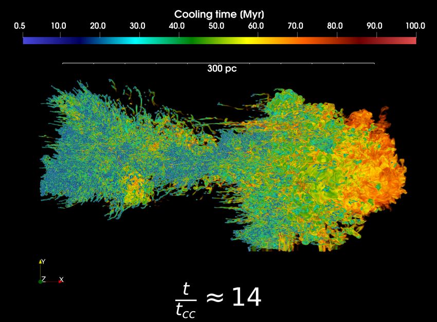
2      Kanjilal, Dutta, Sharma 2020
more recently, Li et al. (2020a) have presented a criterion for cloud      Table 1. Parameters for the cloud-crushing problem
growth that differs qualitatively and quantitatively from Gronke
& Oh (2018). The present work aims to independently study this                 Symbol                              Meaning
important problem.
      While our results are broadly applicable, we choose parame-              Rcl                    Cloud radius (diameter Lcl = 2Rcl )
                                                                               dcell                Cell/grid size in simulation (resolution)
ters relevant for the CGM. Recent observations have revealed the
                                                                               ncl                    Particle number density in the cloud
multiphase structure of the CGM (Tumlinson et al. 2017). The cold
                                                                               nhot                   Particle number density in the wind
phase primarily consists of neutral and low ionization potential ions          Tcl           Temperature of the dense cloud (equals cooling floor)
like H I, Na I, Ca II, and dust; the cool phase harbours ions like C           Thot                       Temperature of the hot wind
                                                                                                                                           √
II, C III, Si II, Si III, N II, and N III; the warm phase is traced by         Tmix          Temperature of the mixed phase, taken to be ThotTcl
high ionization potential ions like C IV, N V, O VI, and Ne VII;               χ                   Wind-cloud contrast (ncl /nhot = Thot /Tcl )
and the hot gas phase by highly ionized species like O VII and                 vwind        Relative speed of the hot wind with respect to the cloud
                                                                                                                                  √
O VIII. The absorption (and less commonly emission) features of                tcc               Classical cloud-crushing time ( χRcl /vwind )
these different species serve as tracers of the multiphase CGM. The            tdrag                        Dragp time (χRcl /vwind )
CGM is polluted by metals due to stellar winds and supernovae,                 M            ≡ vwind /cs ; cs = 1.67P/ρ is hot wind sound speed
which can coalesce at a sufficiently high star formation rate density          tcool,hot                 Cooling time of the hot phase
                                                                               tcool,mix               Cooling time of the mixed phase
(Heckman 2001; Yadav et al. 2017), forming a large-scale galactic
wind. Star formation distributed through the disk can often result
in entrained cold gas moving at high velocity (Cooper et al. 2008;
Vijayan et al. 2018; Schneider et al. 2020), as inferred from spec-        the predictions of Gronke & Oh (2018). According to them, cloud
tral line observations (for a review, see Veilleux et al. 2005; Rupke      growth occurs only if tcool,hot /tlife,pred < 1, where tcool,hot is the
2018). Multiphase gas is seen not only in galactic outflows, but also      cooling time of the hot (not mixed as in Gronke & Oh 2018) phase
in the extended CGM as probed by quasar absorption (Tumlinson              and tlife,pred is a predicted cloud lifetime obtained by fitting their
et al. 2011; Werk et al. 2014). Most likely, this extended multiphase      simulation results to a simple function of the various parameters
gas with a sub-escape velocity is not associated with outflows, but        of the cloud-crushing problem. They estimate the predicted cloud
arises due to condensation induced near wakes of satellite galaxies        lifetime as
and intergalactic filaments on the scale of the halo virial radius (Nel-
son et al. 2020). Cold gas is also seen in cool core clusters within 10s   tlife,pred ≈ 10tcc f ,                                                      (1)
of kpc of the cluster center (e.g., Olivares et al. 2019) and extended
                                                                           where
symmetrically out to the virial radius in z & 3 halos hosting quasars
(e.g., Borisova et al. 2016) and galaxies (e.g., Wisotzki et al. 2018).    f = (0.9 ± 0.1)L10.3 n0.01
                                                                                                 0.3 0.0 0.6
                                                                                                      T6 v100,                                         (2)
      The observations of cold gas moving up to several 100 km
s−1 raise a major question on the existing theoretical models. It          and L1 ≡ Lcl /(1 pc) (Lcl is the initial cloud diameter),
is expected that hydrodynamic instabilities, such as the Kelvin-           n0.01 ≡ nhot /(0.01 cm−3 ), T6 ≡ Thot /(106 K) and v100 ≡
Helmholtz and Rayleigh-Taylor instabilities, should mix the cold           vwind /(100 km s−1 ).
cloud into the diffuse hot phase and ultimately destroy it. The de-             In this paper, we therefore seek to resolve this discrepancy
struction timescale of an adiabatic, initially static cloud of size Rcl    through a set of three-dimensional idealized hydrodynamical sim-
(in pressure equilibrium with its background; Table 1 lists the var-       ulations with radiative cooling, similar to that of Gronke & Oh
ious relevant parameters for the cloud-crushing problem) exposed           (2018, 2020) and Li et al. (2020a), with the simulation parameters
to an impinging hot wind of velocity vwind scales as the cloud-            specifically chosen to address this issue. The paper is organized as
                        √                                                  follows. In section 2 we present the relevant analytical calculations
crushing time tcc ∼ χRcl /vwind (where χ is the density contrast
between the cloud and the wind; Klein et al. 1994). The timescale          to highlight the discrepancy in terms of the initial cloud size. In
of the wind to accelerate the cloud via momentum transfer to speed         Section 3 we describe the simulation details and the range of pa-
∼ vwind is given by the drag time tdrag ∼ χRcl /vwind . Clearly, the       rameters surveyed in our simulations. In Section 4 we present our
                                                      √                    results and discuss their implications. We also present the different
cloud-crushing time tcc is shorter by a factor of χ than the drag
time tdrag , implying that the cloud must be destroyed before it is        diagnostics on the simulated fluid fields to better illustrate the under-
blown away by the wind. This problem – the survival of cool gas            lying physics. In Section 5 we present caveats and future directions.
clouds moving through a hot ambient medium, the cloud-crushing             Finally in Section 6, we summarize our results.
problem, – has received significant attention in recent years, par-        2   Analytic Arguments
ticularly in the context of the CGM (Banda-BarragÃąn et al. 2015;
Schneider & Robertson 2017; Banda-Barragán et al. 2018b; Gronke            According to Gronke & Oh (2018, 2020) cloud growth occurs     √ when-
& Oh 2018, 2020; Sparre et al. 2018; Liang & Remming 2019; Li              ever the cooling time of the mixed gas (evaluated at Tmix ≈ TclThot ;
et al. 2020a; Sparre et al. 2020).                                         see Table 1 for various parameters of the cloud-crushing problem) is
      Recently, Gronke & Oh (2018, 2020) revisited the problem             shorter than the cloud-crushing time; i.e., tcool,mix /tcc < 1. In terms
of entrainment of hot wind by a cold cloud and derived a crite-            of the initial cloud radius, this criterion corresponds to a cloud size
rion for cloud growth due to radiative cooling. They concluded that        larger than
whenever the ratio of the cooling time of the mixed gas and the                                 5                             3
                                                                                               2                       2
cloud-crushing time (tcool,mix /tcc ) < 1, the mixed warm gas pro-                           Tcl,4 M χ               Tcl,4 M       χ
                                                                           RGO ≈ 2 pc                   = 2 pc                        ,                (3)
duced in the boundary layer cools and produces new comoving cold                      P3 Λmix,−21.4 100        ncl,0.1 Λmix,−21.4 100
gas, and thus, the cloud grows and acquires momentum. More re-
cently, however, Li et al. (2020a) derived a criterion for cold mass       where Tcl,4 ≡ (Tcl /104 K), P3 ≡ nT/(103 cm−3 K), Λmix,−21.4 ≡
growth due to radiative cooling and it is somewhat different from          Λ[Tmix ]/(10−21.4 erg cm3 s−1 ), and ncl,0.1 ≡ (ncl /0.1 cm−3 ). Recall

                                                                                                                             MNRAS 000, 1–14 (2020)
Multiphase gas in the cloud-crushing problem with cooling 3
Gronke-Oh Radius (pc) [log] Li Radius (pc) [log] log10(RGO/RLi)
-0.2 0.0 0.2 0.4 0.6 0.5 1.0 1.5 2.0 2.5 -2.0 -1.5 -1.0 -0.5
1.5 0.6
0.15
00
1.500
2.000
0.500
2.500
-2.000
-1.200
0
-0.400
0.30
1.000
0.0
1.0 0.4
0
-0.800
00
50
-0.
1
00
50
0.5
-1.6
100 200 300 100 200 300 100 200 300
χ χ χ
Figure 1. The Gronke-Oh radius (log; Eq. 3; left panel), the Li radius (log; Eq. 5; middle panel), and their ratio (right panel) as a function of the density contrast
χ and the Mach number M. The variation of the two radii as a function of χ and M is different qualitatively and qauntitatively. We vary these two parameters
(χ, M) in our cloud-crushing simulations with cooling to test the two criteria for the growth of cold/dense gas. For most of the relevant parameter regime, the
Li radius exceeds the Gronke-Oh radius by more than a factor of 10, with the discrepancy increasing with χ.
that the cooling time is origin. Notice that the cooling times tcool,mix and tcool,hot , in terms
3 k BT of the cloud-crushing parameters (ncl , Tcl , M, χ, Rcl ), depend on
tcool ≡ , (4) ncl , Tcl and χ, tcc on Rcl , M and Tcl , and tlife,pred on all of them
2 nΛ [T]
except χ. The three colored solid lines in Figure 2 show the Gronke-
where Λ[T] is the cooling function such that the energy loss due to Oh criterion in terms of tcool,hot and tlife,pred for three different Mach
radiative cooling per unit volume for a given number density and numbers, and for ncl = 0.1 cm−3 and Tcl = 104 K. For each of these
temperature is given by n2 Λ[T]. curves, we fix M, ncl and Tcl and vary χ. For each χ there is a unique
In contrast, Li et al. (2020a) claim that cloud growth due to ra- threshold radius corresponding to the Gronke-Oh criterion (Eq. 3),
diative cooling occurs when tcool,hot /tlife,pred = tcool,hot /(10tcc f ) < and hence a unique tlife,pred . Note that at small values of tcool,hot ,
1 (see section 3.4 and Eq. 19 in Li et al. 2020a). The radius accord- different values of χ can give the same tcool,hot k but different RGO
ing to this criterion for cold gas growth, expressed in terms of the and tlife,pred . Again notice that the Gronke-Oh and Li criteria are
same parameters as Eq. 3, should exceed (using Eqs. 1, 2) qualitatively and quantitatively very different, with the difference
12
13
4 increasing with an increasing χ (consistent with the right panel of
Tcl,4 M 13 χ 20
RLi ≈ 15.4 pc
13
, (5) Figure 1).
10
13 100
ncl,0.1 Λhot,−21.4 3 Numerical Simulations
Now that we have highlighted the large discrepancy between the
where Λhot,−21.4 ≡ Λ(Thot )/(10−21.4 erg cm3 s−1 ). Note that the
analytic Gronke-Oh and Li criteria for cold cloud growth in the
cooling function in Eqs. 3 & 5 are evaluated at Tmix and Thot , respec-
cloud-crushing problem with cooling, we turn to numerical simu-
tively. For typical values of the parameters, Tcl = 104 K, M = 1.0,
lations to check whether they agree with any of these criteria.
χ = 100, and ncl = 0.1 cm−3 , the corresponding Gronke-Oh and
Li radii are approximately 1.1 pc and 26.5 pc, respectively. Thus, We set up three-dimensional hydrodynamical simulations in
there exists a major discrepancy between the two criteria. Figure 1 a uniform (∆x = ∆y = ∆z = dcell ), Cartesian grid corresponding
shows the Gronke-Oh and Li radii, and their ratio as a function of to the classical cloud-crushing scenario along with optically thin
the density contrast ( χ) and the Mach number (M) for a fixed cloud radiative cooling of collisionally ionized gas similar to Gronke &
temperature Tcl = 104 K and density ncl = 0.1 cm−3 . By comparing Oh (2018, 2020). Since the physical set up is well-known, we do
Eqs. 3 & 5, note that the ratio is independent of the cloud density not repeat all the details here and just present the key highlights. We
but depends on the other parameters. implement our numerical experiments in PLUTO 4.3, a conservative
Figure 2 shows a comparison of the Gronke-Oh and Li criteria Godunov hydrodynamics code (Mignone et al. 2007). We place a
for the growth of cold gas in the cloud-crushing problem, expressed dense, spherical cloud of cold gas of radius Rcl at a temperature of
in terms of the key parameters of Li et al. (2020a), tcool,hot (the Tcl = 104 K and number density ncl = 0.1 cm−3 in our simulation
cooling time of the hot wind) and tlife,pred (the predicted lifetime in domain and impose a steady hot wind outside it. All the boundaries
the cloud-crushing problem; see Eqs. 1 & 2).¶ In this space, the Li
criterion is simply given by a line of slope unity passing through the
simulation parameters (χ, M, ncl , Tcl ) and we did not want to misquote
their results.
¶ We use tlife,pred − tcool,hot coordinates suggested by Li et al. (2020a) k This happens below χ ≈ 2, where the cooling function is locally steeper
for a comparison because we were not readily able to get their individual than T 2 .
MNRAS 000, 1–14 (2020)
4                      Kanjilal, Dutta, Sharma 2020
                          5
                                 Gronke-Oh Criterion for = 0.5                                   Table 2. Various code parameters†
                                 Gronke-Oh Criterion for = 1.0
                                 Gronke-Oh Criterion for = 1.5
                          4      Li Destroyed Clouds
                                 Li Growing Clouds                                                       Geometry                                           Cartesian
                                 Growing Clouds in Our Simulations for = 0.5                             Solver                                                HLLC
                          3      Growing Clouds in Our Simulations for = 1.0
                                 Growing Clouds in Our Simulations for = 1.5                             Cooling                 Tabulated function (solar metallicity)
                                 Destroyed Clouds in Our Simulations for = 1.0                           Flux form                                Dimensionally-split
log10 tlife, pred [Myr]

                                 Li Criterion
                          2                                                                              External forces                                       Absent
                                                                                                         Thermal Conduction                                    Absent
                          1                                                                              Self-gravity                                          Absent
             )

                                                                                                         Reconstruction                                   Linear TVD
                                                                                                         Time stepping                                            RK2
                          0
                                                                                                         Viscosity                        Non-explicit code viscosity
             (

                                                                                                         Equation of state                         Ideal gas, γ = 5/3
                          1                                                      = 300
                                                                                                         CFL limiting value                                         0.2
                                                                    = 100
                          2                                                                      †   see the PLUTO code manual (v4.3) for details.

                          3
                                                                                                 physical and numerical options implemented in our simulations.
                                                                                                 Most of our simulations are run for a timescale shorter than the
                          42          1           0           1             2    3       4   5   cooling time of the hot wind because we wish to study the cooling
                                                      log10(tcool, hot) [Myr]                    of the mixed gas produced in the boundary layer. For the CGM
                                                                                                 one also has to worry about the thermodynamics of the diffuse hot
       Figure 2. The results of our cloud-crushing simulations (colored open sym-
                                                                                                 phase, which is beyond the scope of the present work.
       bols) superimposed on the points taken from the bottom panel of Figure 3
       in Li et al. (2020a) (grey filled symbols). Circles denote the runs where the
                                                                                                       We initialize the setup in pressure equilibrium. The Mach num-
       dense gas is ultimately destroyed and triangles where it grows. The dashed                ber of the background wind is chosen from M = {0.5, 1.0, 1.5} and
       line shows the Li criterion for the growth of clouds in the cloud-crushing                the density contrast from χ = {100, 300} to cover a considerably
       problem and the three colored solid lines show the Gronke-Oh criterion for                wide range in the parameter space relevant to the CGM. For a par-
       different Mach numbers. Our simulation symbols are colored according to                   ticular combination of M and χ (and our fixed ncl and Tcl ), we
       the Mach number of these lines. We find cloud growth in the region be-                    obtain the corresponding Gronke-Oh and Li radii, RGO and RLi ,
       tween the Li and the Gronke-Oh thresholds, and cloud destruction occurs                   from Eq. 3 and Eq. 5 respectively. Since numerical experiments
       below the Gronke-Oh threshold. Notice the red open circle lying above the                 with cloud sizes between the Gronke-Oh and Li radii are essential
       Gronke-Oh radius for M = 1 (solid red line), indicating a cloud larger than               to resolve the discrepancy between the two criteria, we parameterize
       RGO showing dense mass destruction; this is perhaps a result of insufficient
                                                                                                 the cloud size as
       resolution (see Appendix B). Our simulations shown in this plot correspond
       to a density contrast of either χ = 100 or χ = 300. All our simulations and                         β   1−β
                                                                                                 Rcl = RLi RGO ,                                                          (6)
       the three solid lines use ncl = 0.1 cm−3 and Tcl = 104 K (these line move
       down/up with an increasing/decreasing ncl ).                                              where we choose the "interpolation parameter" βs between 0.3 and
                                                                                                 1 for the runs with RGO ≤ Rcl ≤ RLi . The cloud size between the
                                                                                                 Gronke-Oh and Li radii correspond to 0 < β < 1, with a smaller β
       are outflowing except the one in the upstream direction where we                          corresponding a smaller size closer to the Gronke-Oh radius (which
       impose a constant inflow of the hot gas at a fixed density, temperature                   is always smaller than the Li radius for parameters of interest). We
       and velocity (as measured in the lab frame).                                              also carry out a few runs with clouds smaller than the Gronke-
             We use a cloud-tracking scheme which continuously changes                           Oh radius and verify that the clouds smaller than this are indeed
       the frame of reference so that we can follow the cloud gas (tagged                        destroyed. Table 3 lists the various parameters – χ, M, Rcl and β –
       by a passive scalar) and prevent it from quickly moving out of the                        for our different simulations.
       box (Shin et al. 2008; Dutta & Sharma 2019). Nevertheless, we
       still we use fairly long boxes to prevent the cloud-wind interaction                      4     Results and Discussion
       region from moving out of the computational domain. The typical                           In this section, we discuss the results of our numerical simulations
       box-size for our simulations is 400 Rcl along the wind direction                          designed to distinguish between the Gronke-Oh and Li criteria for
       and 30 Rcl in the orthogonal directions. This box is large enough                         the growth of cold gas in the cloud-crushing problem with cooling.
       such that the passive scalar (marking the initial cloud) does not leak                          Figure 3 shows the mid-plane density (left panels), passive
       out of the boundaries (this is ensured by monitoring the volume                           scalar concentration (middle panels), and pressure (right panels)
       integral of the passive scalar). We primarily focus on simulations                        slice plots for the fiducial run with χ = 100, M = 1 and Rcl = 14
       with a resolution of Rcl /d cell = 8, but we also perform simulations                     pc, which is predicted to grow according to the Gronke-Oh criterion
       up to Rcl /d cell = 64 (this high resolution run has a smaller box-size                   but not according to the Li criterion. These snapshots are made for
       30Rcl × 15Rcl × 15Rcl ). Appendices A & B study the impact of the                         the highest resolution run with Rcl /dcell = 64 but a smaller box-
       box-size and resolution, respectively.                                                    size 30Rcl × 15Rcl × 15Rcl rather than for the standard runs with
             We use a tabulated cooling function generated by CLOUDY                             larger boxes to better visualize the small-scale features. The price
       (Ferland et al. 2017) for a solar metallicity plasma (Asplund et al.                      we pay is that a part of the turbulent mixing layer moves out of the
       2009) assuming collisional ionization equilibrium. This cooling                           computational domain.
       table is available with the publicly available version of the PLUTO                             With time in Figure 3, we see the formation of a turbulent
       code. We set the cooling function to zero below Tcl to crudely mimic                      wake with intermediate densities and intermediate passive scalar
       heating due to the UV background. In Table 2 we list the various                          concentrations. While pressure is uniform in the initial state, a bow

                                                                                                                                                  MNRAS 000, 1–14 (2020)
Multiphase gas in the cloud-crushing problem with cooling 5
Table 3. Physical & numerical parameters of our different runs
χ M Rcl β Cooling tcc tcool,mix Rcl /dcell box-size in Boundary Cloud
(pc) (Eq. 6) (Myr) (Myr) Rcl (L,T,T) Condition (T) Growth
100† 1.0 14.0 0.8 yes 0.96 0.09 8,16,32 (400,30,30) outflow yes
100† 1.0 14.0 0.8 yes 0.96 0.09 64 (30,15,15) outflow yes
100 1.0 5.47 0.5 yes 0.37 0.09 8 (400,30,30) outflow yes
100 1.0 2.90 0.3 yes 0.19 0.09 8 (400,30,30) outflow no
100 1.0 1.0 -‡ yes 0.07 0.09 8 (400,30,30) outflow no
100 1.0 0.5 - yes 0.03 0.09 8 (400,30,30) outflow no
100 1.0 14.0 0.8 no 0.96 - 8 (400,30,30) outflow no
100 1.0 5.47 0.5 no 0.37 - 8 (400,30,30) outflow no
100 1.5 17.0 0.8 yes 0.78 0.09 8 (400,30,30) outflow yes
100 1.5 7.16 0.5 yes 0.33 0.09 8 (400,30,30) outflow yes
100 0.5 10.36 0.8 yes 1.42 0.09 8 (400,30,30) outflow yes
100 0.5 3.49 0.5 yes 0.48 0.09 8 (400,30,30) outflow yes
300 1.0 169.02 0.8 yes 11.58 0.25 8 (400,30,30) outflow yes
300 1.0 37.64 0.5 yes 2.58 0.25 8 (400,30,30) outflow yes
300 1.0 2.8 - yes 0.19 0.25 8 (400,30,30) outflow no
300 1.0 1.5 - yes 0.10 0.25 8 (400,30,30) outflow no
300 1.5 202.45 0.8 yes 9.24 0.25 8 (400,30,30) outflow yes
300 1.5 49.01 0.5 yes 2.24 0.25 8 (400,30,30) outflow yes
300 0.5 124.06 0.8 yes 16.99 0.25 8 (400,30,30) outflow yes
300 0.5 23.92 0.5 yes 3.28 0.25 8 (400,30,30) outflow yes
50 1.0 6.79 - yes 0.46 0.07 8 (400,30,30) outflow no
100 1.0 26.5 1.0 yes 1.82 0.09 8 (20,10,10) periodic yes
100 1.0 14.0 0.8 yes 0.96 0.09 8 (400,30,30) periodic yes
100 1.0 14.0 0.8 yes 0.96 0.09 8 (200,10,10) periodic yes
100 1.0 14.0 0.8 yes 0.96 0.09 8 (100,10,10) periodic yes
100 1.0 14.0 0.8 yes 0.96 0.09 8 (20,10,10) periodic yes
100 1.0 10.28 0.7 yes 0.70 0.09 8 (20,10,10) periodic yes
100 1.0 7.5 0.6 yes 0.51 0.09 8 (20,10,10) periodic yes
100 1.0 6.4 0.55 yes 0.44 0.09 8 (20,10,10) periodic no
100 1.0 5.47 0.5 yes 0.37 0.09 8 (100,10,10) periodic yes
100 1.0 5.47 0.5 yes 0.37 0.09 8 (20,10,10) outflow no
100 1.0 5.47 0.5 yes 0.37 0.09 8 (20,10,10) periodic no
† The fiducial runs (different versions differ by resolution and box-size). ‡ For Rcl < RGO (Eq. 3) or Rcl > RLi (Eq. 5), we do not specify β.
The longitudinal boundary conditions are outflow in the downstream direction and wind parameters are imposed in the upstream direction.
shock is formed ahead of the cloud that becomes weaker with time probability distribution functions (PDFs) of the different fluid fields
because of momentum transfer between the wind and the cloud. and elucidate the physics of the turbulent multiphase wake.
The bow shock quickly moves out of the computational domain. At
4.1 Cloud survival & growth
late times, the turbulent wake becomes long and filamentary, with
the intermediate density clouds cooling and falling on to the tail. The left panel of Figure 4 shows the dense mass (all the mass in grid
The cooler portions of the wake collapse on to the filamentary tail, cells with density ρ > ρcl /3) evolution for all the simulations with
which has a smaller pressure, in form of a quasi-steady, pressure- Rcl /d cell = 8, the box-size (400, 30, 30)Rcl , and outflow boundary
driven cooling flow (Dutta et al. in prep.). Such a collapse of the condition in the transverse direction. In absence of cooling, the
wake is not observed in the simulations with weak cooling in which cold/dense cloud is mixed into the hot/dilute phase in a few cloud-
the cold gas is eventually completely destroyed. Notice the flaring crushing times. The cloud material becomes comoving with the
of the turbulent tail at the end, very clearly seen in the passive scalar wind on a much longer (by ∼ χ1/2 ) drag timescale.
snapshots. Similar features are observed in our low resolution simu- In simulations with cooling, eventually the clouds enter a phase
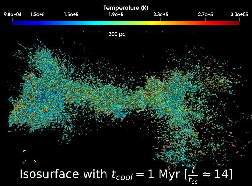
lations but obviously not in this great detail. Appendix C shows that of mass growth if the cloud size is larger than the Gronke-Oh radius
the surfaces with the shortest cooling times are highly corrugated, (Eq. 3). The simulations with a smaller cloud radius or without
with a fractal-like structure. cooling eventually show the destruction of cold gas. Since our 0 <
β < 1 runs (corresponding to a cloud radius smaller than the Li
Now that we have looked at the evolution of the morphology of radius but larger than the Gronke-Oh radius) show cloud growth,
the wake in the cloud-crushing problem with cooling, we study the they are consistent with Gronke & Oh (2018, 2020) and disagree
effects of different parameters on cloud survival and compare our with the Li criterion (Eq. 5).
result with the Gronke-Oh and Li survival criteria. In this context, If cooling is efficient in the mixed gas formed by shear between
we look at some of the standard volume-integrated diagnostics that the cloud and the wind, the mixed warm gas at the peak of the cooling
quantify the mass growth of the dense/cold gas and momentum curve can cool and accrete on to the cold tail and the dense mass
transfer (entrainment) between different phases in our simulations. can grow. Initially, due the turbulent instabilities and mixing, the
We analyze the statistical properties of the multiphase wake using cloud loses mass, which is clearly observed in the plot till t ≈ 3tcc
MNRAS 000, 1–14 (2020)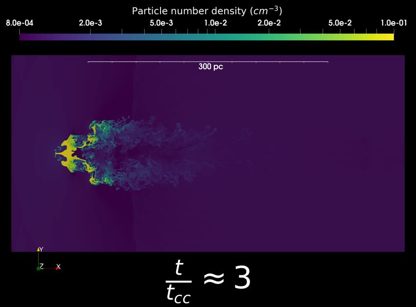
6      Kanjilal, Dutta, Sharma 2020

Figure 3. The density (left panels), passive scalar (middle panels), and pressure (right panels) slices in the x − y plane through the center at different times for
our fiducial high resolution simulation (Rcl = 14 pc, Rcl /dcell = 64; see Table 3). The initial pressure is uniform but a bow shock forms as the wind interacts
with the stationary cold cloud. The mixing and cooling in the boundary layer leads to the growth of cold gas and entrainment of the cold gas by the wind at
late times. Notice the dense clumps falling on to the filamentary tail at late times and the flaring of the tail at its end. The dense tail has a passive scalar value
. 0.3 at t = 14tcc , indicating that most of this gas originates in the hot wind.

(later for smaller clouds). But for clouds larger than the Gronke-Oh                        The right panel of Figure 4 shows the evolution of the relative
radius, the cold gas mass increases at later times. The cold gas mass                 velocity between the wind and the cloud gas as a function of time
at t ≈ 18tcc for some of the larger clouds is significantly larger than               for the simulations shown in the left panel. Recall that the initial
the initial cloud mass. In contrast to the cloud-crushing simulations                 cloud is traced by a passive scalar C, which is set to unity for the
without cooling or with inefficient cooling, for Rcl > RGO the mixed                  cloud and to zero for the wind. Therefore the cloud material velocity
warm gas in the boundary layer cools efficiently, creating thermal                    at any time is given by
pressure gradients that enable further inflow of hot gas into the
                                                                                                                       ρCvdV
                                                                                                                   ∫
mixing layer. This continuously fed cooling layer entrains the hot                                                  ∫V        ,
wind and leads to the growth of the dense mass.                                                                      V
                                                                                                                        ρCdV
                                                                                      and the wind velocity by
4.2   Momentum exchange & cold mass entrainment
                                                                                                                            ρ(1 − C)vdV
                                                                                                                    ∫
In the cloud-crushing problem in absence of cooling, the timescale                                                   ∫V                   ,
for momentum exchange between the cloud and the wind material                                                           V
                                                                                                                            ρ(1 − C)dV
is tdrag ∼ χRcl /vwind , which is longer than the cloud-crushing time                 where v is the fluid velocity, ρ is the mass density, and V denotes
by a factor ∼ χ1/2 . This means that the cloud mixes in the hot                       the computational volume. We plot the difference between the wind
wind before it can be pushed substantially by it. The cloud-crushing                  and cloud velocities normalized by the initial wind speed versus
time scales as the Kelvin-Helmholtz instability growth timescale                      time normalized by the classical drag time tdrag (see Table 1).
and the drag timescale corresponds to the time over which the cloud                        Similar to Gronke & Oh (2018, 2020), we find that entrain-
encounters its own mass in the hot wind. The drag timescale can                       ment indeed happens on a characteristic timescale ∼ tdrag , the same
also be motivated from the Rayleigh drag formula applicable for                       timescale as in the absence of cooling. Thus cooling does not really
a turbulent wake; namely the drag force acting on the cold cloud                      affect the momentum exchange between the cold and hot phases
         2 v2
∼ ρhot Rcl       .                                                                    but fundamentally changes the mass exchange. Even for a cloud
            wind

                                                                                                                                              MNRAS 000, 1–14 (2020)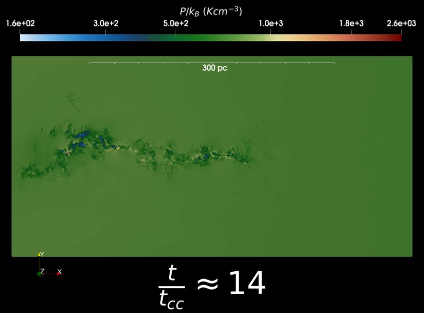
Multiphase gas in the cloud-crushing problem with cooling 7
( , , Rcl[pc]) ( , , Rcl[pc])
(100,1.0,14.0)
(100,1.0,5.47) 1.0 (100,1.0,14.0)
(100,1.0,5.47)
(100,1.0,2.9) (100,1.0,2.9)
Dense Mass, M > 3cl /Mcl, 0
(100,1.0,1.0) (100,1.0,1.0)
(100,1.0,0.5) (100,1.0,0.5)
101 (100,1.0,14.0), No Cooling
(100,1.0,5.47), No Cooling 0.8 (100,1.0,14.0), No Cooling
)
(100,1.0,5.47), No Cooling
(100,1.5,17.0) (100,1.5,17.0)
(100,1.5,7.16) (100,1.5,7.16)
(100,0.5,10.36) (100,0.5,10.36)
(100,0.5,3.49)
0.6 (100,0.5,3.49)
(
(300,1.0,169.02) (300,1.0,169.02)
vwind
v
(300,1.0,37.64) (300,1.0,37.64)
100 (300,1.0,2.8)
(300,1.0,1.5)
(300,1.0,2.8)
(300,1.0,1.5)
(300,1.5,202.45) (300,1.5,202.45)
(300,1.5,49.01) 0.4 (300,1.5,49.01)
(300,0.5,124.06) (300,0.5,124.06)
(300,0.5,23.92) (300,0.5,23.92)
10 1 0.2
0 5 10 15 20 25 30 0.00 0.25 0.50 0.75 1.00 1.25 1.50
t t
tcc tdrag
Figure 4. Left: The mass evolution of the dense gas (ρ > ρcl /3) for our runs with various density contrasts (χ), initial cloud radii (Rcl ), and the wind Mach
number (M). The mass is normalized to the initial cloud mass. The runs without cooling show cloud destruction after a few cloud-crushing times (Klein et al.
1994). Even with radiative cooling, clouds smaller than the Gronke-Oh radius do no show cold mass growth. Larger clouds show an initial dip in the dense
mass but it grows later as gas from the hot wind is mixed and cooled into the dense tail (see the bottom panels of Figure 3). The green solid line corresponds
to the red circle in Figure 2 above the red solid line for a cloud larger than the Gronke-Oh radius. Dense mass show slight increase before dissolving into the
hot wind due to insufficient resolution (see the left panel of Figure B1). Right: The speed difference between the wind and the cloud material normalized
by the initial wind speed. The black crosses indicate the times when the cold mass gets completely destroyed due to mixing with the hot wind. The decrease
in the speed difference indicates momentum transfer due to turbulent mixing between the two phases with an initial velocity difference. Somewhat shallower
evolution in some of the runs with cooling may be because of insufficient resolution (see the right panel of Figure B1).
larger than the Gronke-Oh radius, the mixing between the phases 4.4 Cloud Dynamics: A detailed look
occurs on the Kelvin-Helmholtz timescale. However, in contrast to The turbulent mixing layer, with gas at intermediate tempera-
cloud-crushing without cooling where mass transfer happens from ture/density/velocity, is an essential element of the dynamics of
the cold to the hot phase, the mass transfer is in the opposite di- cloud-crushing both with and without cooling. In absence of cool-
rection for cloud-crushing with a cloud larger than the Gronke-Oh ing, the turbulent boundary layer grows with time and the cold phase
radius. This qualitative change happens because the mixed gas has a is mixed in the hot wind after a few cloud-crushing times. However,
cooling time shorter than the turbulent mixing time. In the absence the cloud material, which is mixed in the hot wind, takes a longer
of cooling, mixing leads to the turbulent evaporation of the cold time (tdrag ∼ χ1/2 tcc ) to become comoving. Thus there is mass
cloud as it continuously encounters the hot wind. The physics of transport from the cold to hot phase on ∼ tcc timescale and momen-
momentum exchange between the hot and the cold phases remains tum transfer from the hot to cold phase on ∼ tdrag . With cooling, for
unchanged and the two phases again become comoving after the a sufficiently large cloud, the net mass transfer reverses and is from
cold cloud encounters roughly its own mass in the hot wind. hot to the cold phase because the mixed layer can cool and accrete
on to the cold filamentary tail.
Begelman & Fabian (1990) consider a mixing layer which
entrains mass from the hot and cold phases such that the mean
4.3 Dependence on density contrast & Mach number
temperature of the mixed phase is
MÛ T + MÛ clTcl p
In absence of radiative cooling, all clouds are expected to mix into Tmix ∼ hot hot ∼ ThotTcl, (7)
the diffuse hot phase over a few tcc . Radiative cooling allows the MÛ hot + MÛ cl
possibility of the growth of cold mass, provided the cloud radius is where MÛ hot and MÛ cl are the mass entrainment rates into the mixed
large enough. The Gronke-Oh radius (Eq. 3) is larger for a larger layer from the hot and cold layers, respectively. This estimate as-
density contrast and a higher Mach number. This implies that the sumes that MÛ cl / MÛ hot ∼ vin,hot /vin,cl ∼ χ1/2 (vin,cl [vin,hot ] is the
clouds with smaller χ and M grow faster, as is borne out by the left inflow velocity from the cold [hot] phase into the mixing layer).
panel of Figure 4. These scalings also imply that the mixed layer’s longitudinal veloc-
The right panel of Figure 4 shows that the cloud material be- ity is close to the longitudinal velocity of the cold gas.
comes comoving in all cases after about a drag time, irrespective of Gronke & Oh (2018) used the above scalings for a turbulent
whether the cold mass grows or the cold gas is destroyed. There are boundary layer to understand their numerical simulations of cloud-
no significant trends with the density contrast and the Mach num- crushing problem with cooling. √ The cold cloud can grow if the
ber. The simulations with faster cooling show a longer acceleration mixed gas, assumed to be at ∼ TclThot cools faster than the cloud-
timescale for the cold cloud but this is likely a numerical artifact crushing time, the timescale over which the cold cloud is mixed into
due to insufficient resolution (see B). the hot wind in absence of cooling. While this scaling is reasonable
MNRAS 000, 1–14 (2020)
8 Kanjilal, Dutta, Sharma 2020
102
for a cooling function that peaks at the intermediate temperatures t=0 t=0
101 t tcc 101 t tcc
(which is true for the typical CGM/galactic outflow parameters), it t 3 tcc t 3 tcc
must be refined for a qualitatively different cooling function. 100 t 6 tcc t 6 tcc
t 12 tcc 10 1 t 12 tcc
10
M0 d(log10T)
1 t 18 tcc
t 18 tcc
V0 d(log10T)
4.4.1 1-D Probability distribution functions
1 dM
1 dV
10 2
Probability distribution function (PDFs) are commonly used to de- 10 3
10 3
scribe the statistical properties of turbulent flows (e.g., Pope 2000).
10 4
Figure 5 shows some useful PDFs at different times for the fiducial 10 5
cloud-crushing simulation with Rcl /dcell = 8 (see Table 3). The top 10 5
left panel shows the mass-weighted temperature PDF (mass filling 10 63.5 4.0 4.5 5.0 5.5 6.0 10 73.5 4.0 4.5 5.0 5.5 6.0
fraction) and the top right panel shows the volume-weighted PDF log10(T[K]) log10(T[K])
102
(volume filling fraction). The bottom left panel is the volume PDF t=0 t=0
t tcc 1036 t tcc
of pressure and the bottom right panel shows the differential cooling 100 t 3 tcc t 3 tcc
t 6 tcc
dlog10T (ergs )
rate at different temperatures in the simulation domain. t 6 tcc
1
t 12 tcc t 12 tcc
V0 d(log10P)
The temperature PDFs appear as two sharp peaks at t = 0. The 10 2 t 18 tcc 1034 t 18 tcc
1 dV
amplitude of the low-temperature peak in the temperature PDFs
(marking the cold gas) falls and broadens during the early times 10 4
1032
dEcool
because of turbulent mixing. This cold peak undergoes a significant
10 6
rise at later times due to the cooling of the mixed gas and the
1030
subsequent cold mass growth. The volume and mass of the gas 10 8
2.0 2.5 3.0
at intermediate temperatures also rise with time due to turbulent
mixing and cooling.
log10 kPB [Kcm 3]
( )
3.5 4.0 4.5 5.0
log10(T[K])
5.5 6.0
Notice that the hot peak moves to the lower temperatures (ac- Figure 5. Some useful PDFs at different times for our fiducial simulation
companied by a movement to low pressure as seen in the pressure at the resolution of Rcl /dcell = 8 (see Table 3). The counting uncertainty
PDF) as the runtime approaches the cooling time of the diffuse hot in each bin of the PDFs√is assumed to follow a Poisson statistic and hence
wind. After this time we expect the whole computational box to a shaded spread ∝ 1/ bin count − 1 is marked for every bin. Top left:
cool to the cooling floor. While the cooling time of the background The mass-weighted PDF (mass-filling fraction) of temperature shows the
hot gas in the central CGM can be much shorter than the Hubble cold and the hot phases. Because of the large box-sizes in our simulations,
time and it is important to study its thermodynamics (e.g., Sharma the mass fraction of the hot phase is much higher than the cold phase.
2018), in this paper we only focus on the cooling of the turbulent With time, turbulent mixing and cooling create intermediate temperature
phases. In absence of cooling, the cold peak mixes into the hot one in a
boundary layers.
few tcc . Background cooling results in the slight shift of the hot phase peak
The pressure PDF, unlike temperature, has a single peak, indi-
to lower temperature values at late times. Top right: Time evolution of
cating that the conditions remain nearly isobaric. Although localized the volume-weighted PDF (volume-filling fraction) of temperature. Bottom
regions at intermediate temperatures can cool faster than the sound- left: The volume-weighted PDF of pressure shows only one peak and no
crossing time, for most of the volume and time cooling is subsonic. additional peaks develop with time. This shows that mixing and cooling
The low-pressure tail at late times corresponds to the filamentary in the boundary layer occur in approximately isobaric conditions. The low
cold tail as seen in the lower panels of Figure 3. pressure tail corresponds to the cold gas formed in the turbulent cooling
The bottom-right panel of Figure 5 shows the radiative cooling wake. The high pressure tail at early times is produced mainly by the gas
losses (assuming optically thin conditions) as a function of the gas crossing the bow shock and at late times by the transient shocks forming
temperature.∫We obtain d EÛcool /d log10 T by calculating the cooling around cooling blobs (see the right panels of Figure 3). Once again note
that background cooling drives the pressure peak to smaller values. Bottom
losses EÛ = V n2 Λ(T)dV as a function of temperature distributed
right: The differential cooling rate at different temperatures. The hot gas,
across uniform bins in log10 T. The radiative cooling PDF also has
which fills most of the simulation volume, naturally causes a large peak
two peaks at all times, corresponding to the hot and the cold phases. at the high temperature. This peak slightly shifts to the left with time due
Although the mass and volume in the intermediate temperatures is to the cooling of the background hot gas. Cooling losses at intermediate
low, the cooling rate at these temperatures is significant because the temperatures are significant, and the features in the differential cooling
cooling function peaks at these temperatures (∼ 105 K). losses reflect the interplay between turbulent mixing and cooling moving the
gas across temperatures. The differential emission measure is qualitatively
4.4.2 Comparison with a simple cooling flow
different from a simple steady cooling flow (see section 4.4.2 for details).
Figure 6 shows the analytic isobaric and isochoric cooling times as
a function of temperature,
2 2
5 k BT as a function of temperature at different times (dashed lines). We
tcool,IB = (8)
2p Λ(T) shade the 1 − σ spread of the cooling time for t ≈ 18tcc .
and We find that the cooling time from the simulation matches very
well with the isobaric cooling time using a pressure lower than the
3 k BT
tcool,IC = . (9) initial pressure. This again reflects the smaller pressure and isobaric
2 nΛ(T) conditions in the cooling turbulent boundary layer. The various
For the figure, the pressure and density in the above equations are bumps and wiggles in the cooling time reflect the similar features
chosen to match the conditions at 18tcc ; the density for the isochoric in the cooling curve. Note that the cooling time versus temperature
cooling time (solid blue√line) is adjusted to cross the isobaric cooling is not as smooth at early times but the variations are smoothed out
time (solid red line) at TclThot = 105 K. The isobaric cooling time with time.
at the large-scale ambient pressure is shown with a red solid line. We While Figure 6 clearly indicates isobaric conditions in the
also plot the median cooling time across the computational domain cooling boundary layer, the energy radiated by gas at different tem-
MNRAS 000, 1–14 (2020)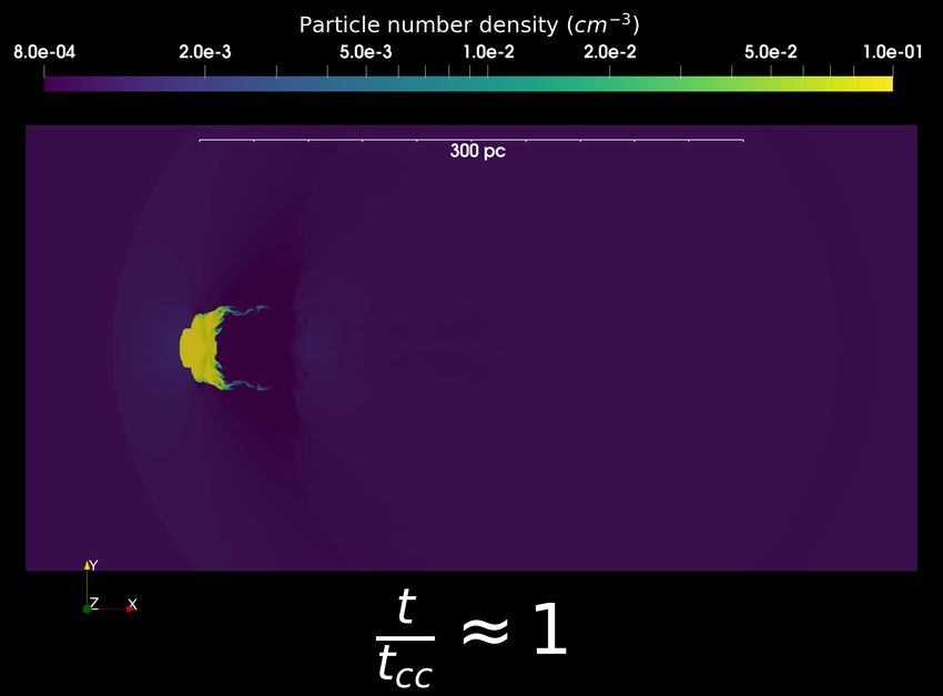
Multiphase gas in the cloud-crushing problem with cooling                           9

                               t tcc                                                   indicate the locations of peaks in the initial PDFs. At t = 0 the
                     104       t 6tcc                                                  cold cloud and the hot wind have the same pressure, temperatures
                               t 18tcc                                                 differing by χ = 100, and speeds differing by vwind ≈150 km s−1 .
                               Isobaric Cooling, (P/kB) = 241.33 Kcm 3                       In absence of radiative cooling (not shown) the low temperature
                     103       Isobaric Cooling, (P/kB) = 680.16 Kcm 3                 peak completely merges into the hot peak by a few tcc (see the dotted
                               Isochoric Cooling, n = 1.45 × 10 3cm 3                  lines in the left panel of Figure 4). However, with cooling and for
Cooling Time (Myr)

                                                                                       Rcl > RGO , the cold gas is replenished by the cooling of the mixed
                     102                                                               phase and hence the peak at Tcl is seen at all times. The spread in
                                                                                       pressure values of all the fluid elements as illustrated in the joint
                                                                                       PDFs the joint PDFs (left panels) is larger at early time because of
                                                                                       a strong bow shock, rarefaction, and fast cooling of the mixed gas
                     101                                                               (see the right panels of Figure 3). At late times, the pressure is more
                                                                                       uniform, with a slight dip close to the cloud temperature, indicating
                                                                                       a pressure-driven turbulent cooling flow on to the dense tail.
                     100                                                                     The high velocity peak in the relative speed-temperature PDF
                                                                                       slowly moves to lower velocities and fully crosses 100 km s−1 by
                                                                                       12 tcc , which is of order the drag time. Thus, in agreement with the
                10     1
                                                                                       right panel of Figure 4, the cold gas starts to become comoving with
                                                                                       the hot wind after roughly a drag time. Once the hot and cold phases
                                                                                       do not have a relative speed, the turbulent cooling boundary layer
                       3.5     4.0       4.5      5.0       5.5          6.0   6.5
                                             log10T(K)                                 is expected to decay as shear driven turbulence gradually weakens.
                                                                                       4.5   Resolving the Gronke-Oh & Li discrepancy
      Figure 6. The median cooling times at different temperatures for the fiducial
      simulation (Rcl /dcell = 8; see Table 3) at different times are represented by   The key aim of this paper is to reconcile the large discrepancy
      the dashed lines. For t ≈ 18tcc we also show the 1 − σ spread around the         in the Gronke-Oh and Li criteria, expressed most transparently in
      median value. The solid lines show the analytic isobaric (Eq. 8) and isochoric   terms of a threshold cloud radius (Eq. 3 and Eq. 5; Figure 1), for
      (Eq. 9) cooling times as a function of temperature, with the pressure adjusted   the growth of cold/dense gas in the cloud-crushing problem with
      to match the simulation results (the density for the isochoric cooling time is   cooling. To this end we have carried out simulations with cloud
      adjusted to cross the isobaric cooling time at 105 K). The dot-dashed line       radii in between the Gronke-Oh and Li radii using a finite volume
      shows the isobaric cooling time for the pressure of the ambient medium at        Godunov code. We have not extensively tested the exact value of
      18tcc (see the bottom-left panel of Figure 5). Note that the cold tail is at
                                                                                       the threshold cloud radius for growth because 3D simulations with
      a lower pressure than the ambient medium (see the bottom-right panel of
                                                                                       long boxes and sufficiently high resolution are expensive, and cold
      Figure 3). A close match of the simulation results with the isobaric cooling
      time reflects the near isobaric conditions in the turbulent cooling wake.        gas takes longer to grow as we move closer to the threshold (see the
                                                                                       left panel of Figure 4).
                                                                                             Figure 2 clearly shows that our simulation results for the growth
      peratures in the bottom-right panel of Figure 5 shows that this is               of cold gas are consistent with Gronke & Oh (2018, 2020) but not
      not a simple isobaric cooling flow (Fabian 1994). For a single-                  with Li et al. (2020a). This figure is based on a similar figure in
      phase (not clumpy) steady cooling flow the energy loss rate in                   Li et al. (2020a) (their Figure 3) but also populated by data points
      a given temperature bin ∆EÛcool = (d EÛcool /d log10 T)∆ log10 T ≈               from our simulations with radii smaller than the Li radius (Eq. 5).
      ∆E/tcool is related to the constant mass cooling rate in the tem-                The solid lines show the Gronke-Oh criterion (ncl = 0.1 cm−3 )
      perature bin ∆ MÛ cool ≈ ∆M/tcool ; ∆EÛcool /∆ MÛ cool ≈ ∆E/∆M ≈                 for different Mach numbers in the same parameter space as used
      (5/2)k B T/(µm p ) (assuming isobaric conditions; ∆E and ∆M are                  by Li et al. (2020a), which differ greatly from the Li criterion.
      the internal energy and mass in the temperature bin). This implies               We may justify the different analytic growth criteria because they
      that for a steady cooling flow (i.e., a constant ∆ M),
                                                           Û ∆EÛ ∝ T and               are based on different physical arguments. However, the results of
      d EÛcool /d log10 T ∝ T. The differential cooling rate in the bottom-            numerical simulations must agree as they essentially simulate the
      right panel of Figure 5 clearly does not show this scaling. It is much           same setup with very similar parameters. Now we discuss various
      flatter, with excess radiative losses at intermediate temperatures.              possible causes for the large discrepancy between the numerical
      This behavior is rather similar to the differential emission measure             results of the two works.
      seen in the idealized cluster simulations with multiphase gas (Fig-                    A central question related to above is: how long should the
      ure 3 in Sharma et al. 2012), both for a multiphase cooling flow                 cloud-crushing simulations be run to assess the cooling of the tur-
      and for a suppressed cooling flow in presence of feedback heating.               bulent mixing layer? The answer is that we should run for at least
      This suggests that a single-phase cooling flow is almost never real-             an appreciable fixed fraction (say 0.5; this corresponds to 18tcc
      ized (even in a steady state) in multiphase flows with cooling. This             for our fiducial parameters) of the cooling time of the hot phase
      fundamental property of turbulent, multiphase boundary layers may                (after this the background medium cools, which is not the regime
      explain the diverse range of ions seen in the CGM observations.                  of interest in the cloud-crushing problem). Unlike previous works,
                                                                                       this is an unambiguous definition of whether a cloud grows or
      4.4.3           Joint probability distribution functions                         gets destroyed. Since the cooling time of the hot phase tcool,hot ∝
      Figure 7 shows some two dimensional (volume-weighted) PDFs of                    Tcl χ2 /(ncl Λ[ χTcl ]) increases faster with χ (see also Figure 6) than
      pressure-temperature and relative speed-temperature (relative speed              the cloud-crushing time tcc ∝ χ1/2 Rcl /vwind ∝ χ1/2 /M, the sim-
      is calculated with with respect to the instantaneous rest frame of               ulations with larger density contrast ( χ) and Mach number (M)
      the wind material) for all the grid cells in our fiducial simulation             should be run for more cloud-crushing times (tcc ) to see if cold
      (Rcl /dcell = 8; see Table 3) at different times. The red crosses                gas grows due to cooling of the mixing layer. A longer run-time

      MNRAS 000, 1–14 (2020)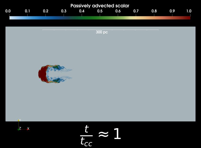
10 Kanjilal, Dutta, Sharma 2020
10 9 10 7 10 5 10 3 10 7 10 5 10 3 10 1
threshold for cloud growth depends on the time till which we look
Volume weighted PDF Volume weighted PDF
for such growth and this needs to be comparable to hot gas cooling
t 3tcc t 3tcc time. This may explain most of the apparent differences between
6.0
our and Gronke-Oh numerical results versus those of Sparre et al.
5.5 (2020).
The typical simulation domain chosen by Li et al. (2020a) is
log10(T[K])
5.0 smaller (20 × 10 × 10Rcl 3 ) than our fiducial box-size (400 × 30 ×
3
30Rcl ). For a small box and outflow boundary conditions (used in
4.5
the downstream longitudinal direction), the mixed/dense gas can
4.0 leak out of the simulation domain. Thus, small box simulations can
suppress the formation of cool gas seeds, which leave the simulation
box rather than seed the growth of cold gas in the long cloud tail.
t 6tcc t 6tcc Such a cold cloud would grow in larger boxes. We explore the effects
6.0
of the box-size and the boundary conditions in Appendix A. We
5.5 indeed verify that a smaller simulation box gives a larger threshold
radius for the growth of cold gas (the bottom panel of Figure A1)
log10(T[K])
5.0 but the effect just on its own is not big enough to explain the large
difference between the Gronke-Oh and Li radii. For example, a box-
4.5
size of (20, 10, 10)Rcl for Rcl /dcell = 8 shows cloud growth for the
4.0
cloud-size interpolation parameter β = 0.6 (β = 0.5 corresponds to
the geometric mean of Gronke-Oh and Li radii; see Eq. 6) whereas
our fiducial run (using a large box-size) with β = 0.5 shows growth.
t 12tcc t 12tcc The left panel of Figure 4 shows that in some of our simula-
6.0
tions, especially closer to the threshold radius for growth, there is a
5.5 significant dip in the cold mass at early times before the cloud starts
to grow. Moreover, in the left panel of Figure B1 we find that the
log10(T[K])
5.0 time till the dip in cold gas mass is longer for a higher resolution
with a larger dip in cold mass (Appendix B investigates the effect
4.5 of resolution). Note that Li et al. (2020a) use a mass resolution of
∼ 10−6 Mcl , which corresponds to Rcl /dcell ∼ 64 in the dense phase,
4.0
∼ 40( χ/100)−1/6 in the intermediate phase and ∼ 14( χ/100)−1/3
2.2 2.4 2.6 2.8 3.0 3.2 0 50 100 150 200 250 300 in the hot phase, much higher than our (and that of Sparre et al.
log10 kPB [Kcm 3]
( )
Relative Speed (kms 1) 2020) typical resolution Rcl /dcell = 8. The red line in the left panel
of Figure B1, which corresponds to Rcl /dcell = 64 and a box-size
Figure 7. The joint volume weighted probability distributions of pressure-
temperature (left panels) and relative speed-temperature (relative to the
of (30, 15, 15)Rcl , shows a dip in the dense mass fraction below
hot wind material; right panels) at different times for the fiducial run with 0.1. So the cloud in this run, according to the definition used by Li
Rcl /dcell = 8. From the top row to the bottom, the plots are made at {3,6,12} et al. (2020a), will be labelled as destroyed. Since the box-size of
tcc . The pressure does not exhibit a lot of variation, especially at late times, Li et al. (2020a) is even smaller ([20, 10, 10]Rcl ) the drop in dense
indicating an approximate isobaric evolution. The hot wind starts to entrain mass fraction will be even more. Therefore, a combination of a high
the cold gas due to turbulent momentum transport by about a drag time resolution and a small box-size leads them to misidentify growing
∼ 10tcc , consistent with the right panel of Figure 4. The red crosses indicate clouds as destroyed.
the position of the peaks corresponding to the initial (t = 0) probability Apart from these factors, the mismatch in the simulation results
distribution. may be due to the difference between the numerical algorithms. Li
et al. (2020a) use the mesh-free smooth particle hydrodynamic
for higher χ and M also demands a larger box-size because the code GIZMO (Hopkins 2015) while Gronke & Oh (2018, 2020)
mixed gas has more time to leave the box through the downstream use a finite volume Godunov code ATHENA (Stone et al. 2008).
boundary. Generally fixed-grid codes overestimate numerical mixing, so they
Li et al. (2020a) declare a cloud destroyed when its mass falls are expected to give a larger threshold cloud radius than a moving
below 10% of its initial mass but the dense gas may still grow mesh or a mesh-free code. But our and Gronke-Oh simulations,
even after such a large dip. Very recently, Sparre et al. (2020) have based on fixed-grid codes, give a smaller threshold radius for the
performed numerical simulations of the cloud-crushing problem growth of cold gas than Li et al. (2020a) who use a mesh-free code!
with cooling (their resolution Rcl /dcell = 7 for χ = 100, similar to Thus a quantitative resolution of Gronke & Oh 2018 and Li et al.
ours) and mapped out the parameter regime for the growth of cold (2020a) results, and mapping out of the precise growth threshold
gas by monitoring the cold gas mass till 12.5tcc for most of their runs. require further work and a closer comparison.
However, the left panel of Figure 4 clearly shows that the growth 5 Caveats & future directions
of cold gas can occur after this time, especially for large density
While the discovery of a criterion for the growth of cold gas in
contrasts ( χ) and Mach numbers (M).?? Thus, the all-important
cooling turbulent boundary layers is an important milestone (Gronke
?? The top-right panel in Figure 8 of Sparre et al. (2020) shows that their
numerical results agree with the Gronke-Oh criterion for χ = 100 and a longer time, and the conclusions drawn from their simulations will not
M = 0.5. Some of their runs may show dense mass growth if analyzed for disagree much with ours.
MNRAS 000, 1–14 (2020)Multiphase gas in the cloud-crushing problem with cooling 11
102 102
& Oh 2018), there are several conundrums still remaining to be 100
1.5 t=0 t=0
101 t 6 tcc t 6 tcc 101
solved when applying this idea to the observations of the CGM and 1.4
( , , Rcl[pc]) 100 100
galactic outflows. Even before that, the exact threshold needs to be (50,1.0,6.79)
M(T < 3Tcl)/Mcl, 0
M > 3cl /Mcl, 0
M0 d(log10[T/Thot])
M0 d(log10[n/ncl])
mapped out with high resolution 3-D simulations of large enough 1.3 10 1 10 1
)
dM
dM
10 1
boxes. 1.2 10 2 10 2
(
The Gronke-Oh criterion is based on the implicit assump-
1
1
10 3 10 3
1.1
tion that the cooling function peaks at the intermediate tempera- 10 4 10 4
1.0
tures. Moreover, estimating the cooling time of the mixing layer as 0 1 2 3 4 5 6 7
10 5 10 5
(ThotTcl )1/2 is not rigorously justified. This important estimate will t 2.0 1.5 1.0 0.5 0.0
tcc log10(n/ncl) and log10(T/Thot)
clearly depend on the exact shape of the cooling function. The ef-
fective cooling function can be quite different, for example, in AGN Figure 8. The left: Figure shows the dense (ρ > ρcl /3; in red) and cold
outflows irradiated by intense radiation (Dyda et al. 2017). (T < 3Tcl ; in blue) mass fraction as a function of time (left panel) and the
In several multiphase media, the cooling time of the hot dif- mass PDFs of density (red) and temperature (blue) at t = 6tcc (right panel;
initial PDFs are shown by dotted lines) for the run with a density contrast
fuse phase is shorter than the timescales of interest; e.g., the inner
χ = 50 (see Table 3). The dense (ρ > ρcl /3) mass evolution in the left
CGM (e.g., Cavagnolo et al. 2009) and the central parts of galactic panel incorrectly suggests that the cloud much larger than the Gronke-Oh
outflows (e.g., Thompson et al. 2016). In this case most of the cold radius (≈ 1 pc; Eq. 3) is destroyed with time. On the other hand, the cold
gas can be produced by the cooling of the hot gas with large density (T < 3Tcl ) mass grows with time. This contrasting behavior is because of
perturbations (Choudhury et al. 2019) cooling in turbulent bound- cooling of the hot wind and the expansion of the dense cloud in presence
ary layers. The cloud-crushing studies assume a pre-existing dense of the reduced ambient pressure. The right: Figure shows the mass PDF
cloud, the origin of which is non-trivial. The cold gas can condense of density (normalized to ncl ) at 6tcc (in red) confirms that the peak cold
out of the hot CGM if the ratio of the cooling time to the free-fall density shifts to lower than ncl /3. The hot gas temperature peak (in blue)
time is less than a threshold . 20 (Voit et al. 2015; Lakhchaura et al. moves to < Thot /3, indicating a decrease in the confining pressure. The hot
2018). Cold clouds can be pushed up and entrained by superbubbles gas density and the cold gas temperature at 6tcc still peak at their initial
values.
√ Once again like before, the PDFs are associated with a spread ∝
blowing out of the gas disk (Vijayan et al. 2018; Schneider et al.
1/ bin count − 1.
2020) but they seem to get destroyed by ∼ 10 kpc, implying that the
cold gas growth in the turbulent boundary layers depend crucially
on the background conditions and is not yet fully understood. Ram
pressure stripped galactic wakes (e.g., Ebeling et al. 2014) are an- cold (< 3Tcl ) gas mass shows growth. How is it that the cold mass
other way to seed cool/dense gas that can cool and seed growing grows but the dense mass decreases? The reason is the cooling of
cold clouds (Tonnesen & Bryan 2010; Yun et al. 2019; Nelson et al. the background hot wind, which decreases the ambient temperature
2020). and pressure. In a low ambient pressure, the cold gas at ∼ 104 K
In the standard cloud-crushing problem, the cold gas eventually expands isothermally and reduces its density to ρ < ρcl /3 but the
becomes comoving and the turbulent cooling boundary layer does gas at T < 3Tcl keeps building up with time.
not exist any more. In order to quantitatively apply cloud-crushing The importance of the χ/M dependence of the hot wind cool-
results to CGM clouds, the background gravity must be taken into ing time and the appropriate time-window to analyze cloud growth
account. The question of the survival of the IGM filaments penetrat- in the boundary layer, presented as the key cause of discrepancy be-
ing into the CGM of halos of different masses (Dekel et al. 2009) tween the Gronke-Oh and Li criteria for cloud growth in section 4.5,
is also intimately connected to the interplay of turbulent boundary is reinforced by this example.
layers and cooling (Mandelker et al. 2020; Fielding et al. 2020).
Apart from the various issues discussed above, there are the 6 Summary
usual concerns about the convergence of numerical results in ab- In this paper, we systematically analyze the survival of cold gas in
sence of explicit dissipation (e.g., Koyama & Inutsuka 2004). Im- the cloud-crushing problem in presence of optically thin radiative
portant physical effects such as thermal conduction, magnetic fields, cooling, particularly for the parameters relevant to the CGM. Our
background turbulence (e.g., Mohapatra & Sharma 2019; Li et al. conclusions are summarized as follows:
2020b), and cosmic rays (e.g., Butsky et al. 2020) can definitely
affect the small scale structure of the multiphase plasma. This (i) We analyze the large discrepancy (see Figure 1) between the
rich problem clearly deserves to be studied systematically, care- cloud growth criteria predicted by Gronke & Oh (2018, 2020) and
fully benchmarking the effects of these various important effects. Li et al. (2020a). In our numerical simulations, clouds smaller than
Only after this can we confidently apply the cloud-crushing results the Li radius and larger than the Gronke-Oh radius show the growth
to the observed multiphase plasmas. of cold gas (see Figure 2). The main reason that Li et al. (2020a) see
cloud destruction for somewhat smaller clouds is the combination
5.1 Hot wind cooling time & cloud growth
of a small box-size and a very high resolution, combined with
As an example of caution that we need to exercise in order to apply their definition of cloud destruction. The principal reason of our
the cloud-crushing results, we consider the cloud-crushing problem discrepancy with Sparre et al. (2020) is perhaps that they do not run
with cooling for a density contrast of χ = 50. In this case, the their simulations long enough (see section 4.5). Simulations with
background cooling time is not much longer than the cooling time larger density contrast and Mach numbers should be run for more
of the mixed gas (see Figure 6). Figure 8 shows the dense (ρ > ρcl /3) cloud-crushing times because the cooling time of the hot wind is
and cold (T < 3Tcl ) mass evolution for a cloud at χ=50, M = 1.0, longer. Thus, our results stress the importance of the cooling time of
and a radius of Rcl ≈ 8RGO (see Eq. 3). From the left panel, we the mixed gas rather than the hot gas for the growth of dense mass.
can clearly see that the dense mass is destroyed after ≈ 6tcc , with However, more work is needed to map out the exact cloud growth
the evolution similar to the cases where clouds are destroyed due to threshold with large boxes and sufficient resolution. It is also unclear
inefficient cooling in the mixing layer. However, the evolution of the whether the most appropriate temperature of the mixing layer to
MNRAS 000, 1–14 (2020)You can also read