NSW Estuary Tidal
Inundation Exposure
Assessment
←
→
Page content transcription
If your browser does not render page correctly, please read the page content below
NSW Estuary Tidal Inundation Exposure Assessment
© 2018 State of NSW and Office of Environment and Heritage
With the exception of photographs, the State of NSW and Office of Environment and
Heritage are pleased to allow this material to be reproduced in whole or in part for
educational and non-commercial use, provided the meaning is unchanged and its source,
publisher and authorship are acknowledged. Specific permission is required for the
reproduction of photographs.
The Office of Environment and Heritage (OEH) has compiled this report in good faith,
exercising all due care and attention. No representation is made about the accuracy,
completeness or suitability of the information in this publication for any particular purpose.
OEH shall not be liable for any damage which may occur to any person or organisation
taking action or not on the basis of this publication. Readers should seek appropriate advice
when applying the information to their specific needs.
All content in this publication is owned by OEH and is protected by Crown Copyright, unless
credited otherwise. It is licensed under the Creative Commons Attribution 4.0 International
(CC BY 4.0), subject to the exemptions contained in the licence. The legal code for the
licence is available at Creative Commons.
OEH asserts the right to be attributed as author of the original material in the following
manner: © State of New South Wales and Office of Environment and Heritage 2018.
Acknowledgements
Funding for this study was provided by the Natural Disasters Resilience Program. Water
level data was kindly provided by Manly Hydraulics Laboratory. Terrain data was provided by
Land and Property Information (LPI), Coffs Harbour City Council, Tweed Shire Council and
Great Lakes Council. Many thanks to Dr John Church and Professor Bruce Thom for their
peer review of the report.

Published by:
Office of Environment and Heritage
59 Goulburn Street, Sydney NSW 2000
PO Box A290, Sydney South NSW 1232
Phone: +61 2 9995 5000 (switchboard)
Phone: 131 555 (environment information and publications requests)
Phone: 1300 361 967 (national parks, general environmental enquiries, and publications requests)
Fax: +61 2 9995 5999
TTY users: phone 133 677, then ask for 131 555
Speak and listen users: phone 1300 555 727, then ask for 131 555
Email: info@environment.nsw.gov.au
Website: www.environment.nsw.gov.au

Report pollution and environmental incidents
Environment Line: 131 555 (NSW only) or info@environment.nsw.gov.au
See also www.environment.nsw.gov.au

ISBN 978-1-76039-958-0
OEH 2017/0635
July 2018

Find out more about your environment at:

www.environment.nsw.gov.au

NSW Estuary Tidal Inundation Exposure Assessment

Contents
List of figures                                                           iv
List of tables                                                            vi
Executive summary                                                         vii
1.   Introduction                                                          1
     1.1 Context                                                           1
     1.2 Aim and scope of the assessment                                   2
2.   The NSW coast                                                         4
     2.1   Introduction                                                    4
     2.2   Regional setting and estuary types                              4
     2.3   Tidal characteristics                                           9
     2.4   Non-astronomic contributors to water levels                    12
3.   Sea level rise                                                       15
     3.1   Past sea level fluctuations                                    15
     3.2   Historical global mean sea level rise                          15
     3.3   Future sea level projections                                   18
     3.4   Land movement                                                  22
4.   Approach to the risk assessment                                      23
     4.1   Introduction                                                   23
     4.2   Tidal planes                                                   23
     4.3   Offshore tidal boundary conditions                             24
     4.4   Estuarine tidal plane evaluation                               28
     4.5   Terrain data                                                   34
     4.6   Inundation mapping                                             35
     4.7   Sea level rise scenarios                                       36
     4.8   Exposure assessment                                            36
5.   Results of the exposure assessment                                   40
     5.1 Introduction                                                     40
     5.2 Statewide exposure                                               40
     5.3 Regional exposure                                                46
6.   Findings                                                             66
     6.1 Summary                                                          66
     6.2 Limitations                                                      66
     6.3 Recommendations                                                  68
7.   References                                                           70
8.   Appendices                                                           76

                                              iii
NSW Estuary Tidal Inundation Exposure Assessment
List of figures
Figure 1.2.1. Tidal inundation of low-lying urban areas in Newcastle 14/12/2009
(photos: B Coates) 3
Figure 2.2.1. Characteristics of drowned river valleys (source: Roy et al. 2001) 6
Figure 2.2.2. Characteristics of young barrier estuaries (source: Roy et al. 2001) 7
Figure 2.2.3. Characteristics of mature barrier estuaries (source: Roy et al. 2001) 8
Figure 2.2.4. Characteristics of saline coastal lakes (source: Roy et al. 2001) 9
Figure 2.3.1. Tidal characteristics in different estuary types (source: NSW
Government 1992); note differences in scale 11
Figure 3.2.1. Global mean sea level from 1880 to 2012 16
Figure 3.2.2. Regional distribution of sea level trends from 1993 to 2011, based on
satellite altimeter data 17
Figure 3.2.3. Observed sea level trends from Jan. 1993 to Dec. 2011 in the
Australian region from satellite altimeter data (colour contours) and tide
gauges (coloured dots); both after correction for GIA 18
Figure 3.3.1 Projections of global mean SLR over the 21st century relative to 1986–
2005, for RCP2.6 and RCP8.5 20
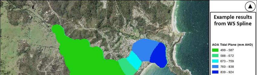
Figure 3.3.2. (a) Percentage of the deviation of the ensemble mean net regional sea
level change between 1986–2005 and 2081–2100 from the global mean
value; (b) Total RCP4. 5 sea level change (plus all other components)
divided by the combined standard error of all components 21
Figure 4.3.1. Map of NSW showing location of MHL tide gauges 25
Figure 4.3.2. Plot of tidal range R for NSW extracted from OTIS model; map is on
Universal Transverse Mercator (UTM) projection 26
Figure 4.3.3. Plots showing comparison between HHWSS values from OTIS and
data for open ocean locations (named in blue) and onshore open ocean
gauging locations (named in black) 27
Figure 4.3.4. Along coast variation in extreme (100 year ARI) water level and
HHWSS for open ocean (named in blue) and onshore open ocean gauging
locations (named in black) 28
Figure 4.4.1. Examples of tidal planes for different estuary types: (a) Drowned River
Valley (Hawkesbury River), (b) Large River (Clarence River), (c) Small
River (Merimbula Lake), (d) Tidal Lake (Lake Illawarra), HHWSS in red,
MSL in blue and ISLW in green 30
Figure 4.4.2. Plot showing categorisation of NSW estuary types using high water
entrance gradient and length of estuary 32
Figure 4.4.3. Average HHWSS tidal plane for different estuary types: (a) Drowned
River Valley, (b) Large River, (c) Small River, and (d) Tidal Lakes 33
Figure 4.6.1. Flowchart showing simplified structure of GIS-based Water Surface
Model and Inundation Model 35
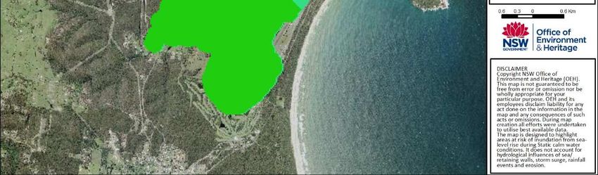
Figure 4.6.2. Plot showing example results of WS-spline tool from the Water Surface
Model 36
iv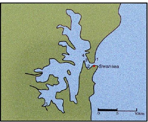
NSW Estuary Tidal Inundation Exposure Assessment

Figure 4.8.1. Procedure used to identify valid address types for the coastal
          inundation exposure assessment (source: OEH 2014)                      38
Figure 5.2.1. (a) Total numbers of properties exposed to inundation (HHWSS) for all
          NSW estuaries under 0, 0.5, 1.0 and 1.5 m SLR; (b) As for (a) but including
          percentage-of-lot inundated                                            41
Figure 5.2.2. (a) Total numbers of properties exposed to inundation (100 year ARI
          water levels assuming HHWSS plus 0.5 m for DRV, LR, SR, TL – but
          excluding ICOLLs where berm height was used) for all NSW estuaries
          under 0, 0.5 and 1.0 m SLR; (b) As for (a) but including percentage-of-lot
          inundated                                                               42
Figure 5.2.3. Total numbers of properties exposed to inundation (HHWSS) for the 10
          most exposed NSW estuaries under 0, 0.5, 1.0 and 1.5 m SLR           43
Figure 5.2.4. Total numbers of properties exposed to inundation (HHWSS) for the 10
          most exposed NSW estuaries, including proportion-of-lot, under 0, 0.5, 1.0
          and 1.5 m SLR                                                          43
Figure 5.2.5. (a) Kilometres of roads exposed and (b) Kilometres of roads including
          breakdown of road type for all NSW estuaries under 0, 0.5, 1.0 and 1.5 m
          SLR                                                                     44
Figure 5.2.6. (a) Kilometres of power lines exposed and (b) Kilometres of power lines
          including breakdown of power line type for all NSW estuaries under 0, 0.5,
          1.0 and 1.5 m SLR                                                       45
Figure 5.2.7. (a) Kilometres of railways exposed and (b) numbers of airfields exposed
          for all NSW estuaries under 0, 0.5, 1.0 and 1.5 m SLR                   45
Figure 5.3.1. Map showing boundaries of NSW planning regions                     46
Figure 5.3.2. (a) Total numbers of properties exposed to inundation (HHWSS) for
          each region under 0, 0.5, 1.0 and 1.5 m SLR; (b) As for (a) but including
          percentage-of-lot inundated                                             47
Figure 5.3.3. (a)Total numbers of properties exposed to inundation (100 year ARI
          water levels assuming HHWSS plus 0.5 m for DRV, LR, SR, TL – but
          excluding ICOLLs where berm height was used) for each region under 0,
          0.5 and 1.0 m SLR; (b) As for (a) but including percentage-of-lot inundated
                                                                                  48
Figure 5.3.4. (a) Kilometres of roads exposed and (b) Kilometres of roads including
          breakdown of road type for each region, under 0, 0.5, 1.0 and 1.5 m SLR
                                                                                  50
Figure 5.3.5. (a) Kilometres of railways exposed and (b) Kilometres of railways
          including breakdown of railway type for each region, under 0, 0.5, 1.0 and
          1.5 m SLR                                                               51
Figure 5.3.6. (a) Kilometres of power lines exposed and (b) Kilometres of power lines
          including breakdown of power line type for each region, under 0, 0.5, 1.0
          and 1.5 m SLR                                                           52
Figure 5.3.7. Total numbers of properties exposed to inundation (HHWSS) for the 10
          most exposed estuaries in the North Coast region under 0, 0.5, 1.0 and 1.5
          m SLR: (a) Number of properties affected; (b) Percentage of each property
          affected                                                              55

                                              v
NSW Estuary Tidal Inundation Exposure Assessment

Figure 5.3.8. Total numbers of properties exposed to inundation (HHWSS) for the
          seven estuaries in the Hunter region under 0, 0.5, 1.0 and 1.5 m SLR: (a)
          Number of properties affected; (b) Percentage of each property affected
                                                                                 57
Figure 5.3.9. Total numbers of properties exposed to inundation (HHWSS) for the
          eight estuaries in the Central Coast region under 0, 0.5, 1.0 and 1.5 m
          SLR: (a) Number of properties affected; (b) Percentage of each property
          affected                                                                59
Figure 5.3.10.       Total numbers of properties exposed to inundation (HHWSS) for
          the 10 most exposed estuaries in the Metropolitan Sydney region under 0,
          0.5, 1.0 and 1.5 m SLR: (a) Number of properties affected; (b) Percentage
          of each property affected                                              61
Figure 5.3.11.      Total numbers of properties exposed to inundation (HHWSS) for
          the 10 most exposed estuaries in the Illawarra region under 0, 0.5, 1.0 and
          1.5 m SLR: (a) Number of properties affected; (b) Percentage of each
          property affected                                                       63
Figure 5.3.12.      Total numbers of properties exposed to inundation (HHWSS) for
          the 10 most exposed estuaries in the South East and Tablelands region
          under 0, 0.5, 1.0 and 1.5 m SLR: (a) Number of properties affected; (b)
          Percentage of each property affected                                    65

List of tables
Table 2.2.1. Types of water bodies in eastern Australia (source: after Roy et al.
          2001)                                                                   5
Table 4.2.1. Major constituents used in tidal plane calculations (MHL 2012)      23
Table 4.8.1. Proportion-of-lot inundation categories used to differentiate between
          different levels of exposure                                            39
Table 5.2.1. Number of properties statewide exposed to inundation (HHWSS) on a
          proportion-of-lot basis                                           41
Table 5.2.2. Number of properties statewide exposed to inundation (100 year ARI
          water levels) on a proportion-of-lot basis                          42
Table 5.3.1. GURAS database and inundation modelling statistics of properties
          affected for each NSW planning region                               47
Table 5.3.2. GURAS database and inundation modelling statistics of properties
          affected (≈100 year ARI) for each NSW planning region               49
Table 5.3.3. GURAS database and inundation modelling statistics of roads affected
          for each NSW planning region                                         52
Table 5.3.4. GURAS database and inundation modelling statistics of railway affected
          for each NSW planning region                                         53
Table 5.3.5. GURAS database and inundation modelling statistics of power lines
          affected for each NSW planning region                                53

                                             vi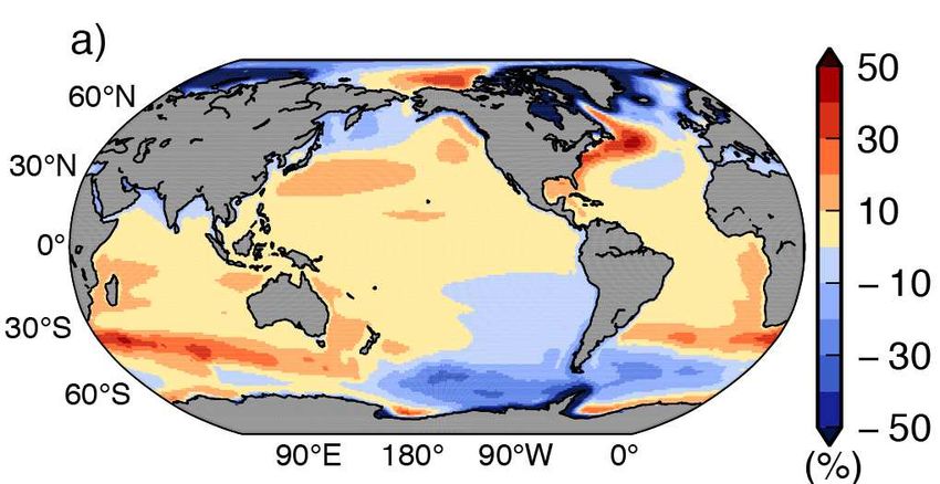
NSW Estuary Tidal Inundation Exposure Assessment

Executive summary
Key findings
Communities and infrastructure along the coast of New South Wales are highly vulnerable to
climate change. In this study, we assess exposure of current development to inundation
associated with a range of potential, future sea level rise (SLR) scenarios.
Results show that 23,653 properties are exposed to tidal inundation (at the High High Water
Solstice Springs level) if sea level rises by 0.5 m (metres), 50,744 if sea level rises by 1 m
and 74,379 with 1.5 m of SLR.
On a proportion-of-lot basis the analysis shows many properties are only subject to minor
inundation, although as sea levels increase the proportion of properties subject to major or
complete inundation increases. Numbers of properties subject to greater than 50%
inundation are 4186 for 0.5 m of SLR, 21,582 for 1 m of SLR and 42,950 for 1.5 m of SLR.
Numbers of properties subject to greater than 90% inundation are 1,620 for 0.5 m of SLR,
13,456 for 1 m of SLR, and 33,104 for 1.5 m of SLR.
Allowing for storm surge and other non-tidal contributors to ocean water levels (≈100 year
annual return interval (ARI)), 51,557 properties are exposed to ocean inundation if sea level
rises by 0.5 m, and 74,746 if sea level rises by 1 m. Numbers of properties subject to greater
than 50% inundation are 20,263 for 0.5 m of SLR and 40,607 for 1 m of SLR. The number of
properties subject to greater than 90% inundation is 15,061 for 0.5 m of SLR and 33,789 for
1 m of SLR.
Greatest exposure occurs around tidal lakes and adjacent to the large and more heavily
populated coastal river systems. Within tidal lakes, reduced tidal range in combination with
extensive coastal flats has allowed development to occur in relative proximity to sea level.
For coastal rivers, exposure is associated with the extensive nature of the tidal rivers on the
north coast and with high levels of development in the Sydney region.
Using state planning regions, greatest exposure occurs in the North Coast region,
contributing to around 31.5% of the statewide exposure across all scenarios. This is followed
by the Metropolitan Sydney region with 22% of the statewide exposure. High levels of
exposure are also found in the Hunter and Central Coast regions. Lowest exposure is found
in the Illawarra and the South East and Tablelands regions with 7.5% and 3% of statewide
exposure respectively.
On a proportion-of-area basis, the Central Coast region is the most exposed in the state and
Lake Macquarie is the most exposed individual estuary. Overall the Hunter and Central
Coast regions contribute 18% each to the statewide exposure across all scenarios. Here
extensive development has occurred on the low-lying areas adjacent to the coastal lake
systems.

Context
Global mean sea levels are rising and this is expected to continue for centuries, even if
greenhouse gas emissions are curbed and their atmospheric concentrations stabilised.
The United Nations Intergovernmental Panel on Climate Change fifth assessment (IPCC
2013) projections indicate global mean sea level rise under a business-as-usual scenario
(RCP8.5) of between 0.52 m and 0.98 m, by 2100 relative to 1986–2005 or 0.28 m and 0.61
m with significant reduced emissions (RCP2.6). The rate of SLR over the 21st century is
projected to very likely exceed recently observed rates of SLR. For business-as-usual
emissions (RCP8.5) projected rates of SLR reach 8–16 mm (millimetres) per year by the end
of the century. With significantly reduced emissions (RCP2.6) the projected rate of rise

                                                vii
NSW Estuary Tidal Inundation Exposure Assessment

becomes roughly constant (central projection about 4.5 mm per year) before the middle of
the century, and subsequently declines slightly.
SLR is not uniformly distributed and most coastlines around the world are projected to
experience sea level change within about 20% of the global average. For New South Wales,
mean model predictions suggest SLR of 0–10% above the global average (Church et al.
2013).
Beyond 2100 the IPCC (2013) conclude that it is virtually certain that global mean SLR will
continue for many centuries due to thermal expansion of the oceans and melting glaciers and
ice sheets. Assuming lowest emission scenarios, modelling indicates global mean SLR
above the pre-industrial level by 2300 will be less than one metre, however for higher
emissions the projected rise is one metre to more than three metres. These models likely
underestimate the Antarctic ice sheet contribution, resulting in an underestimate of projected
SLR beyond 2100.
The IPCC (2013) predict warming greater than a threshold above 1°C but less than about
4°C would lead to the near-complete loss of the Greenland ice sheet. This would result in a
global mean SLR of up to seven metres over a millennium or more. They also suggest abrupt
and irreversible ice loss from a potential instability of marine-based sectors of the Antarctic
ice sheet in response to climate forcing is possible, but current evidence and understanding
is insufficient to make a quantitative assessment.

Approach
In this study, we assess exposure to current development from inundation associated with a
range of SLR scenarios. We focus on risk in estuaries, largely because these areas have
considerable development in relatively close proximity to sea level, while the open coast is
characterised by dunes that provide some level of protection against inundation. We exclude
erosion, which will be addressed in a separate study.
We focus on exposure to tidal inundation at the High High Water Solstice Springs (HHWSS)
level and or berm height in mostly closed coastal lakes and lagoons. The HHWSS tidal plane
is consistent with levels for higher (king) tides. At ocean tide gauge sites, this level is
exceeded on average 25 days a year due to contributions from non-tidal processes including
storm surge, coastal trapped waves, etc. SLR scenarios of 0.5 m, 1.0 m and 1.5 m are
assessed. The use of a 0.5 m water level offset also allows a first order estimation of effects
of less frequent inundation at around the 100-year annual return level associated with storm
surge and other non-tidal processes (excluding wave setup, runup and riverine flooding
effects).
The study uses a mid-level approach to the modelling and mapping of water levels within
estuaries. The approach adopted is based on measured tidal plane data and allows for
variation in tidal levels both between and along estuaries. The method thus improves on
simple bathtub type approaches used in previous assessments.
We utilise tide gauge data for 56 estuaries (MHL 2012) for current estuarine water levels.
This data is also used to categorise NSW estuary planes and identify characteristic tidal
plane types for application to non-gauged estuaries.
The water surface mapping methodology adopted uses an interpolated tidal plane created
from gauge data or berm heights for mostly closed lakes and lagoons. Tidal planes are
overlain on digital elevation models derived from high resolution data. The resulting spatial
model of inundation greatly improves the representation of current inundation hazard areas
and allows for improved assessment of the inundation hazard associated with potential SLR.
Inundation mapping is undertaken and the extents are used to quantify risk based on data
from the Geocoded Urban and Rural Addressing System (GURAS) database. The degree of
inundation is examined through quantification of the proportion of each lot inundated.

                                               viii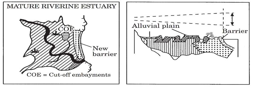
NSW Estuary Tidal Inundation Exposure Assessment

Limitations
The assessment of exposure is underpinned by a number of assumptions and limitations
related to available data. The approach adopted, while allowing for variation in water levels
between and along individual estuaries, still remains a broadscale assessment. It does not
replace the need to undertake flood or inundation studies for individual estuaries and results
should not be used to assess risk to individual properties and assets.
The study adopts the HHWSS tidal plane and or berm heights for water surface mapping.
This tidal plane is slightly lower than highest astronomical tide (HAT) and thus does not
represent the full extent of tidal inundation. Additionally, this tidal plane does not include non-
tidal processes including storm surge, although the 0.5 m sea level offset may also be
representative of a first order allowance for 100-year ARI non-tidal water level variations.
However, this excludes effects of wave setup, runup and coincident rainfall-related flooding.
The tidal planes fitted within estuaries should be considered approximate only. Within
gauged estuaries the planes are limited by the availability of data and the accuracy of the
formulations used to calculate the plane. In ungauged estuaries, we adopt planes from
gauged estuaries of the same estuary type, thus assuming average conditions by type.
Estimated accuracies of average tidal planes for each estuary type are: Drowned River
Valleys ±0.06 m, Large Rivers ±0.11 m, Small Rivers ±0.15 m and Tidal Lakes ±0.10 m.
Three scenarios are considered: SLRs of 0.5 m, 1 m and 1.5 m. These are selected to be
representative of a range of future sea levels relevant to structure design as well as land-use
planning. They are not tied to particular planning horizons and importantly should not be
considered an upper bound for potential long-term SLR which may need to be considered for
future development.
SLRs are added to the existing tidal planes and thus assume no change in tidal range or
form. Inundation extents are mapped by overlying tidal plane surfaces on digital elevation
models derived from LiDAR data, which have a vertical accuracy of around 0.3 m. The
exposure assessments assume geomorphology remains unchanged with future sea level
except within ICOLLs (intermittently closed and open coastal lake or lagoons) where an
increase in berm height is applied.
Exposure is quantified using data from the GURAS database. Major limitations associated
with this relate to the fact that an exposed address may not equate to an exposed asset, as
asset elevation is not considered. The exposure assessment is limited to broadscale
quantification of the inundation of property and infrastructure. Many impacts on the
environment and ecosystem services are also likely with SLR, but these have not been
considered in this assessment.

Recommendations
This assessment shows a considerable amount of development along the NSW coast is at
risk from SLR. The assessment highlights the importance of, and need for, coastal zone and
floodplain management planning to manage risk to current development and to avoid
unnecessary expansion of risk in the future.
In relation to coastal risk management we recommend:
   •   review of existing coastal zone and/or floodplain management plans and their
       adequacy for managing risks associated with SLR
   •   preparation or update of coastal zone and/or floodplain management plans as
       required to manage current and potential future risk
   •   implementation of these plans to reduce current and potential future exposure to SLR

                                                 ix
NSW Estuary Tidal Inundation Exposure Assessment

   •   management using risk management principles which consider likelihood (and
       uncertainty) and hazard with a focus on solutions that are flexible and robust
   •   adoption of strategies that address the ongoing nature of SLR (beyond 2100),
       including measures to avoid the expansion of development in areas likely to be
       subject to future inundation or alternatively, adoption of measures that recognise the
       temporary nature of such areas (temporary occupancy)
   •   education concerning SLR and coastal processes and hazards
   •   mapping and assessment of actual (built) and planned/potential (land-use zoning) risk
       exposure at regular intervals (5–10 years) for a prescribed set of sea level scenarios.
In relation to improvement of risk assessment techniques we recommend:
   •   further research on open coast hazards including wave runup on beaches and
       coastal erosion
   •   further research on potential morphodynamic changes to coastal systems associated
       with SLR. This should include effects of potential changes to entrance configuration
       and marine delta sedimentation on tidal processes in different estuary types, as well
       as foreshore erosion/accretion and wetland response
   •   further research on impacts of SLR on rainfall-related flooding and coincident events.

                                               x
NSW Estuary Tidal Inundation Exposure Assessment
1. Introduction
1.1 Context
Global mean sea levels are rising and this rise is expected to continue for centuries, even if
greenhouse gas emissions are curbed and their atmospheric concentrations stabilised. As
global temperature increases, rising ocean heat content causes ocean thermal expansion
and sea level rise. Other contributions to sea level rise come from the melting of land ice,
including glaciers and ice caps, as well as the major ice sheets of Antarctica and Greenland.
Around the Australian coast sea levels are also rising. Rates of rise here are generally
thought to be consistent with the global average, with a recent review finding the Australian
average rate of relative sea level rise (SLR) between 1966 and 2009 was 2.1 ± 0.2 mm per
year and from 1993 to 2009 the rate was 3.1 ± 0.6 mm per year (White et al. 2014).
The United Nations Intergovernmental Panel on Climate Change (IPCC) projections indicate
global mean sea mean level rise under a business-as-usual scenario (RCP8.5) of between
0.52 m and 0.98 m by 2100, relative to 1986–2005, or 0.28 m and 0.61 m with significantly
reduced emissions (RCP2.6) (IPCC 2013). The rate of SLR over the 21st century is projected
to very likely exceed recently observed rates of SLR. For business-as-usual emissions
(RCP8.5) projected rates of SLR reach 8 to 16 mm per year by the end of the century. With
significantly reduced emissions (RCP2.6) the projected rate of rise becomes roughly
constant (central projection about 4.5 mm per year) before the middle of the century, and
subsequently declines slightly.
SLR is not uniformly distributed and most coastlines around the world are projected to
experience sea level change within about 20% of the global average. For New South Wales,
mean model predictions suggest SLR of 0–10% above the global average (Church et al.
2013 Figure 13.21).
Beyond 2100 the IPCC (2013) conclude that it is virtually certain that global mean SLR will
continue for many centuries due to thermal expansion of the oceans. Assuming lower
emission scenarios, global mean SLR above the pre-industrial level by 2300 will be less than
one metre; however, this significantly increases for higher emissions as the projected rise is
from one metre to more than three metres. These models likely underestimate the Antarctic
ice sheet contribution, resulting in an underestimate of projected SLR beyond 2100.
Sustained warming greater than a threshold above 1°C (low confidence) but less than about
4°C (medium confidence) would lead to the near-complete loss of the Greenland ice sheet
over a millennium or more, causing a global mean SLR of up to seven metres. Abrupt and
irreversible ice loss from a potential instability of marine-based sectors of the Antarctic ice
sheet in response to climate forcing is possible, but current evidence and understanding is
insufficient to make a quantitative assessment.
Communities in Australia are considered highly vulnerable to SLR. Chen and McAneney
(2006) estimate that approximately 711,000 addresses in Australia are located within three
kilometres of the shore and in areas below six metres above sea level, and over 60% of
those addresses are in Queensland and New South Wales. This analysis also found that the
majority of addresses are adjacent to lakes, lagoons, rivers and estuaries, rather than the
open ocean.
The National Coastal Vulnerability Assessment (DCC 2009; DCCEE 2011; Cechet et al.
2011, 2012) further refined the above estimate to identify between 157,000 and 247,600
existing residential buildings in Australia at risk of inundation with a sea level rise of 1.1 m. In
NSW between 40,800 and 62,400 residential buildings were identified as being at risk from
the combined effect of 1.1 m of SLR and a 100-year annual return period storm tide.
1NSW Estuary Tidal Inundation Exposure Assessment
Incorporating commercial addresses brings the total exposure to between 41,550 and
63,650 (Cechet et al. 2012).
The impacts of SLR are likely to include the erosion of sandy beaches and the increased
frequency, depth and extent of coastal flooding. Increased ocean water levels during storms
are virtually certain to result in more frequent coastal inundation, higher wave runup levels,
higher water levels in lakes and estuaries and more flooding in coastal rivers. This suite of
changes will have a progressively increasing impact on existing low-lying coastal
development.
Developments along the NSW coast that are near current high tide levels will be susceptible
to more frequent tidal and ocean inundation. Additionally, as sea levels rise, stormwater
drainage is likely to become less effective, impacting urban areas near coastal rivers, lakes
and estuaries. Communities currently susceptible to the combined effects of marine and
catchment flooding will be further affected with SLR; the scale of impacts will vary dependent
on the vulnerability of each location.
Dunes on the open coast tend to be elevated significantly above sea level and thus provide
some level of protection against inundation (but are subject to erosion). Estuarine areas are
typically characterised by extensive low-lying areas however, often with considerable
development in relatively close proximity to sea level. It is these areas that are the focus of
the current investigation.
1.2 Aim and scope of the assessment
In this study, we undertake a statewide assessment of the impact of inundation in estuaries
associated with projected SLR on the NSW coast. The aim of the study is to refine estimates
of the extent of current exposure of properties and infrastructure to potential SLR to help
assess the need for, and prioritisation of, adaptation planning and action.
The study focuses on risk to development surrounding estuary foreshores. This is because
considerable development is located in low-lying areas adjacent to estuarine foreshores and
is potentially vulnerable to inundation. In many areas, inundation of low-lying streets and
foreshores occurs now and highlights potential vulnerability to SLR (see Figure 1.2.1). On
the open coast, beaches tend to be backed by relatively high dunes and bounded by
headlands. Historically inundation of these areas has not been a major concern except at
isolated locations (although erosion is a major concern). Wave setup and runup play a
significant role in inundation on the open coast with measured runup heights on steep,
exposed beaches during storms exceeding 7 m. (PWD 1988; Nielsen & Hanslow 1991).
Assessment of wave setup and wave runup requires detailed modelling which is beyond the
scope of the current study. We exclude erosion, which will be addressed in separate study.
2NSW Estuary Tidal Inundation Exposure Assessment
Figure 1.2.1. Tidal inundation of low-lying urban areas in Newcastle 14/12/2009 (photos: B
Coates)
We focus on exposure to tidal inundation at the High High Water Solstice Springs (HHWSS)
level although our approach also allows first order assessment of less frequent ocean
inundation at around the 100-year annual return level (excluding wave setup, runup and
coincident catchment flooding). The study uses a mid-level approach to the modelling and
mapping of water levels within estuaries. The method adopted is based on measured tidal
plane data which allows for variation in tidal levels both between and along estuaries, and
thus improves on simple bathtub type approaches used in previous assessments (e.g. DCC
2009).
Tides along the NSW coast are semi-diurnal with a significant diurnal equality, and tidal
range varies along the coast increasing from south to north. Tidal levels in estuaries vary
depending on estuary type, with some systems exhibiting tidal amplification while others
display significant attenuation compared with ocean tidal levels (NSW Government 1992;
Druery et al. 1983).
Interpolated tidal planes are created from gauge data and mapped tidal limits and applied in
conjunction with high resolution elevation data. The resulting spatial model of inundation
greatly improves the representation of current inundation hazard areas and allows for
improved assessment of the inundation hazard associated with potential SLR.
Data from the Geocoded Urban and Rural Addressing System (GURAS) are used to identify
and quantify properties that are predicted to be exposed to inundation under SLR scenarios
of 0.5 m, 1.0 m and 1.5 m.
The exposure assessment is limited to broadscale quantification inundation to property and
infrastructure. Many impacts on the environment and ecosystem services are also likely with
SLR but these have not been considered in this assessment. Other exclusions include the
effects of wave setup and runup and coincident catchment flooding. While all these effects
are likely to be important, their assessment requires work which was beyond the scope of
this assessment
3NSW Estuary Tidal Inundation Exposure Assessment
2. The NSW coast
2.1 Introduction
The NSW coast stretches for some 1590 kilometres from the Queensland border to the
Victorian border (Short 2007). The coast is exposed to the predominant south east swell and
experiences a moderate to high energy wave regime. The shoreline is comprised of areas of
rocky cliffs and headlands joined by sandy beaches (Chapman et al. 1982).
On the coast south of Sydney, the beaches are predominantly pocket beaches isolated by
rocky headlands with little alongshore sand exchange from compartment to compartment. In
the north of the state, these beaches tend to be longer and alongshore rates of sand
movement are higher, with sand moving from compartment to compartment, predominantly
from south to north. Beaches are typically backed by high dunes which provide some
protection against storm surge and wave inundation but experience episodic erosion.
There are approximately 184 significant estuaries along the NSW coast. These vary
significantly in shape and size, ranging from large coastal embayments and drowned river
valleys, such as the Hawkesbury River, to coastal lakes, such as Lake Macquarie and Wallis
Lake, and smaller intermittently open coastal lakes and lagoons, such as Manly Lagoon and
Tabourie Lake (NSW Government 1992; Roper et al. 2011). Estuaries support many
different habitat types and species, highly valued by local communities.
In many estuaries, considerable development is located on the low-lying land immediately
adjacent to foreshores and much of this is prone to occasional inundation, both as a result of
storm and floods but also simply as a result of high ocean levels and/or prevailing entrance
conditions. For many estuaries, the entrances are managed to reduce this flooding risk
either through permanent structures (breakwaters and training walls), or in the smaller lakes,
through the artificial opening of the entrances by local councils to control water levels (NSW
Government 1992).
2.2 Regional setting and estuary types
The present character of the NSW coast is the result of multiple phases of sea level
fluctuation over millions of years. Over this time, the bedrock valleys in which estuaries lie
have been gradually infilled with marine and terrestrial sediment. During periods of SLR, vast
quantities of marine sand were reworked and transported landward as transgressing sand
sheets and barriers. In many locations along the NSW coast, separate barriers can be
recognised, corresponding to cycles of sea level variation.
The onshore transport of this marine sand enclosed rivers and estuaries. These vary in
character depending on the degree of barrier formation and the nature of the inherited
coastal topography (Roy & Thom 1981; Roy 1984).
As sea level approached present day mean sea level, extensive sand barriers were formed
across the mouths of broad, shallow embayments. Landward of these barriers, estuaries
were created in the form of broad tidal lakes connected to the ocean by narrow tidal inlets
through the barrier.
Deep narrow mouthed embayments, such as Port Jackson and the Hawkesbury–Broken
Bay System, led to a different form of estuary evolution. The transgressing sand sheets were
unable to completely fill the mouths of deep embayments before sea level stabilised. The
incipient barriers remained submerged and the estuaries developed as drowned river valleys
with wide mouths which extended across the width of the embayment.
Roy et al. (2001) classify eastern Australian coastal water bodies into a range of groups and
types based on the degree of marine influence. These estuary groups include: bays, tide
4NSW Estuary Tidal Inundation Exposure Assessment
dominated estuaries, wave dominated estuaries, intermittent estuaries and freshwater
bodies (Table 2.2.1).
Table 2.2.1. Types of water bodies in eastern Australia (source: after Roy et al. 2001)
Estuary group Type Mature form
Bays Ocean embayments
Funnel shaped macro tidal
estuaries
Tide dominated estuaries Tidal estuaries
Drowned river valley estuaries
Tidal basins
Barrier estuaries
Wave dominated estuaries Barrier lagoons Riverine estuaries
Interbarrier estuaries
Saline coastal lagoons
Intermittent estuaries Small coastal creeks Saline creeks
Evaporative lagoons
Brackish barrier lakes
Freshwater bodies Perched dune lakes Terrestrial swamps
Backswamps
The main estuary types found in NSW are drowned river valleys, barrier estuaries and
coastal lakes.
2.2.1 Drowned river valley estuaries
Drowned river valley estuaries are easily recognisable because of their wide bedrock-flanked
mouths, the presence of a submerged flood tidal delta and the absence of a sub-aerial sand
barrier at their entrances (NSW Government 1992). Examples include the Hawkesbury River
and Sydney Harbour. The basic form of the drowned river valley is a steep sided bedrock
valley which deepens and widens in the seawards direction. Upper catchment sediments
typically reclaim the upstream reaches of drowned river valleys, which today consist of
extensive floodplains with tidal river channels. Downstream of these areas, the size and
depth of the relict drowned valley is dependent upon the dimensions of the parent valley and
the relative sediment supply from the upper catchment. For instance, in Port Hacking, which
has only a small upper catchment and therefore a relatively low sediment yield, there is a
difference of 30 metres in depth between the upper fluvial delta (formed from terrestrial
sediments) and the shoals of the submerged tidal delta at the entrance (formed from marine
sediments).
5NSW Estuary Tidal Inundation Exposure Assessment
Figure 2.2.1. Characteristics of drowned river valleys (source: Roy et al. 2001)
2.2.2 Barrier estuaries
Young barrier estuaries exist as tidal lakes. They are characterised by relatively small upper
catchments. Consequently, the sedimentation that has occurred since sea levels stabilised
has not been sufficient to infill the initial back barrier lake.
The shape, depth and size of the tidal lakes are variable depending on the size of the parent
embayment and the rates of sediment supply from the catchment. They vary from very small
systems like Narrabeen Lagoon to Lake Macquarie, the largest tidal lake in Australia (see
Figure 2.2.2).
6NSW Estuary Tidal Inundation Exposure Assessment
Figure 2.2.2. Characteristics of young barrier estuaries (source: Roy et al. 2001)
Mature barrier estuaries have been created by extensive river systems with relatively high
sediment loads. The high sediment loads have infilled the initial back barrier lake with
alluvium, causing the development of sinuous river channels discharging directly into the
ocean (tidal rivers). Contiguous floodplains with backwater swamps and cut-off bays are
vague reminders of the former back barrier lakes.
Mature barrier estuaries range in size from large systems like the Clarence, Richmond and
Hunter rivers to small systems like Coffs, Bonville and Currumbene creeks (see Figure
2.2.3).
7NSW Estuary Tidal Inundation Exposure Assessment
Figure 2.2.3. Characteristics of mature barrier estuaries (source: Roy et al. 2001)
2.2.3 Saline coastal lagoons/intermittently closed and open lakes and
lagoons
Saline coastal lagoons are small systems which have intermittent entrances that are closed
to the ocean for most of the time (NSW Government 1992). These have become known as
intermittently closed and open lakes and lagoons (ICOLLs) (Haines et al. 2006). Under
natural conditions, the ocean entrance opens only when a large build-up of catchment runoff
breaches the beach berm. Saline coastal lakes comprise mostly small systems such as Dee
Why and Manly lagoons, but they can include larger systems such as Wollumboola Lake
(see Figure 2.2.4).
8NSW Estuary Tidal Inundation Exposure Assessment
Figure 2.2.4. Characteristics of saline coastal lakes (source: Roy et al. 2001)
2.3 Tidal characteristics
2.3.1 Ocean tides
Tides along the NSW coastline are semi-diurnal in nature, i.e. high water and low water
occur about twice daily (the actual period of a tidal cycle is about 12.5 hours). They are
sinusoidal in shape and have a pronounced diurnal inequality (successive high tides differ
markedly).
The mean spring range is 1.2 m while the mean neap range is 0.8 m (AHO 2011; MHL
2012). The mean range at Sydney is 1.0 m, with mean high water of 0.52 m AHD (Australian
Height Datum) and mean low water of –0.48 m AHD (MHL 2012). Tidal range varies slightly
along the coast with an increase of around 0.2 m from south to north (MHL 2011).
2.3.2 Tides within estuaries
The rise and fall of ocean water levels travels along an estuary as a long wave. The speed of
travel or celerity of this wave varies with water depth; the deeper the water, the faster the
wave celerity.
As the tide propagates into the shallow waters of an estuary it is subject to a number of
changes (NSW Government 1992). These include:
• Tidal lag – the delay between a standard state of the tide at the estuary mouth,
such as high tide, and the occurrence of the same state of tide inside the
estuary.
9NSW Estuary Tidal Inundation Exposure Assessment
• Tidal distortion – relates to the shape of the tidal wave as it moves landward.
It occurs because the speed of propagation of the tide at high water is faster
than at low water. As a consequence, the tide rises faster than it falls and peak
flood tide velocities are generally greater than peak ebb tide velocities.
• Elevation of half-tide levels or tidal pumping – the higher celerity of the
flood tide compared to the ebb tide results in a tendency for greater upstream
movement of water on the flood tide compared to downstream movement on
the ebb tide. This leads to a dynamic trapping of water in the upper reaches of
the estuary, as reflected in a super-elevation of half-tide level. Elevated half-
tide levels act to increase the seaward flow of water and so provide an overall
flow balance.
• Amplification of fortnightly tides – this is thought to be related to the trapping
of water in the upstream reaches of an estuary. Variation in the volume of
trapped water during the fortnightly spring–neap tide cycle can produce a
significant fortnightly variation in half-tide level (the fortnightly tide). This effect
is particularly noticeable in large coastal lakes.
The tidal range in estuaries is affected by several processes (Dyer 1997; McDowell &
O’Connor 1977; Savenije 2005; Prandle 2009; Van Rijn 2010), including:
• inertia related to acceleration and deceleration effects
• amplification associated with the decrease of the width and depth (convergence)
• attenuation due to bottom friction particularly across the flood tidal delta
• partial reflection at abrupt changes of the cross-section and at the landward end
of the estuary (in the absence of a river).
These processes result in fundamentally different patterns of tidal behaviour in different
estuaries. Some estuaries experience tidal amplification while others are characterised by
tidal attenuation (Van Rijn 2010). In New South Wales differences in tidal behaviour within
estuaries have been recognised for some time (Roy & Thom 1981; Druery et al. 1983; Roy
1984, NSW Government 1992; MHL 1995a, b; MHL 2002; MHL 2003; MHL 2005; MHL
2012).
NSW Government (1992) describes the tidal behaviour of NSW estuaries on the basis of
estuary shapes which generally correspond to the estuary types described above. However,
different estuary types can, in some instances, share similar tidal behaviour; for example,
mature barrier estuaries, such as the Hunter River, display similar tidal behaviour to a
mature drowned river valley estuary, such as the Karuah River, probably because the
entrance bar and delta complex has been dredged to allow for port activities.
The main estuary shapes influencing tidal behaviour are as follows:
Drowned river valley estuaries – The younger stages of drowned river valley estuaries are
characterised by channels which generally deepen and widen in the seawards direction. The
landward narrowing of the channel promotes tidal amplification through the concentration of
flow. As the channel shallows, tidal resonance also helps to maintain a high tidal range.
River valley estuaries display no initial attenuation but often exhibit amplification of the ocean
tidal range.
In such estuaries, the tidal range is only attenuated in the upstream reaches where the
cumulative dissipative effects of bed friction dampen tidal flows. For example, amplification
occurs over most of the length of the Hawkesbury River, with the tidal range at Wisemans
Ferry, which is approximately midway along the estuary, 16% greater than the ocean range.
10NSW Estuary Tidal Inundation Exposure Assessment
The tidal range at Windsor, which is 123 kilometres upstream from the estuary mouth, is
slightly less than ocean range. Upstream of Windsor, the presence of coarse shallow sand
shoals abruptly reduces tidal range to 26% of the ocean value (NSW Government 1992)
(see Figure 2.3.1a).
a. Drowned river valleys
b. Barrier estuaries
c. Coastal lakes
Figure 2.3.1. Tidal characteristics in different estuary types (source: NSW Government
1992); note differences in scale
River estuaries (mature barrier estuaries) – Tidal rivers in New South Wales are
characterised by relatively narrow and shallow entrance channels of relatively constant width
and constant depth, consisting predominantly of sandy bed sediments. They include the
mature stages of barrier estuaries and drowned river valley estuaries.
The shallow nature of the channels promotes tidal resonance which is counter-balanced by
energy losses across entrance shoals and frictional dissipation at the sandy bed.
Consequently, the tidal range along the estuary nearly always displays initial attenuation,
followed by mild amplification before complete damping at fluvial gravel and sand bars
around the head of the estuary (NSW Government 1992).
This behaviour is illustrated by the Manning River (see Figure 2.3.1b). At Manning Point,
only three kilometres upstream from the estuary mouth, the tidal range is only 50% of the
ocean value (because of the dissipative effects of the entrance bar).
11NSW Estuary Tidal Inundation Exposure Assessment
In these systems, some long-term morphodynamic variation in tidal range can occur with
changing entrance shoals (MHL 2012).
Tidal lakes (young barrier estuaries) – Tidal lakes are characterised by a broad expanse
of tidal water, connected to the ocean by a relatively small tidal channel, referred to as a tidal
inlet (see Figure 2.3.1c). The depth of water in the lake is always greater than that of the
inlet. They show severe attenuation of the tidal range due to frictional effects in the entrance
channel. Tide ranges in these systems may be as little as 10% of that offshore and tidal
pumping can significantly amplify the magnitude of the fortnightly tide (McLean & Hinwood
2011).
Nielsen and Gordon (2011) show several tidal lake systems in New South Wales are
undergoing long-term morphodynamic adjustment following the installation of river entrance
training walls, including ongoing increases in tide range and discharge as a result of
entrance scour and increasing entrance efficiency. Examples include Lake Macquarie, Wallis
Lake and Lake Illawarra.
Intermittently closed and open lakes and lagoons (ICOLLs) – Smaller lake systems are
usually characterised by intermittent entrance opening and closing. While open they operate
like tidal lakes, while closed they gradually fill with water levels influenced by inflows and
evaporation (Haines et al. 2006).
In these systems, maximum water levels are generally controlled by beach berm height
(Hanslow et al. 2000; Haines 2006). Berms are wave built features and result from the
onshore transport of sand. Berm height is dependent on wave runup which in turn is
controlled by wave height and period and beach slope or grain size (Hanslow et al. 2000;
Weir et al. 2006).
2.4 Non-astronomic contributors to water levels
Variations in water level due to non-astronomic factors (i.e. factors not included in tidal
predictions) are common along the NSW coast and are associated with a range of
oceanographic and meteorological processes. MHL (1992) shows that anomalies of 0.3 m
occur at return intervals of months, and thus become a significant addition to tidal
predictions. Drivers of tidal anomalies include variations in air pressure and wind stress
which during storms is known as ‘storm surge’; coastal trapped waves; ocean currents; steric
effects; seiches; tsunamis; Rossby waves, etc. At gauges located in riverine settings they
can also include effects of freshwater flow (flooding). These processes operate over a wide
range of time frames.
Studies of the Fort Denison tide record show inter-annual and multi-decadal variability linked
with both the El Niño Southern Oscillation (ENSO) and the Interdecadal Pacific Oscillation
(IPO) (Holbrook et al. 2010; MHL 2011). These oscillations see variation in annual mean sea
level of around 10 centimetres. At higher frequencies, many factors contribute to anomalies
but the largest are associated with storm surge and/or coastal trapped waves (CTWs).
CTWs are large-scale waves which propagate along continental margins. They have long
wave lengths (around 2000 kilometres) and periods (around 10–20 days) and are generated
by weather disturbances. The majority of CTWs have been shown to propagate as
continuous features between south Western Australia and north eastern Australia although
some CTWs on the east coast are also generated by strong winds in Bass Strait. They have
average wave heights of around 0.2 m, sometimes up to 0.5 m, and can elevate coastal
water levels for several days (SMEC & UQ 2013; Church et al. 1986a, b; Maiwa et al. 2010,
Woodham et al. 2013). Larger CTWs are generally thought to be associated with
reinforcement by strong wind forcing on the southern part of the east coast and/or Bass
Strait. It is likely that the large size of one particular CTW was a result of ongoing
reinforcement associated with the series of frontal systems that impacted southern Victoria
and Bass Strait over the second week of May.
12NSW Estuary Tidal Inundation Exposure Assessment Storm surge (the combined effect of reduced air pressure and wind setup), while smaller than on many coasts worldwide, can still raise water levels along Australia’s east coast by over 50 centimetres above normal (e.g. NSW Government 1992). In NSW, the duration of storm surges varies from short-lived events of less than a day to several days depending on storm characteristics and propagation. Annual anomalies increase slightly from south to north along the NSW coast (MHL 2011). Storm surge is usually the largest single contributor to tidal anomalies and extreme ocean levels; however, joint coincidence with other drivers also needs to be considered. Within river entrances water depth and entrance morphology play a significant role both in modifying tidal behaviour and in wave breaking, which may influence mean water levels through wave setup. These effects are likely to vary significantly between different estuary types. Wave setup on beaches results in significant super-elevation of mean water levels particularly near the beach face, however water depths in most river entrances are likely to mean wave setup is significantly lower than on beaches (Hanslow & Nielsen 1992). Measurements from the Brunswick River entrance in northern NSW suggest wave setup is minor within moderate sized trained river entrances (e.g. Nielsen & Hanslow 1995; Hanslow et al. 1996). Examination of extreme value distributions by You et al. (2012) has similarly demonstrated limited evidence of wave setup in trained river entrances in New South Wales. They show reduced extreme water levels at the trained river entrances compared with offshore sites and suggest this is likely due to the attenuation in tidal range through the river entrances. It is probable that the trained entrance water depths in these systems are too deep to generate significant wave setup. Additionally, the presence of training walls, which extend into the surf zone, may introduce a physical barrier to higher mean water levels from wave setup on the neighbouring sandy beaches (Hanslow & Nielsen 1992). You et al. (2012) highlight however that their results may not be applicable to smaller coastal systems (e.g. lagoons or creeks) where water depths may become shallow enough to allow wave setup or in untrained river systems where there is no physical barrier between the beach/swash zone and the entrance. Most smaller, estuarine systems tend to be only intermittently open to the sea and thus berm heights become important for determining extreme water levels (Haines 2006). With climate change, there are numerous potential changes to non-astronomic water level drivers including both oceanographic processes and those associated with catchment- related flooding; for example, changes to the intensity of storms and storm surge and changes to oceanographic processes associated with the warming and strengthening of the East Australian Current. The magnitude and likelihood of these changes however, remains uncertain. McInnes et al. (2007) show only minor changes to storm surge with climate change for Wooli and Batemans Bay on the north and south coasts of New South Wales respectively. Wave modelling by Hemer et al. (2012) suggests a minor decrease in mean significant wave height (
NSW Estuary Tidal Inundation Exposure Assessment

2.4.1 Joint coincidence with catchment flooding
Storm surge-related tidal anomalies may be generated by weather phenomena that also
contribute to coastal rainfall and potentially flooding, thus considerations concerning joint
coincidence become more important. For these events however, numerous questions need
to be examined. These concern the:
    •   influence of ocean conditions on the tidal waterway
    •   relative scale of coastal and catchment flooding events
    •   relative timing of peak rainfall and flood relative to the peak of ocean conditions
    •   type of storm cell (synoptic type) that is likely to lead to significant catchment
        flooding and/or significant coastal flooding and whether they correspond
    •   importance of the catchment size, shape and available waterway volume
    •   relative location of the community in relation to the waterway and its entrance.
Several studies have identified the synoptic storm types critical to the generation of extreme
wave and water level conditions along the NSW coast (Shand et al. 2011; Blain, Bremner
and Williams 1985). These appear to have much in common with those identified as
contributing to heavy rain events (e.g. Speer et al. 2009). Speer et al. (2009) note that
systems that develop within subtropical easterly wind regimes, namely inland trough lows
and easterly trough lows, account for 71% of the significant rain events and when combined
with the ex-tropical cyclone category, account for 84% of the heavy rain events. These types
also make up a significant proportion of the synoptic types resulting in wave heights over five
metres along the NSW coast (Shand et al. 2011).
Recent preliminary studies on joint coincidence of rainfall and ocean events suggest some
coincidence, particularly where catchment and coastal flooding are both being driven by the
same synoptic type (McPherson et al. 2012). The exact nature of the coincidence of coastal
and catchment flooding is likely to vary with estuary type and size.

                                               14
NSW Estuary Tidal Inundation Exposure Assessment
3. Sea level rise
3.1 Past sea level fluctuations
Sea level is not static but has undergone numerous fluctuations throughout geological
history. Over the last two million years there have been 30–40 major oscillations in sea level,
some in excess of 120 metres (Imbrie et al. 1984; Lowe & Walker 1984; Peltier 1999). These
oscillations have had a significant influence on the evolution of the coastal zone we know
today, and are responsible for the complex array of beach barrier and estuary systems which
make up the current coastline.
These fluctuations are thought to be initiated by the orbital motions of the Earth and result in
major shifts in climate between glacial and interglacial phases. As the Earth orbits around
the sun and spins around its axis, several quasi-periodic variations occur. These oscillations,
known as Milankovitch cycles, relate to the Earth’s eccentricity, obliquity and precession.
They change the amount and location of solar radiation reaching the Earth and have a
significant influence on long-term climate. Once initiated, these variations lead to positive
feedback with greenhouse gases in the atmosphere, promoting major climatic shifts.
The last full interglacial/glacial cycle occurred over the last 125,000 years and has seen sea
levels fluctuate by 120 metres. The cessation of the last glacial phase resulted in a global
rise in sea level from levels around 120 metres below current sea level to its present level.
This rise began about 18,000 years ago with sea levels approaching their current levels
around 7000–8000 years ago.
Relative sea level records from sites around the world however, show great diversity in the
maximum height reached and in the timing of the peaks. The causes for these regional
variations is a complex interaction of geomorphic and geological controls including
tectonism, climate, sediment discharge and/or compaction, tidal changes, local geoid
perturbations and isostatic warping. Regionally and even locally these factors create vertical
changes in the elevation of the ground, thus offsetting or enhancing changes in sea level.
In south eastern Australia, recent compilations of geomorphic evidence for sea level change
over the last 10,000 years include those undertaken by Lewis et al. (2012) and Sloss et al.
(2007). This suggests sea level reached its current level around 7000–8000 years ago. This
work shows that for much of the last 7000 years relative sea level has been slightly above
present levels. There has however, continued to be much debate about the exact timing of
when sea level reached its current level and whether a Holocene highstand occurred (see
Murray-Wallace & Woodroffe 2014 for summary).
3.2 Historical global mean sea level rise
Church and White (2011) use monthly sea level data from the Permanent Service for Mean
Sea Level (PSMSL; Woodworth & Player 2003) and satellite altimeter data to show that
between 1880 and 2009 the global average sea level increased by about 210 mm (Figure
3.2.1). Rhein et al. (2013) determine that it is very likely that the average rate of mean SLR
was 1.7 ± 0.2 mm per year between 1901 and 2010 and that this rate increased to 3.2 ±
0.4 mm per year between 1993 and 2010.
3.2.1 Regional distribution of sea level rise
While global mean SLR is relatively consistent, there are significant regional variations
throughout the ocean basins of the world. These are attributable to variations in the
distribution of thermal expansion, local and regional meteorological effects, ocean
circulation, and regional responses to modes of climate variability; for example, the ENSO
and the Pacific Decadal Oscillation (PDO).
15You can also read