P-Ride: A Shareability Prediction Based Framework in Ridesharing
←
→
Page content transcription
If your browser does not render page correctly, please read the page content below

electronics
Article
P-Ride: A Shareability Prediction Based Framework
in Ridesharing
Yu Chen               and Liping Wang *

                                          School of Software Engineering, East China Normal University, Shanghai 200062, China; yu.chen@stu.ecnu.edu.cn
                                          * Correspondence: lipingwang@sei.ecnu.edu.cn

                                          Abstract: Ridesharing services aim to reduce travel costs for users and optimize revenue for drivers
                                          and platforms by sharing available seats. Existing works can be roughly classified into two types,
                                          i.e., online-based and batch-based methods. The former mainly focuses on responding quickly to the
                                          requests, and the latter focuses on meticulously enumerating request combinations to improve service
                                          quality. However, online-based methods perform poorly in service quality due to the neglect of the
                                          sharing relationship between requests, while batch-based methods fail in terms of efficiency. To obtain
                                          better service quality more efficiently, we propose a shareability prediction-based framework P-Ride.
                                          Specifically, we first introduce the k-clique listing strategy in graph theory based on the shareability
                                          graph to reduce the infeasible request combinations. Moreover, we extend the shareability graph
                                          to the hypergraph structure to represent the higher-order shareable relationships among requests.
                                          Furthermore, we devise a shareability prediction model that supports the prediction of sharable
                                          relationships for request combinations of an arbitrary size, which helps further filtering of candidate
                                          request combinations with GPU devices acceleration. The extensive experimental results demonstrate
                                          the efficiency and effectiveness of our proposed P-Ride framework.

                                          Keywords: ridesharing; shareability graph; shareability prediction; intelligent transportation


Citation: Chen, Y.; Wang, L. P-Ride:
A Shareability Prediction Based           1. Introduction
Framework in Ridesharing.                      With the rapid development of the mobile internet and the sharing economy, rideshar-
Electronics 2022, 11, 1164. https://      ing has become an important transportation mode for traveling. In ridesharing services,
doi.org/10.3390/electronics11071164
                                          passengers share the available seats in vehicles in exchange for discounts on fees, while
Academic Editor: Felipe Jiménez           drivers and platforms realize higher revenues by improving the utilization of vehicles.
                                          Therefore, existing ridesharing service providers (e.g., Didi [1] and Uber [2]) are constantly
Received: 15 March 2022
                                          striving for improvements in service quality, such as higher platform service rates [3,4],
Accepted: 31 March 2022
                                          higher revenue [5,6] and reduced driving costs [5–8].
Published: 6 April 2022
                                               The ridesharing problem mainly focuses on the following two issues: request-vehicle
Publisher’s Note: MDPI stays neutral      matching and route planning. The existing works in solving the ridesharing problem can
with regard to jurisdictional claims in   be roughly classified into two categories: online-based [7–10] and batch-based [11–14]
published maps and institutional affil-   methods. For the request-vehicle matching problem, the online-based methods select the
iations.                                  vehicle with the lowest service cost for each request, according to a first-come, first-served
                                          strategy, and assign the request to the current best vehicle immediately, while the batch-
                                          based approaches meticulously group the requests in various combinations based on the
                                          strategy of grouping before the assignment and then select the appropriate vehicle for each
Copyright: © 2022 by the authors.
                                          group and assign the entire group of requests at once. For the problem of path planning,
Licensee MDPI, Basel, Switzerland.
                                          the insertion [9,10,13,15,16] method has been widely adopted in online-based methods. The
This article is an open access article
                                          insertion method updates the route by inserting the source and destination of the request
distributed under the terms and
conditions of the Creative Commons
                                          into the proper location of the vehicle’s current traveling route. Due to the insertion of
Attribution (CC BY) license (https://
                                          the source and destination of the insertion method without reordering the original route
creativecommons.org/licenses/by/          waypoints of the vehicle, the route obtained by the insertion method only provides a locally
4.0/).                                    optimal solution. In contrast, the batch-based method enumerates all feasible travel routes

Electronics 2022, 11, 1164. https://doi.org/10.3390/electronics11071164                                   https://www.mdpi.com/journal/electronics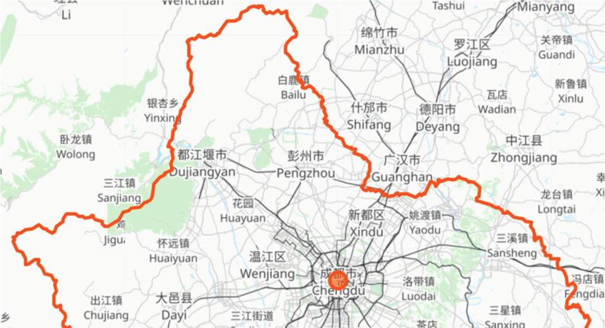
Electronics 2022, 11, 1164                                                                                                        2 of 18

                             for each request group and selects the best one for assignment to the service vehicle. In
                             general, the batch-based methods have better service quality (e.g., lower service cost, higher
                             service rate) because the online-based methods lack the analysis of shareable relationships
                             between requests and the detailed enumeration of routes, but the online-based methods
                             win in terms of efficiency.
                                   In this paper, we optimize the online-based method for the lack of shareable relation-
                             ship analysis between requests, and the batch-based method, which takes substantial time
                             for request group and optimal route enumeration. If there is a feasible route that can serve
                             two requests simultaneously, then we say that the two requests are shareable. We obtain
                             the structure of the shareability graph by adding an edge between all shareable requests
                             as nodes. In this paper, through the analysis of the sharability graph, we find that the
                             request group Q enumerated by the batch-based method inevitably forms a k-clique in the
                             sharability graph, i.e., all requests in Q hold an edge in the sharability graph. Additionally,
                             k-clique listing [17–19] is a well-studied classical problem in graph theory, based on the
                             observation that we can improve its performance by combining the efficient k-clique listing
                             algorithms available in graph theory with the batch-based approaches since the shareability
                             graph represented by the classical graph structure can only express the shareable relations
                             between binary requests, while the shareable relations between requests can often reach
                             more than three or four in practical applications. Therefore, we extend the shareability
                             graph to a hypergraph data structure to express multiple shareable relationships. Based on
                             the shareability hypergraph, we propose a shareable prediction model for predicting multi-
                             variate shareable relationships. The shareability prediction model predicts the shareable
                             relationships among multiple online requests simultaneously in fixed time based on the
                             historical shareable relationships among requests from different regions. The shareability
                             prediction model can significantly reduce the number of request groups enumerated in the
                             batch-based approach and save the computational cost.
                                   We will illustrate the motivation of this paper by the following example.

                             Example 1. In the ridesharing example shown in Figure 1a, there are four requests r1 . . . r4 with a
                             road network consisting of seven nodes a . . . g. The value close to each edge indicates the distance
                             between the connected two nodes. The details of the requests are shown in Table 1, where the release
                             time represents the time of the request submitted to the platform, and the deadline indicates the
                             expected arrival time to the destination. Suppose that the platform only allows one vehicle to service
                             up to two requests in a trip, and it takes one unit of time to move one unit of distance in the road
                             network. From the information given above, we have that r1 can share with r2 and r3 , and r2 can
                             share with r1 and r3 . However, r4 can only share with r2 . We can construct a shareability graph of
                             these four requests as shown in Figure 1b, where each edge indicates that the connected two requests
                             are shareable.
                                   Once the platform makes an allocation based on the online framework [7,8,16] (i.e., each request
                             will be served or discarded as soon as it arrives), it will choose requests r1 and r2 to share a vehicle,
                             which leads to the fact that requests r3 and r4 cannot share with other requests anymore when
                             they arrive.
                                   In the platform that adopts a batch-based framework [11–14], all possible request groups will be
                             checked and the optimal one will be taken into service. Through observing the shareability graph, we
                             found that the shareable requests are connected to each other. For example, request r1 cannot be shared
                             with r4 . Therefore, we can efficiently prune all request groups that contain r1 and r4 simultaneously
                             during the request group enumeration. Nevertheless, we still need to check the shareability of
                             request groups {r1 , r2 }, {r1 , r3 }, {r2 , r3 }, {r2 , r4 } and {r1 , r2 , r3 }. With the hypergraph-based
                             shareability prediction model proposed in this paper, we can predict the shareability of these request
                             groups simultaneously in a fixed time, which significantly improves the computational cost of the
                             batch-based methods.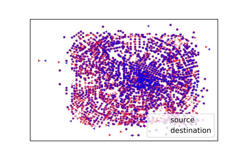
Electronics 2022, 11, 1164                                                                                                 3 of 18

                             Table 1. Requests release detail.

                                     Request               Source            Destination   Release Time            Deadline
                                          r1                 a                    d                0                  14
                                          r2                 c                    f                0                  11
                                          r3                 b                    e                2                  10
                                          r4                 c                    g                3                   9

                                                   +             &     2.3        (
                                                   #             2.3
                                                                                                            !
                                      $         1.4
                                                                 '
                                                                              7
                                 *

                                                %                        )
                                                                                             #              "              $
                                               !       "

                                               (a) Example Road Network.                         (b) Shareability Graph.

                             Figure 1. A motivation example.

                                     We summarize the main contributions of this paper as follows.
                             •       We study the dynamic ridesharing problem and optimize the efficiency of batch-
                                     based methods.
                             •       We propose a request group enumeration strategy based on k-clique listing on the
                                     shareability graph to optimize request group enumeration for batch-based methods.
                             •       We devise the P-Ride ridesharing framework with a shareability prediction model that
                                     supports the batch prediction of shareable relationships among a arbitrary number of
                                     requests in a fixed time.
                             •       Through extensive experiments, we demonstrate that the proposed method in this
                                     paper can significantly reduce the computational cost of batch-based methods. The
                                     P-Ride framework proposed in this paper can significantly improve efficiency with
                                     little impact on service quality.

                             2. Literature Review
                                   The ridesharing problem can be reduced to a variant of the Dial-a-Ride (DARP) prob-
                             lem [20,21], aiming to plan the vehicle routes and trip schedules for n requests who specific
                             source and destination with practical constraints. The existing works on ridesharing
                             services are categorized as static and dynamic, depending on whether all requests are
                             known in advance. Most of the existing works [22,23] on DARP are in a static environ-
                             ment. For the dynamic ridesharing problem, the existing solutions are mainly in online
                             mode [7,8,15,16] or batch mode [11–13,24].
                                   In online mode, insertion [25] is the state-of-the-art operation of the existing works [26,27]
                             in route planning, which inserts the pickup and drop-off locations of a new request into the
                             vehicle’s schedule without reordering. Tong et al. [16] proposed an insertion method based
                             on dynamic programming, which checks the constraints in constant time and dispatches
                             requests in linear time. Huang et al. proposed the structure of a kinetic tree in [8] to
                             trace all feasible routes for each vehicle to reduce the total drive distance. The kinetic tree
                             always provides the optimal vehicle schedule whenever the schedule changes (i.e., a new
                             request arrives).
                                   Batch-based algorithms partition the requests into groups and assign groups to their
                             appropriate vehicles. Alonso-Mora et al. [11] proposed an RTV-Graph to model the
                             relationship and constraints among requests, trips, and vehicles, where trips are the groups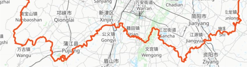
Electronics 2022, 11, 1164                                                                                                        4 of 18

                             composed of shareable requests. The RTV-Graph minimizes the utility function by linear
                             programming to allocate between vehicles and trips. The time cost for enumerating
                             trips in building RTV-Graph grows exponentially. Zeng et al. [12] proposed an index
                             called additive tree for pruning the infeasible groups during the group enumeration and
                             greedily chose the most profitable request group for each vehicle. Although the batch-
                             based methods achieve better service quality by meticulously enumerating request groups
                             compared to the online-based methods, the violent enumeration of request groups by
                             batch methods requires significant computational cost. Therefore, the ridesharing problem
                             critically requires an efficient way to analyze request shareable relationships and identify
                             the shareable request groups.
                                   The structure of the shareability graph adopted in this paper is intuitive, and thus some
                             similar structures have been used in some existing works, which are designed in different
                             ways for request-vehicle matching. Wang et al. [28] formulate a tree cover problem to serve
                             urban demands with as few vehicles as possible. Alonso-Mora et al. [11] optimally assign
                             vehicles to shareable groups of customers through linear programming. Zhang et al. [29]
                             formulate the passenger matching as a monopartite matching problem and solve it by the
                             Irving-Tan algorithm. However, the existing works based on sharability networks mainly
                             present sharable relationships through traditional graph structures, and traditional graphs
                             can only represent binary shareability relations among requests. However, in the rideshar-
                             ing scenario, the shareable relationship between requests often contains three or even more
                             requests, which cannot be properly represented in the existing shareability graphs.
                                   Therefore, in this paper, we propose the concept of the shareability hypergraph to
                             represent the high-order sharable relationship among requests, and we devise the share-
                             ability prediction model to identify shareable request groups of arbitrary size based on the
                             shareability hypergraph for fast screening of the shareable request groups.

                             3. Preliminary
                                  In this section, we introduce and analyze the dynamic ridesharing problem studied
                             in this paper. We used a directed weighted graph to represent the road network, where
                             each node in the graph represents an intersection and each edge indicates the road be-
                             tween intersections. Besides, each edge in the graph is associated with a weight cost(u, v),
                             which indicates the cost to travel from u to v. In this paper, cost(u, v) shows the average
                             travel time.

                             3.1. Definitions

                             Definition 1 (Request). Let ri = hsi , ei , ni , ti , di i denote an online request ri released at time ti ,
                             which contains ni passengers departing from si and requires one to arrive at ei before the deadline di .

                                  For each vehicle v j , it may be assigned with several numbers of mutually available
                             requests R j simultaneously. Therefore, we also need to plan a route S j for each vehicle v j ,
                             which consists of a sequence of pickup and drop-off locations for the requests r ∈ R j . We
                             define the route for each vehicle as follows.

                             Definition 2 (Route). Given a set of m requests R, let S = ho1 , ..., o2m i denote the route where o x
                             is the source location si or destination ei of request ri ∈ R.

                                  We mark a route as feasible if and only if it satisfies the following three constraints:
                             •    Sequential constraint. The pickup location si of request ri ∈ Ri should be located
                                  before the drop-off location ei in the feasible route.
                             •    Capacity constraint. At any location o x ∈ S, the total number of requests on the
                                  vehicle should not exceed the capacity of the vehicle.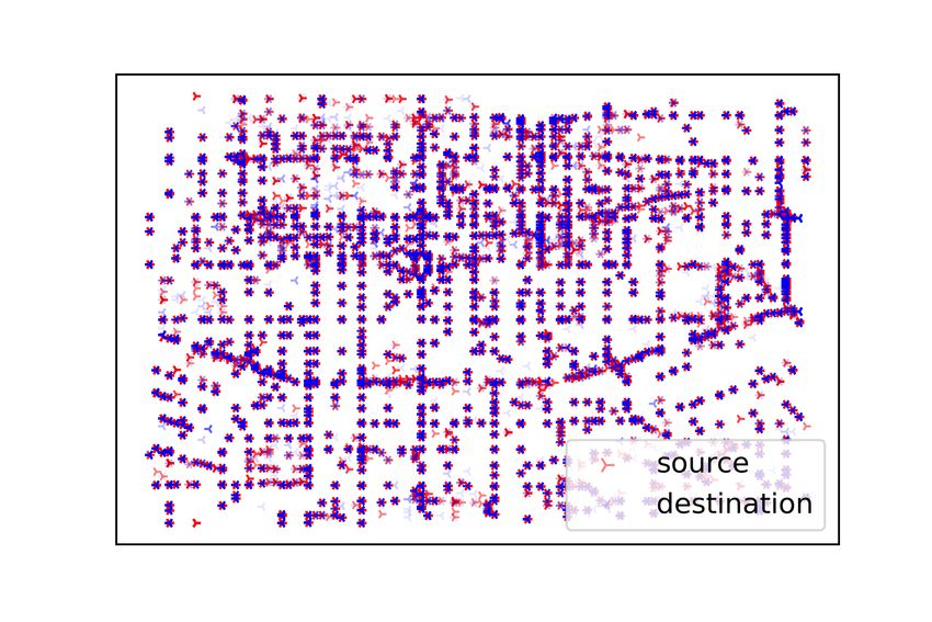
Electronics 2022, 11, 1164                                                                                                        5 of 18

                             •    Deadline constraint. For any location o x ∈ S, ∑kx=1 cost(ok−1 , ok ) ≤ ddl (ok ), where
                                  ddl (ok ) satisfied following Equation (1) for different location type (source or destination).
                                                                       (
                                                                         ei − cost(si , ei ), if o x is source
                                                           ddl (ok ) =                                                        (1)
                                                                         ei ,                      otherwise

                             Definition 3 (Shareable). Given a pair of requests r a and rb , we call it shareable if and only if
                             there exists a feasible route S for serving r a and rb simultaneously.

                                   We can extend the concept of sharable to multiple requests, i.e., we call the requests in
                             a set R sharable if there exists a feasible route that can serve all requests r ∈ R at the same
                             time. With the definitions above, we define the Dynamic Ridesharing Problem as follows.

                             Definition 4 (Dynamic Ridesharing Problem). Given a set R of n online requests and a vehicle
                             set W with maximum capacity constraint c, the Dynamic Ridesharing Problem requires planning a
                             feasible route for each vehicle w ∈ W to serve r ∈ R, which minimizes a specific utility function.

                                  In this paper, we refer to the following unified cost UC defined in [16] as the optimiza-
                             tion utility function. Specifically, the unified cost adopts the evaluation of total revenue
                             in [16], and the varying penalty coefficient β is equivalent to the balance between income
                             per unit time and fare per unit distance.

                                                     UC ( R, w) = α    ∑       µ ( S wi ) + β     ∑        cost(si , ei )            (2)
                                                                      w i ∈W                    ri ∈ R −

                                                              µ ( Sw ) =       ∑       cost(o x−1 , o x )                            (3)
                                                                           o x ∈ Swi

                                  Table 2 summarizes the commonly used symbols.

                             Table 2. Symbols and Descriptions.

                                                 Symbol                                                         Description
                                                    R                                    a set of m time-constrained request requests
                                                    ri                                           request request ri of request i
                                                    Sj                                          the planned route for vehicle v j
                                                    Q                                    a candidate request group with size | Q| ≤ c

                             3.2. Hardness of Dynamic Ridesharing Problem
                                  Following Theorem 1, we have that the dynamic shared travel problem is NP-Hard
                             and therefore intractable. Moreover, Tong et al. proved that there is no polynomial-time
                             algorithm with a constant competitive ratio for dynamic ridesharing problem [16].

                             Theorem 1 (Hardness of the Dynamic Ridesharing Problem). The Dynamic Ridesharing
                             Problem defined in Definition 4 is NP-hard.

                             Proof. We prove the theorem by a reduction from the URR problem defined in [9], which
                             has been proved to be an NP-hard problem. The URR problem can be briefly described
                             as follows: given a set R of m requests and a set V of n vehicles, each request is associated
                             with a source location si , a destination ei , a pickup deadline rti− and a drop off deadline
                             rti+ . The URR problem arranges requests to vehicles to maximize the utility function u with
                             capacity and time constraints.
                                    For a given URR problem, we can transform it into an instance of the BDRP problem:
                             we partition the requests ri ∈ R into a single element set Gi ; the route of Gi is a simple
                             shortest path from si to ei . In addition, we set the utility value for each vehicle and
                             group pairs as µ0 (v j , Gv j ) = −µ(v j , ri ). Then, for this BDRP instance, we would like to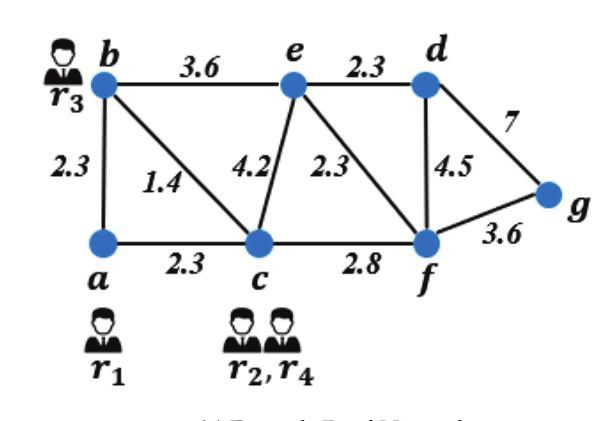
Electronics 2022, 11, 1164                                                                                              6 of 18

                             arrange a request group for the given vehicle with a route such that the summation utility
                             value ∑v j ∈V −µ0 (v j , Gv j ) is minimized. This shows that the URR problem can be solved in
                             polynomial time if and only if the transformed BDRP can be solved.
                                  In this way, we can reduce the URR problem to the BDRP. Since the URR problem
                             has been proved to be NP-hard, BDRP is also NP-hard. This completes the proof of
                             the theorem.

                             3.3. Brute-Force Solution
                                  The existing batch-based methods [11–14] for the Dynamic Ridesharing Problem are
                             based on a two-phase framework: (1) the enumeration of shareable request groups among
                             the request in each batch; (2) the matching between request groups and vehicles to minimize
                             the utility function. We summarize the batch-based methods as shown in Algorithm 1.

                             Algorithm 1 Brute-Force Solution
                             Require: A set R of n requests, a set W of m vehicles and a batch period τ
                             Ensure: The planned routes set S for vehicle w ∈ W
                              1: t ← current timestamp;
                              2: for every time period τ do
                              3:   R− ← {ri |ti ∈ [t, t + τ )}
                              4:   for w j ∈ W do
                              5:      G ← initialize a empty set for candidate shareable groups;
                              6:      for k ∈ [1..c] do
                              7:          G 0 ← enumerate shareable request groups g among R− where | g| = k;
                              8:          G ← G ∪ G0 ;
                              9:      end for
                             10:      g∗ ← ming∈G UC ( g, w);
                             11:      S ← enumerating routes for serving r ∈ g∗ ;
                             12:      S j ← arg minS∈S µ(S)
                             13:   end for
                             14:   t ← t+τ
                             15: end for
                             16: return S = { S j | w j ∈ W }

                                   Firstly, we retrieve all the requests R− that are in the current batch window (line 3).
                             Then we tried to select request groups for each vehicle w ∈ W (line 4–13). Specifically, we
                             first enumerate request groups of size up to the vehicle capacity constraint c (line 5–9).
                             After that, we select the group g∗ ∈ G with the minimum unified cost (line 10). In the
                             route planning phase, we enumerate the routes S that can serve all requests r in the request
                             group g∗ simultaneously (line 11) and select the optimal route S j to assign to the vehicle w j
                             (line 12). Finally, we update the timestamp t = t + τ and wait for the next trigger (line 14).
                                   Complexity Analysis. For each vehicle w, we need to enumerate up to ∑ic Cni request
                             groups. Since the capacity constraint c  n in practice, ∑ic Cni can also be noted as O(nc ).
                             Then, to identify whether the requests in each group are shareable, we need to examine up
                             to A2c
                                  2c candidate routes h o1 , . . . , o2c i, and check whether each route satisfies the deadline
                             constraint in linear time. Therefore, the time complexity of the Brute-Force algorithm is
                             O(m × nc × (2c)! × 2c).

                             4. Shareability-Prediction-Based Ridesharing Framework
                             4.1. Shareability Graph
                                  Shareable request group enumeration is a fundamental operator in batch-based meth-
                             ods (e.g., line 7 in Algorithm 1). Therefore, to optimize the efficiency of the shareable
                             request group enumeration, we first define the following shareability graph for visualizing
                             the shareable relationships between requests intuitively.
Electronics 2022, 11, 1164 7 of 18
Definition 5 (Shareability Graph). Given a set of requests R, SG = h R, Ei denotes the share-
ability graph of R, where e = (r a , rb ) ∈ E reflects that request r a and rb are shareable.
Here, clique [17–19] is an extensively studied subgraph structure, and k-clique is a sub-
set of k nodes in the graph that satisfies any two distinct nodes in the k-clique are adjacent in
graph theory. With the shareability graph, we have the following Theorem 2 for enumerat-
ing those request groups that form a k-clique in the sharability graph rather than an arbitrary
enumeration, which helps to reduce the search space by pruning infeasible groups.
Theorem 2. Given a feasible route S for k requests, the corresponding nodes of these k requests
form a k-clique in the shareability graph.
Proof. We will prove it by a contradiction. Suppose a feasible route S of k requests whose
corresponding nodes did not form a k-clique in the shareability graph. Thus, there are
at least two nodes r a and rb that are not connected. We derive the subroute S0 from S
by removing location o x except the source and destination of r a and rb . Since removing
existing waypoints reduces the detour, the subroute S0 is also a feasible route. According
to the definition of the shareability graph, there must exist an edge between r a and rb ,
which contradicts our assumption. In summary, these k requests form a k-clique in the
shareability graph.
With the Theorem 2, a shareable request group of size k in the shareability graph must
constitute a k-clique. Therefore, we can achieve efficient enumeration of shareable request
groups by the state-of-the-art algorithm of k-clique listing [18] in graph theory.
4.2. Shareability Prediction with Hyper Graph
The dynamic shareability graph proposed in Section 4.1 can provide an intuitive
representation of the shareable relationship between pairs of requests. In reality, for
the ridesharing problem, the sharing relationship between requests may often contain
three, four, or even more requests. Therefore, the higher-order shareable relationships
cannot be expressed by such a traditional graph. However, the higher-order sharable
relationships widely exist for most batch-based algorithms. So, we propose the structure of
the shareability hypergraph to represent the higher-order shareability relations as follows.
Definition 6 (Shareability Hyper Graph). Let HG = h R, E i denote the shareability hyper-
graph for a given set of requests R, where E ⊆ P( R) (where P( R) is the power set of R). For each,
e ∈ E represents that the requests included in e are shareable.
The shareability hypergraph HG can represent the different sizes of shareable request
groups intuitively, but enumerating all hyper-edges of HG can be extremely expensive.
We need to perform ∑cm=2 Cnm times shareable judgments to determine whether there
are corresponding hyper-edges between nodes. Thus, it is impractical to construct the
shareability hypergraph by enumerating all hyper-edges brutally in an online scenario, but
a city’s historical shareable request groups are instructive in the guidance for the existence
of shareable hyper-edges. Therefore, we propose the following shareability prediction
model based on the hyper-edge prediction model Hyper-SAGNN [30] as shown in Figure 2,
which trains according to the historical shareable request groups in a city and predicts the
shareability among the given requests by batch in a fixed time.Electronics 2022, 11, 1164 8 of 18
Source
Destination
+!
! +"
)! *! , +! °" -!
瀖
Static Embedding
+(
)" -"
……
Encode -
Skip-gram
Average
…
……
#
Model %#! *!
!
'
…
( # $# *" *( , +( °" -(
" %
)(
瀖
" %#"
$ Position-wise
& Multi-head Attention *( Feed-forward Network
!
Biased Random Walk
Figure 2. The structure of the shareability prediction model based on Hyper-SAGNN [30].
Because of the constraints of requests defined in Section 3.1, the shareable requests
often satisfy the following two conditions: (1) Temporal Locality—the requests are released in
a similar time; (2) Spatial Locality—the requests share similar sources and destinations. For
online ridesharing platforms, the shareability prediction model primarily serves to quickly
predict the shareability between requests released in close time on the platform. Therefore,
the request groups to be predicted already possess the temporal locality characteristics.
To satisfy the spatial locality requirement, we intuitively divide the city into a certain
number of grids. Specifically, we first divided the road network into row × col grids
according to a fixed grid size δ as a parameter, and the sources and destinations of each
request ri corresponded to gsi and gei among the grids, respectively. Then, we uniformly
encoded the requests whose sources and destinations fall in the same grid as the node
nri = gsi × N + gei in the shareability hypergraph HG, where N = col × row. Thus, each
node of the shareability hypergraph represents a class of requests that satisfy both temporal
locality and spatial locality.
With the nodes on the hypergraph generated from the above steps, we enumerate the
hyper-edges present in the historical request data of a specific city, i.e., the shareable request
groups (as shown on the left of Figure 2, each color edge represents a single hyper-edge).
Then, we generate a walking path for each node based on the constructed hypergraph
by a biased random walk method and extract the features of the nodes (− →
x1 , . . . , −
→
xk ) by
a skip-gram model, which enables nodes with similar contexts to have similar embed-
dings. We feed the above node features to Hyper-SAGNN [30], a self-attentive-based graph
neural network for hypergraphs, which can support arbitrary-sized link prediction tasks.
Specifically, Hyper-SAGNN feeds the features of the nodes into both the static embedding
network and the multi-headed attention layer to generate the corresponding static em-
bedding and dynamic embedding of the nodes in the hypergraph. Then, the probability
scores ( p1 , p2 , . . . , pk ) are generated by a layer of position-wise feed-forward network with
a sigmoid activation function. Finally, the average value of these probability scores is
regarded as the probability of the existence of hyper-edge among requests ( x1 , x2 . . . , xk ).
Based on such a prediction model, we encode the online requests to the nodes on the
corresponding hypergraph in constant time to determine the shareability of the request
group, so that we can quickly build a shareable network in batch mode. Meanwhile, the
determination of the shareability between requests is a fundamental operation for different
upper-level request dispatching algorithms, and the complexity of these algorithms can be
greatly reduced by such a prediction model. For example, in the batch-base method shown
in Algorithm 1, we have to enumerate up to ∑ic Cni request groups line 7. However, based
on the sharability prediction model, we can efficiently predict whether the request groupsElectronics 2022, 11, 1164 9 of 18
are shareable or not in batch with GPU devices, which greatly reduces the search space of
request groups and improves the efficiency of the algorithm.
4.3. P-Ride: Shareability Prediction Based Ridesharing Framework
Based on Theorem 2 presented in Section 4.1 and the shareability prediction model
proposed in Section 4.2, we devise the online ridehsharing framework P-Ride as shown in
Figure 3. The P-Ride framework adopts the batch-based processing mode that optimizes
the request group enumeration and route planning of existing batch-based methods.
k-Clique Listing on
Shareability Graph
)* )*+! …
Request Group Route Planning
#
' Dispatching
Online Requests " % (
Request-Vehicle Matching
$
&
!
Shareability
Prediction Model
Request Group Enumeration
Figure 3. P-Ride: Shareability prediction-based ridesharing framework.
In the request group enumeration, the P-Ride framework first enumerates the request
groups by k-clique listing in the shareability graph. Then, it further checks the filtered
candidate request groups in a batch manner by the shareability prediction model. In the
request-vehicle matching, the P-Ride framework selects the optimal group of requests
among all feasible request groups for each vehicle. Since in [31], Ma et al. revealed that
reordering waypoints almost has no change in effectiveness but needs more time and space.
Therefore, we generate service routes for the request groups based on the insertion method
instead of enumerating all feasible routes.
The detailed steps of the P-Ride framework are shown in Algorithm 2. Firstly, we
extract all the requests R− within the batch window and construct the corresponding
shareability graph SG for the request set R− (line 3–4). Then, we try to select the most
appropriate request group for each vehicle and plan a service route for it (line 5–15). In
particular, we first search for all feasible candidate request groups (line 6–10). Based on
Theorem 2, we enumerate the candidate request groups G 0 in the shareability graph SG
by the k-clique listing algorithm (line 8). Then, we predict the set of candidate request
groups G 0 in bulk by the pre-trained sharability prediction model M based on the historical
sharable request groups. We only retain the request groups that are reported as shareable
by the shareability prediction model M (line 9). After that, we pick the request group g∗
with the optimal unified cost UC ( g, w) and plan a service route S j for it (line 11–14). More
specifically, we insert the source and destination of each request in the optimal request
group g∗ into the appropriate position of the vehicle’s route S j in turn (line 12–14).Electronics 2022, 11, 1164 10 of 18
Algorithm 2 P-Ride
Require: A set R of n requests, a set W of m vehicles, a batch period τ and a shareability
prediction model M
Ensure: The planned routes set S for vehicle w ∈ W
1: t ← current timestamp;
2: for every time period τ do
3: R− ← {ri |ti ∈ [t, t + τ )};
4: SG ← building the sharability graph for R− ;
5: for w j ∈ W do
6: G ← initialize a empty set for candidate shareable groups;
7: for k ∈ [1..c] do
8: G 0 ← listing k-cliques g in SG;
9: G ← G ∪ M.eval ( G 0 );
10: end for
11: g∗ ← ming∈G UC ( g, w);
12: for ri ∈ g∗ do
13: S j ← insert si and ei into S j by insertion;
14: end for
15: end for
16: t ← t + τ;
17: end for
18: return S = { S j | w j ∈ W };
5. Experimental Study
5.1. Data Set
In the experiments, we use two real-life request datasets [16,32] from Chengdu (noted
as CHD) and Xi’an (noted as XIA), China to demonstrate the effectiveness and efficiency of
our proposed methods. Both datasets are available from the Didi GAIA [33] platform. The
request datasets contain the latitude and longitude of the pickup and drop-off locations
and the release time, but not the number of passengers for each request. Therefore, we
generate the number of passengers fields for the CHD and XIA datasets based on the
distribution in the NYC cities as [16]. Additionally, we set the deadline of each request
ri as di = ti + γ · cost(ri ), which is a commonly used configuration in many existing
works [8,9,34]. We extracted requests data from 1 to 29 November 2016 for CHD and 1 to
30 October 2016 for XIA to train the shareability prediction model proposed in Section 4.2.
In the experiments for analyzing the effects of different parameters, we used data from
CHD on 31 November 2016, and XIA on 31 October 2016, for testing. The distribution of
the sources and destinations of the testing requests are shown in Figure 4.
(a) Requests distribution (CHD). (b) Requests distribution (XIA).
Figure 4. The distribution of the testing requests.
The road networks of both cities are downloaded from Geofabrik [35] and segmented by
Osmconverter [36] with city boundaries on OpenStreetMap [37] for CHD [38] and XIA [39],Electronics 2022, 11, 1164 11 of 18
respectively (as shown in Figure 5). In addition, we also carefully trimmed the road networks
according to the distribution boundaries of requests’ sources and destinations so that there are
fewer irrelevant regions as possible. The weight associated with each edge on the road network
is the average travel time of the road segment. The details of the road network are shown in
Table 3, where # indicates the number of corresponding fields. With the distribution of testing
requests shown in Figure 4, we can visualize that the two datasets adopted in the experimental
study have different distribution characteristics due to the different road network structures; the
requests in the CHD are distributed in a star shape, while the requests in the XIA are distributed
in a grid shape. Since the road network in Chengdu is more diversified, there are more candidate
request groups available in the CHD, which results in generally higher service rates in the CHD
than in the XIA with the same parameter settings (as shown in Figures 6–9c,d). The detailed
experiment-related parameters are shown in Table 4 (default parameters are in bold).
澳
(a) Border of Chengdu (CHD). (b) Border of Xi’an (XIA).
Figure 5. City borders.
pruneGDP BF P-Ride
2.5
2.0
Unified Cost (×108)
Unified Cost (×108)
澳 2.0
1.5
1.5
1.0
1.0
0.5 0.5
0.5K 1K 1.5K 2K 2.5K 0.5K 1K 1.5K 2K 2.5K
|W| |W|
(a) Unified cost (CHD). (b) Unified cost (XIA).
1.0 1.0
0.8 0.8
Service Rate
Service Rate
0.6 0.6
0.4 0.4
0.5K 1K 1.5K 2K 2.5K 0.5K 1K 1.5K 2K 2.5K
|W| |W|
(c) Service rate (CHD). (d) Service rate (XIA).
Figure 6. Cont.Electronics 2022, 11, 1164 12 of 18
104
103
Running Time (s)
Running Time (s)
103
102
102
101 101
100
0.5K 1K 1.5K 2K 2.5K 0.5K 1K 1.5K 2K 2.5K
|W| |W|
(e) Running time (CHD). (f) Running time (XIA).
Figure 6. Performance of variance |W |.
pruneGDP BF P-Ride
1.0 1.2
Unified Cost (×108)
Unified Cost (×108)
0.8 1.0
0.6 0.8
0.4 0.5
0.2 0.2
0.0 0.0
10K 30K 50K 70K 90K 10K 30K 50K 70K 90K
|R| |R|
(a) Unified cost (CHD). (b) Unified cost (XIA).
1.0 1.0
0.9 0.9
Service Rate
Service Rate
0.8
0.8
0.7
0.7
0.6
10K 30K 50K 70K 90K 10K 30K 50K 70K 90K
|R| |R|
(c) Service rate (CHD). (d) Service rate (XIA).
103 103
Running Time (s)
Running Time (s)
102 102
101 101
100 100
10K 30K 50K 70K 90K 10K 30K 50K 70K 90K
|R| |R|
(e) Running time (CHD). (f) Running time (XIA).
Figure 7. Performance of variance | R|.Electronics 2022, 11, 1164 13 of 18
pruneGDP BF P-Ride
2.5
Unified Cost (×108)
Unified Cost (×108)
2.0
2.0
1.5
1.5
1.0
1.0
0.5 0.5
1.2 1.3 1.5 1.8 2.0 1.2 1.3 1.5 1.8 2.0
γ γ
(a) Unified cost (CHD). (b) Unified cost (XIA).
1.0 1.0
0.8 0.8
Service Rate
Service Rate
0.6 0.6
0.4 0.4
1.2 1.3 1.5 1.8 2.0 1.2 1.3 1.5 1.8 2.0
γ γ
(c) Service rate (CHD). (d) Service rate (XIA).
103 103
Running Time (s)
Running Time (s)
102 102
101 101
1.2 1.3 1.5 1.8 2.0 1.2 1.3 1.5 1.8 2.0
γ γ
(e) Running time (CHD). (f) Running time (XIA).
Figure 8. Performance of variance γ.
Table 3. Details of road networks.
Name # Nodes # Edges # Trainning Requests # Testing Requests
CHD 6066 13,242 3,090,337 110,190
XIA 5148 11,042 2,888,979 97,533
Table 4. Experimental settings.
Parameters Values
the number, n, of requests 10 K, 30 K, 50 K, 70 K, 90 K
the number, m, of vehicles 0.5 K, 1 K, 1.5 K, 2 K, 2.5 K
the capacity of vehicles c 2, 3, 4, 5, 6
the deadline parameter γ 1.2, 1.3, 1.5, 1.8, 2.0
the penalty coefficient pr (β) 10
the batching time τ (s) 30Electronics 2022, 11, 1164 14 of 18
pruneGDP BF P-Ride
1.6
1.2
Unified Cost (×108)
Unified Cost (×108)
1.4
1.0 1.2
0.8 1.0
0.8
0.6
0.6
0.4
2 3 4 5 6 2 3 4 5 6
c c
(a) Unified cost (CHD). (b) Unified cost (XIA).
1.0 1.0
0.9 0.9
Service Rate
Service Rate
0.8
0.8
0.7
0.7
0.6
0.6
2 3 4 5 6 2 3 4 5 6
c c
(c) Service rate (CHD). (d) Service rate (XIA).
105
103
Running Time (s)
Running Time (s)
104
103
102
102
101 101
2 3 4 5 6 2 3 4 5 6
c c
(e) Running time (CHD). (f) Running time (XIA).
Figure 9. Performance of variance c.
5.2. Environment Settings
Implementation. We simulate the ridesharing and the driver’s moving based on the
released time of the requests. The request datasets are in the format of a sequence of GPS
track points of the vehicle in serving each request. Therefore, we pre-map the pickup
and drop-off locations of the requests to the nearest nodes on the road network through
the VP-Tree [40]. Specifically, we map the requests’ sources and destinations in the GPS
track points to the nearest nodes on the road network within 1km through the VP-Tree,
and we discard the requests with noisy pickup or drop-off locations where no nodes on
the road network exist within 1km around GPS track points. The initial location of the
vehicle is set to the earliest occurrence of GPS track points in the dataset. Additionally, we
update the location of the vehicles according to the assigned travel routes every second.
In the request-vehicle matching phase, we prune the requests that are too far away from
the vehicle with the grid index for each tested algorithm. Note that we approximate the
travel cost by dividing the Euclidean distance by the maximum speed in the pruning (e.g.,
cost(si , ei ) ≈ euclidean(osi , oei )/vmax ).Electronics 2022, 11, 1164 15 of 18
For the training data of the shareability prediction model, we set the parameter δ of
the cell size of the road network division to 1.5 km, and we mapped the sources si and
destinations ei of historical requests ri into the corresponding cells gsi , gei . We uniformly
encoded the requests whose sources and destinations fall in the same grid as the node
nri = gsi × N + gei in the shareability hypergraph HG = h R, E i, where N = col × row. For
each subset Q of the powerset P ( R) in the hypergraph, we first try to construct feasible
routes through the insertion method offline, and we add a hyperedge to the hypergraph
HG when there exists such a route that can serve all requests r ∈ Q simultaneously. With
the above steps, we obtain the hypergraph HG with hyperedges for training the shareability
prediction model. The other training parameters of the shareability prediction model are
kept consistent with those of Hyper-SAGNN [30].
Running environments. All algorithms are implemented with C++ and compiled
with -O3 optimization. The algorithms run on a single server equipped with Intel(R)
Xeon(R) Gold 6258R CPU @ 2.70 GHz, NVIDIA Tesla A100 graphics card (contains 80 GB
of video memory), and 1TB of RAM. Moreover, we implemented all algorithms in a
single thread.
5.3. Approaches and Measurements
We compare the following four algorithms in our experimental study.
• pruneGDP [16]. It inserts the request into the vehicle’s current schedule sequentially
and selects the vehicle with the least increased distance for service.
• BF. The Brute-Force method shown in Algorithm 1. It is in batch mode and enumerates
all request groups among each vehicle’s candidate requests.
• P-Ride. The proposed prediction-based ridesharing framework in this paper. It
achieves the prediction of shareability of request groups in a batch mode based
on historical shareable requests by the shareability prediction model proposed in
Section 4.1, which significantly reduces the unnecessary request group enumeration.
We report all algorithms’ unified cost, service rate, and overall running time. Specifi-
cally, the unified cost adopts the evaluation of total revenue in [16], and the varying penalty
coefficient pr is equivalent to the balance between income per unit time and fare per unit
distance. The service rate evaluates the number of requests the platform accepts with a
limited number of vehicles. The overall running time demonstrates the efficiency of the
algorithms for processing the same number of requests. We early terminated those not
completed experiments within 12 h.
5.4. Experimental Results
Effect of the number of vehicles. Figure 6 shows the results of varying the number of
vehicles from 0.5 K to 2.5 K. As the number of vehicles increases, so does the service quality
of the evaluated methods. The BF algorithm leads other methods for the uniform cost,
which mainly benefit from its brute force enumeration strategy. The P-Ride performs
very similarly to the BF algorithm. However, in terms of the overall running time, be-
cause of the high time complexity of the brute force computation in the BF algorithm,
it takes nearly up to 40 min and 2.65 h to run on the two test datasets, respectively. In
contrast, the performance of the P-Ride method proposed in this paper is 10.35 times and
4.39 times faster compared with the BF algorithm on the CHD and XIA datasets (as shown
in Figure 6e,f), which mainly results from the fact that the clique enumeration strategy
proposed in Section 4.1 avoids unnecessary enumeration of request groups. In addition,
we further filter the candidate request groups using the shareability prediction model
proposed in Section 4.2. Benefiting from the linear time complexity of the online algorithm
pruneGDP, it leads in terms of overall running time. However, it performs poorly in terms
of service quality (service rate and unified cost) because it lacks the analysis of the shareable
relationships among requests. It should be noted that on the CHD dataset, the results of the
BF algorithm at |W | = 0.5 K are not presented because there are too few vehicles and most
requests cannot be served, resulting in a backlog in the platform, and the BF algorithmElectronics 2022, 11, 1164 16 of 18
repeatedly processes these unexpired requests in each round of calculation. Moreover, it is
also the main reason for the significant increase in the running time of P-Ride in Figure 6f.
Effect of the number of requests. Figure 7 presents the results of varying the number of
requests from 10 K to 90 K. Because the number of accepted and rejected requests increased
significantly, the unified costs of all experiment algorithms grew. For the service rate
shown in Figure 7c,d, the BF and pruneGDP gradually appear to be inadequate as the
number of requests continues to increase. P-Ride performs the best, achieving a service
rate improvement ranging from 2.91∼35.85% and 6.93∼38.99% over other methods at
| R| = 90 K on the two datasets CHD and XIA, respectively. For the running time, the
insertion-based method pruneGDP is still the fastest. In Figure 7e, P-Ride is up to 19.36×
and 15.37× faster than BF on two datasets, respectively. When the number of requests
| R| = 10 K, there are enough vehicles in the platform to serve all the requests, so the
requests can be allocated quickly. Therefore, the running time gap between BF and P-Ride
is greatly reduced in Figure 7e,f.
Effect of the deadline. Figure 8 presents the results of the varying deadline of requests by
changing the deadline parameter γ from 1.2 to 2.0. With the gradual relaxation of deadlines,
the quality of service achieved by all testing methods has increased. The performances
of P-Ride and BF are similar when we strictly set the deadline of requests, i.e., γ = 1.2
or γ = 1.3. The reason for this is that the number of candidate request groups for each
request greatly reduced with a minor deadline, making it challenging to achieve noticeable
performance improvements by applying request group enumeration strategies. We note
that when the request deadline parameter γ = 1.5, the BF causes a significant increase
in runtime due to a sharp increase in the request groups. In this case, P-Ride achieves a
similar service rate and unified cost with only about 0.6% of the running time used by BF.
However, when the parameter γ ≥ 1.8, both BF and P-Ride are incapable of processing
all requests within the specified time limit on two datasets due to the dramatic increase
in the number of candidate request groups. That is primarily because the number of
feasible request groups cannot be reduced no matter how much of the pruning strategy
is performed during the request group enumeration. Additionally, Figure 9e,f presents
similar results for a similar reason.
Effect of the vehicle’s capacity constraint. Figure 9 illustrates the results of varying the
vehicle’s capacity from 2 to 6. In terms of unified cost, BF and P-Ride have similar perfor-
mance in terms of service quality. However, since the number of request groups increases
significantly with vehicle capacity for the BF method (e.g., when c = 6, the BF algorithm
needs to enumerate Cn6 different request groups), the BF algorithm cannot finish within the
given time limit when c ≥ 5 and c ≥ 6 on two datasets, respectively. When the capacity
constraint of the vehicle c = 2, we observe that the BF algorithm can run in a shorter
time than P-Ride. That is because the capacity constraint c = 2 means that the maximum
number of request groups is 2, and the cost of constructing the shareability graph is already
higher than the direct enumeration of BF at this time. However, the superiority of P-Ride
gradually realizes with the increase of vehicle capacity constraint. We notice that when
the vehicle capacity constraint c ≥ 4, the running time of P-Ride is up to 19.36× faster
than that of BF on the CHD dataset. Additionally, on the XIA dataset, the P-Ride performs
712.88× faster than the BF algorithm as shown in Figure 9f. Therefore, P-Ride works better
in request groups with diverse sizes.
Summary of the experimental study:
• The group-based methods (i.e., BF, P-Ride) have superior performance in terms of
service quality (i.e., higher service rates and lower unified costs) compared to the
online-based methods (i.e., pruneGDP). For example, the P-Ride achieves a service
rate improvement of up to 38.99% compared to the other tested algorithm (servicing
approximately 35,091 more requests for the platform).
• The P-Ride shows excellent performance in most cases. For example, P-Ride runs up
to 712.88 times faster than BF in Figure 9f. In other words, P-Ride can process the
requests of XIA in 1.8 min, but BF takes up to 20.2 h.Electronics 2022, 11, 1164 17 of 18
6. Conclusions
In this paper, we study the dynamic ridesharing problem and optimize the request
group enumeration with the shareability graph. Concretely, we first propose an efficient
request group enumeration strategy based on the k-clique in the shareability graph, which
helps one to achieve efficient enumeration of shareable request groups by the state-of-
the-art algorithm of k-clique listing in graph theory. Then, to represent the higher-order
shareability relations, we extend the structure of the shareability graph [11,28,29] to the
hypergraph. Furthermore, we devise a shareability prediction model to further filter the
infeasible request groups by the historical shareable relationships, which significantly
reduces the computational cost of existing batch-based methods [11–14] in enumerating
request groups. In the experimental study, the extensive experimental results demonstrate
that our method P-Ride achieves a better service rate and less unified cost than online-based
methods and achieves a shorter running time than batch-based methods.
Author Contributions: Conceptualization, Y.C.; methodology, Y.C.; writing—original draft prepara-
tion, Y.C.; writing—review and editing, Y.C. and L.W.; supervision, L.W. All authors have read and
agreed to the published version of the manuscript.
Funding: This research received no external funding.
Institutional Review Board Statement: Not applicable.
Informed Consent Statement: Not applicable.
Conflicts of Interest: The authors declare no conflict of interest.
References
1. Didi Chuxing. Available online: https://www.didiglobal.com/ (accessed on 2 March 2022).
2. uberPOOL. Available online: https://www.uber.com/ (accessed on 2 March 2022).
3. Cici, B.; Markopoulou, A.; Laoutaris, N. Designing an on-line ride-sharing system. In Proceedings of the 23rd SIGSPATIAL
International Conference on Advances in Geographic Information Systems, Bellevue, WA, USA, 3–6 November 2015; pp. 60:1–60:4.
4. Yeung, S.; Miller, E.; Madria, S. A Flexible Real-Time Ridesharing System Considering Current Road Conditions. In Proceedings
of the IEEE 17th International Conference on Mobile Data Management, MDM 2016, Porto, Portugal, 13–16 June 2016; pp. 186–191.
5. Asghari, M.; Deng, D.; Shahabi, C.; Demiryurek, U.; Li, Y. Price-aware real-time ride-sharing at scale: an auction-based approach.
In Proceedings of the 24th ACM SIGSPATIAL International Conference on Advances in Geographic Information Systems, GIS
2016, Burlingame, CA, USA, 31 October–3 November 2016; pp. 3:1–3:10.
6. Asghari, M.; Shahabi, C. An On-line Truthful and Individually Rational Pricing Mechanism for Ride-sharing. In Proceedings of
the 25th ACM SIGSPATIAL International Conference on Advances in Geographic Information Systems, GIS, Redondo Beach, CA,
USA, 7–10 November 2017; pp. 7:1–7:10.
7. Ma, S.; Zheng, Y.; Wolfson, O. T-share: A large-scale dynamic taxi ridesharing service. In Proceedings of the 29th IEEE
International Conference on Data Engineering, ICDE 2013, Brisbane, Australia, 8–12 April 2013; pp. 410–421.
8. Huang, Y.; Bastani, F.; Jin, R.; Wang, X.S. Large Scale Real-time Ridesharing with Service Guarantee on Road Networks. PVLDB
2014, 7, 2017–2028. [CrossRef]
9. Cheng, P.; Xin, H.; Chen, L. Utility-aware ridesharing on road networks. In Proceedings of the 2017 ACM International
Conference on Management of Data, SIGMOD Conference 2017, Chicago, IL, USA, 14–19 May 2017; pp. 1197–1210.
10. Cordeau, J.F.; Laporte, G. A tabu search heuristic for the static multi-vehicle dial-a-ride problem. Transp. Res. Part Methodol. 2003,
37, 579–594. [CrossRef]
11. Alonso-Mora, J.; Samaranayake, S.; Wallar, A.; Frazzoli, E.; Rus, D. On-demand high-capacity ride-sharing via dynamic
trip-vehicle assignment. Proc. Natl. Acad. Sci. USA 2017, 114, 462–467. [CrossRef] [PubMed]
12. Zeng, Y.; Tong, Y.; Song, Y.; Chen, L. The Simpler The Better: An Indexing Approach for Shared-Route Planning Queries. Proc.
VLDB Endow. 2020, 13, 3517–3530. [CrossRef]
13. Zheng, L.; Chen, L.; Ye, J. Order dispatch in price-aware ridesharing. Proc. VLDB Endow. 2018, 11, 853–865. [CrossRef]
14. Bei, X.; Zhang, S. Algorithms for Trip-Vehicle Assignment in Ride-Sharing. In Proceedings of the Thirty-Second AAAI Conference
on Artificial Intelligence, AAAI 18, New Orleans, LA, USA, 2–7 February 2018; pp. 3–9.
15. Xu, Y.; Tong, Y.; Shi, Y.; Tao, Q.; Xu, K.; Li, W. An Efficient Insertion Operator in Dynamic Ridesharing Services. In Proceedings of
the 35th IEEE International Conference on Data Engineering, ICDE 2019, Macao, China, 8–11 April 2019; pp. 1022–1033.
16. Tong, Y.; Zeng, Y.; Zhou, Z.; Chen, L.; Ye, J.; Xu, K. A Unified Approach to Route Planning for Shared Mobility. PVLDB 2018,
11, 1633–1646. [CrossRef]Electronics 2022, 11, 1164 18 of 18
17. Zhang, C.; Zhang, Y.; Zhang, W.; Qin, L.; Yang, J. Efficient Maximal Spatial Clique Enumeration. In Proceedings of the 35th IEEE
International Conference on Data Engineering, ICDE 2019, Macao, China, 8–11 April 2019; pp. 878–889.
18. Danisch, M.; Balalau, O.; Sozio, M. Listing k-cliques in Sparse Real-World Graphs. In Proceedings of the 2018 World Wide Web
Conference on World Wide Web, WWW 2018, Lyon, France, 23–27 April 2018; pp. 589–598.
19. Cheng, J.; Ke, Y.; Fu, A.W.; Yu, J.X.; Zhu, L. Finding maximal cliques in massive networks by H*-graph. In Proceedings of
the ACM SIGMOD International Conference on Management of Data, SIGMOD 2010, Indianapolis, IN, USA, 6–10 June 2010;
pp. 447–458.
20. Wilson, N.H.; Weissberg, R.; Higonnet, B.; Hauser, J. Advanced Dial-a-Ride Algorithms; Technical Report; In Tech Report R76-20;
Department of Civil Engineering; MIT: Cambridge, MA, USA, 1975.
21. Cordeau, J.F.; Laporte, G. The dial-a-ride problem (DARP): Variants, modeling issues and algorithms. Q. J. Belg. Fr. Ital. Oper. Res.
Soc. 2003, 1, 89–101. [CrossRef]
22. Wong, K.I.; Bell, M.G. Solution of the Dial-a-Ride Problem with multi-dimensional capacity constraints. Int. Trans. Oper. Res.
2006, 13, 195–208. [CrossRef]
23. Cordeau, J.F. A branch-and-cut algorithm for the dial-a-ride problem. Oper. Res. 2006, 54, 573–586. [CrossRef]
24. Zheng, L.; Cheng, P.; Chen, L. Auction-based order dispatch and pricing in ridesharing. In Proceedings of the 2019 IEEE 35th
International Conference on Data Engineering (ICDE), Macao, China, 8–11 April 2019; pp. 1034–1045.
25. Jaw, J.J.; Odoni, A.R.; Psaraftis, H.N.; Wilson, N.H. A heuristic algorithm for the multi-vehicle advance request dial-a-ride
problem with time windows. Transp. Res. Part Methodol. 1986, 20, 243–257. [CrossRef]
26. Ioachim, I.; Desrosiers, J.; Dumas, Y.; Solomon, M.M.; Villeneuve, D. A request clustering algorithm for door-to-door handicapped
transportation. Transp. Sci. 1995, 29, 63–78. [CrossRef]
27. Häme, L. An adaptive insertion algorithm for the single-vehicle dial-a-ride problem with narrow time windows. Eur. J. Oper. Res.
2011, 209, 11–22. [CrossRef]
28. Wang, C.; Song, Y.; Wei, Y.; Fan, G.; Jin, H.; Zhang, F. Towards Minimum Fleet for Ridesharing-Aware Mobility-on-Demand
Systems. In Proceedings of the 40th IEEE Conference on Computer Communications, INFOCOM, Vancouver, BC, Canada, 10–13
May 2021; pp. 1–10. [CrossRef]
29. Zhang, H.; Zhao, J. Mobility Sharing as a Preference Matching Problem. IEEE Trans. Intell. Transp. Syst. 2019, 20, 2584–2592.
[CrossRef]
30. Zhang, R.; Zou, Y.; Ma, J. Hyper-SAGNN: a self-attention based graph neural network for hypergraphs. In Proceedings of the 8th
International Conference on Learning Representations, ICLR 2020, Addis Ababa, Ethiopia, 26–30 April 2020.
31. Ma, S.; Zheng, Y.; Wolfson, O. Real-Time City-Scale Taxi Ridesharing. IEEE Trans. Knowl. Data Eng. 2015, 27, 1782–1795.
[CrossRef]
32. Cheng, P.; Jian, X.; Chen, L. An experimental evaluation of task assignment in spatial crowdsourcing. Proc. VLDB Endow. 2018,
11, 1428–1440. [CrossRef]
33. Data Source: Didi Chuxing GAIA Initiative. Available online: https://outreach.didichuxing.com/research/opendata/ (accessed
on 18 November 2020).
34. Wang, J.; Cheng, P.; Zheng, L.; Feng, C.; Chen, L.; Lin, X.; Wang, Z. Demand-Aware Route Planning for Shared Mobility Services.
Proc. VLDB Endow. 2020, 13, 979–991. [CrossRef]
35. Geofabrik. Available online: https://download.geofabrik.de/ (accessed on 10 March 2022).
36. Osmconverter. Available online: https://wiki.openstreetmap.org/wiki/Osmconvert (accessed on 10 March 2022).
37. OpenStreetMap. Available online: https://www.openstreetmap.org/ (accessed on 10 March 2022).
38. Relation: Chengdu. Available online: https://www.openstreetmap.org/relation/2110264 (accessed on 10 March 2022).
39. Relation: Xi’an. Available online: https://www.openstreetmap.org/relation/3226004 (accessed on 10 March 2022).
40. Yianilos, P.N. Data Structures and Algorithms for Nearest Neighbor Search in General Metric Spaces. In Proceedings of the Fifth
Annual ACM-SIAM Symposium on Discrete Algorithms (SODA), Austin, TX, USA, 25–27 January 1993; pp. 311–321.You can also read