University of Warsaw Lagrangian Cloud Model (UWLCM) 2.0: adaptation of a mixed Eulerian-Lagrangian numerical model for heterogeneous computing ...
←
→
Page content transcription
If your browser does not render page correctly, please read the page content below
Development and technical paper
Geosci. Model Dev., 15, 4489–4501, 2022
https://doi.org/10.5194/gmd-15-4489-2022
© Author(s) 2022. This work is distributed under
the Creative Commons Attribution 4.0 License.

University of Warsaw Lagrangian Cloud Model (UWLCM) 2.0:
adaptation of a mixed Eulerian–Lagrangian numerical model
for heterogeneous computing clusters
Piotr Dziekan and Piotr Zmijewski
Institute of Geophysics, Faculty of Physics, University of Warsaw, Warsaw, Poland

Correspondence: Piotr Dziekan (pdziekan@fuw.edu.pl)

Received: 22 November 2021 – Discussion started: 10 December 2021
Revised: 14 April 2022 – Accepted: 6 May 2022 – Published: 10 June 2022

Abstract. A numerical cloud model with Lagrangian parti-          1   Introduction
cles coupled to an Eulerian flow is adapted for distributed
memory systems. Eulerian and Lagrangian calculations can          As CPU clock frequencies no longer stably increase over
be done in parallel on CPUs and GPUs, respectively. The           time and the cost per transistor increases, new modeling tech-
fraction of time when CPUs and GPUs work simultaneously           niques are required to match the demand for more precise
is maximized at around 80 % for an optimal ratio of CPU           numerical simulations of physical processes (Bauer et al.,
and GPU workloads. The optimal ratio of workloads is dif-         2021). We present an implementation of the University of
ferent for different systems because it depends on the relation   Warsaw Lagrangian Cloud Model (UWLCM) for distributed
between computing performance of CPUs and GPUs. GPU               memory systems that uses some of the modeling techniques
workload can be adjusted by changing the number of La-            reviewed by Bauer et al. (2021): the use of heterogeneous
grangian particles, which is limited by device memory. La-        clusters (with parallel computations on CPU and GPU),
grangian computations scale with the number of nodes bet-         mixed-precision computations, semi-implicit solvers, differ-
ter than Eulerian computations because the former do not          ent time steps for different processes and portability to differ-
require collective communications. This means that the ra-        ent hardware. Although we discuss a numerical cloud model,
tio of CPU and GPU computation times also depends on              the conclusions and the techniques used can be applied to
the number of nodes. Therefore, for a fixed number of La-         modeling of other processes in which Lagrangian particles
grangian particles, there is an optimal number of nodes, for      are coupled to an Eulerian field, such as the particle-in-cell
which the time CPUs and GPUs work simultaneously is max-          method used in plasma physics (Hockney and Eastwood,
imized. Scaling efficiency up to this optimal number of nodes     1988).
is close to 100 %. Simulations that use both CPUs and GPUs           In numerical models of the atmosphere, clouds are repre-
take between 10 and 120 times less time and use between 10        sented using various approximations depending on the reso-
to 60 times less energy than simulations run on CPUs only.        lution of the model. In large-scale models, like global climate
Simulations with Lagrangian microphysics take up to 8 times       and weather models, clouds are described with a simplistic
longer to finish than simulations with Eulerian bulk micro-       process, which is known as cloud parameterization. Cloud
physics, but the difference decreases as more nodes are used.     parameterizations are developed based on observations, theo-
The presented method of adaptation for computing clusters         retical insights and on fine-scale numerical modeling. There-
can be used in any numerical model with Lagrangian parti-         fore correct fine-scale modeling is important for a better un-
cles coupled to an Eulerian fluid flow.                           derstanding of Earth’s climate and for better weather predic-
                                                                  tion. The highest-resolution numerical modeling is known as
                                                                  direct numerical simulation (DNS). In DNS, even the small-
                                                                  est turbulent eddies are resolved, which requires spatial reso-
                                                                  lution in the millimeter range. The largest current DNS sim-

Published by Copernicus Publications on behalf of the European Geosciences Union.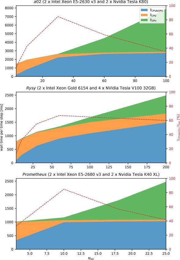
4490                                                                               P. Dziekan and P. Zmijewski: UWLCM 2.0

ulations model a volume of the order of several cubic meters,       solver (Smolarkiewicz and Margolin, 2000). Diffusion of Eu-
not enough to capture many important cloud-scale processes.         lerian fields caused by subgrid-scale (SGS) turbulence can
Whole clouds and cloud fields can be modeled with the large-        be modeled with a Smagorinsky-type model (Smagorinsky,
eddy simulation (LES) technique. In LES, small-scale eddies         1963) or with the implicit LES approach (Grinstein et al.,
are parameterized, so that only large eddies, typically of the      2007).
order of tens of meters, are resolved. Thanks to this, it is fea-      Cloud microphysics can be modeled with a single- or
sible to model a domain spanning tens of kilometers.                double-moment bulk scheme or with a Lagrangian particle-
   DNS and LES models of clouds need to resolve air flow,           based model. Depending on the microphysics model, sim-
which is referred to as cloud dynamics, and the evolution           ulations are named UWLCM-B1M (single-moment bulk
of cloud droplets, which is known as cloud microphysics.            scheme), UWLCM-B2M (double-moment bulk scheme) or
UWLCM is a tool for LES of clouds with a focus on detailed          UWLCM-SDM (super-droplet method). Details of micro-
modeling of cloud microphysics. Dynamics are represented            physics models can be found in Arabas et al. (2015). In
in an Eulerian manner. Cloud microphysics are modeled in a          both bulk schemes, cloud water and rain water mixing ra-
Lagrangian particle-based manner based on the super-droplet         tios are prognostic Eulerian variables. In the double-moment
method (SDM) (Shima et al., 2009). Lagrangian particle-             scheme, cloud droplet and rain drop concentrations are also
based cloud microphysics models have gained popularity in           prognostic Eulerian variables. In the Lagrangian particle-
the last decade (Shima et al., 2009; Andrejczuk et al., 2010;       based scheme, all hydrometeors are modeled in a Lagrangian
Riechelmann et al., 2012). These are very detailed models           manner. The scheme is based on the super-droplet method
applicable both to DNS and LES. Their level of detail and           (SDM) (Shima et al., 2009). In particular, it employs the all-
computational cost are comparable to the more traditional           or-nothing coalescence algorithm (Schwenkel et al., 2018).
Eulerian bin models, but Lagrangian methods have several            In SDM, a relatively small number of computational parti-
advantages over bin methods (Grabowski et al., 2019). Sim-          cles, called super-droplets (SDs), represent the vast popula-
pler, Eulerian bulk microphysics schemes are also available         tion of all droplets. Equations that govern the behavior of
in UWLCM.                                                           SDs are very similar to the well-known equations that gov-
   We start with a brief presentation of the model, with par-       ern the behavior of real droplets. The condensation equa-
ticular attention given to the way the model was adapted to         tion includes the Maxwell–Mason approximation and the κ-
distributed memory systems. This was done using a mixed             Köhler parameterization of water activity (Petters and Krei-
OpenMP–message passing interface (MPI) approach. Next,              denweis, 2007). SDs follow the resolved, large-scale flow
model performance is tested on single-node systems fol-             and sediment at all times with the terminal velocity. The ve-
lowed by tests on a multi-node system. The main goals of            locity of SDs associated with SGS eddies can be modeled
these tests are to determine simulation parameters that give        as an Ornstein–Uhlenbeck process (Grabowski and Abade,
optimal use of computing hardware and check model scal-             2017). Collision–coalescence of SDs is treated as a stochas-
ing efficiency. Other discussed topics are the GPU vs. CPU          tic process in which the probability of collision is propor-
speedup and performance of different MPI implementations.           tional to the collision kernel. All particles, including hu-
                                                                    midified aerosols, are modeled in the same way. There-
                                                                    fore, particle activation is resolved explicitly, which often re-
2   Model description                                               quires short time steps for solving the condensation equation.
                                                                    Short time steps are sometimes also required when solving
A full description of UWLCM can be found in Dziekan                 collision–coalescence. To permit time steps for condensation
et al. (2019). Here, we briefly present key features. Cloud         and collision–coalescence shorter than for other processes,
dynamics are modeled using an Eulerian approach. Eule-              two separate substepping algorithms, one for condensation
rian variables are the flow velocity, potential temperature         and one for collision–coalescence, are implemented.
and water vapor content. Equations governing the time evo-             Equations for the Eulerian variables, including cloud and
lution of these variables are based on the Lipps–Hemler             rain water in bulk microphysics, are solved by a CPU. La-
anelastic approximation (Lipps and Hemler, 1982), which is          grangian microphysics can be modeled either on a CPU or on
used to filter acoustic waves. These equations are solved us-       a GPU. In the latter case, information about super-droplets is
ing a finite difference method. Spatial discretization of the       stored in the device memory and GPU calculations can be
Eulerian variables is done using the staggered Arakawa-C            done in parallel with the CPU calculations of Eulerian vari-
grid (Arakawa and Lamb, 1977). Integration of equations             ables. Compared to UWLCM 1.0 described in Dziekan et al.
that govern transport of Eulerian variables is done with the        (2019), the order of operations has been changed to allow
multidimensional positive definite advection transport algo-        for GPU calculations to continue in parallel to the CPU cal-
rithm (MPDATA) (Smolarkiewicz, 2006). Forcings are ap-              culations of the Eulerian SGS model. An updated Unified
plied explicitly with the exception of buoyancy and pres-           Modeling Language (UML) sequence diagram is shown in
sure gradient, which are applied implicitly. Pressure per-          Fig. 1.
turbation is solved using the generalized conjugate residual

Geosci. Model Dev., 15, 4489–4501, 2022                                              https://doi.org/10.5194/gmd-15-4489-2022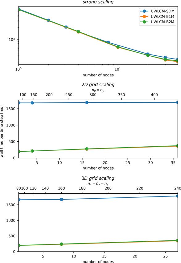
P. Dziekan and P. Zmijewski: UWLCM 2.0                                                                                  4491

Figure 1. UML sequence diagram showing the order of operations in the UWLCM 2.0 model. Right-hand-side terms are divided into
condensational, non-condensational and subgrid-scale parts; R = Rc + Rn + RSGS . Other notation follows Dziekan et al. (2019).

https://doi.org/10.5194/gmd-15-4489-2022                                           Geosci. Model Dev., 15, 4489–4501, 2022
4492                                                                              P. Dziekan and P. Zmijewski: UWLCM 2.0

  All CPU computations are done in double precision. Most
of the GPU computations are done in single precision.
The only exception is high-order polynomials, e.g., in the
equation for the terminal velocity of droplets, which are
done in double precision. So far, UWLCM has been used
to model stratocumuli (Dziekan et al., 2019, 2021b), cu-
muli (Grabowski et al., 2019; Dziekan et al., 2021b) and ris-
ing thermals (Grabowski et al., 2018).

3   Adaptation to distributed memory systems

The strategy of adapting UWLCM to distributed memory
systems was developed with a focus on UWLCM-SDM sim-
ulations with Lagrangian microphysics computed by GPUs.
Therefore, this most complicated case is discussed first. Sim-
pler cases with microphysics calculated by CPUs will be dis-
cussed afterwards.
   The difficulty in designing a distributed memory imple-
mentation of code in which CPUs and GPUs simultaneously
conduct different tasks is in obtaining a balanced workload
distribution between different processing units. This is be-      Figure 2. Visualization of the domain decomposition approach of
cause GPUs have a higher throughput than CPUs, but device         UWLCM. Top–down view on a grid with 10 cells in each horizon-
memory is rather low, which puts an upper limit on the GPU        tal direction. Scalar variables are located at cell centers and vec-
workload. Taking this into account, we chose to use a do-         tor variables are located at cell walls. Computations are divided
main decomposition approach that is visualized in Fig. 2. The     among five MPI processes, each controlling 2 GPUs and 10 CPU
                                                                  threads. Local thread/GPU rank is the rank within the respective
modeled domain is divided into equal slices along the hori-
                                                                  MPI process. Dashed lines represent boundaries over which com-
zontal x axis. Computations in each slice are done by a sin-      munications need to be done using MPI assuming periodic horizon-
gle MPI process, which can control multiple GPUs and CPU          tal boundary conditions.
threads. Cloud microphysics within the slice are calculated
on GPUs, with super-droplets residing in the device mem-
ory. Eulerian fields in the slice reside in the host memory and
their evolution is calculated by CPU threads. Since the CPU       communicators: one for the Eulerian data and one for the
and GPU data attributed to a process are colocated in the         Lagrangian data. Transfers of the Eulerian data are handled
modeled space, all CPU-to-GPU and GPU-to-CPU commu-               simultaneously by two threads, one for each boundary that is
nications happen via PCI-Express and do not require inter-        perpendicular to the x axis. This requires that the MPI imple-
node data transfer. The only inter-node communications are        mentation supports the MPI_THREAD_MULTIPLE thread
CPU-to-CPU and GPU-to-GPU. If an MPI process controls             level. Transfers of the Lagrangian data are handled by the
more than one GPU, computations within the subdomain of           thread that controls the GPU that is on the edge of the pro-
that process are divided among the GPUs also using domain         cess’ subdomain. Collective MPI communication is done
decomposition along the x axis. Intra-node communication          only on the Eulerian variables and most of it is associated
between GPUs controlled by a single process makes use of          with solving the pressure problem.
the NVIDIA GPUDirect Peer to Peer technology, which al-              It is possible to run simulations with microphysics, either
lows direct transfers between memories of different devices.      Lagrangian particle-based or bulk, computed by CPUs. In
Intra-node and inter-node transfers between GPUs controlled       the case of bulk microphysics, microphysical properties are
by different processes are handled by the MPI implementa-         represented by Eulerian fields that are divided between pro-
tion. If the MPI implementation uses the NVIDIA GPUDi-            cesses and threads in the same manner as described in the
rect Remote Direct Memory Access (RDMA) technology,               previous paragraph, i.e., like the Eulerian fields in UWLCM-
inter-node GPU-to-GPU transfers go directly from the device       SDM. In UWLCM-SDM with microphysics computed by
memory to the interconnect, without host memory buffers.          CPUs, all microphysical calculations in the subdomain be-
   Computations are divided between CPU threads of a pro-         longing to a given MPI process are divided amongst the pro-
cess using domain decomposition of the process’ subdomain         cess’ threads by the NVIDIA Thrust library (Bell and Hobe-
but along the y axis. The maximum number of GPUs that             rock, 2012).
can be used in a simulation is equal to the number of cells          File output is done in parallel by all MPI processes using
in the x direction. MPI communications are done using two         the parallel HDF5 C++ library (The HDF Group).

Geosci. Model Dev., 15, 4489–4501, 2022                                             https://doi.org/10.5194/gmd-15-4489-2022
P. Dziekan and P. Zmijewski: UWLCM 2.0                                                                                       4493

4     Performance tests                                               The total time of CPU (GPU) computations is tCPU    tot =
                                                                                        tot
                                                                  tCPU + tCPU&GPU (tGPU = tGPU + tCPU&GPU ). The degree to
4.1    Simulation setup                                           which CPU and GPU computations are parallelized is
                                                                  measured with tCPU&GPU /ttot . The timings tCPU , tGPU and
Model performance is tested in simulations of a rising moist      tCPU&GPU are obtained using a built-in timing functional-
thermal (Grabowski et al., 2018). In this setup, an initial       ity of UWLCM that is enabled at compile time by setting
spherical perturbation is introduced to a neutrally stable at-    the UWLCM_TIMING CMake variable. The timing func-
mosphere. Within the perturbation, water vapor content is in-     tionality does not have any noticeable effect on simulation
creased to obtain RH = 100 %. With time, the perturbation         wall time. The timer for GPU computations is started by a
is lifted by buoyancy and water vapor condenses within it.        CPU thread just before a task is submitted to the GPU and is
We chose this setup because it has significant differences in     stopped by a CPU thread when the GPU task returns. There-
buoyancy and cloud formation already at the start of a simu-      fore GPU timing in tCPU&GPU and in tGPU includes the time
lation. This puts the pressure solver and microphysics model      it takes to dispatch (and to return from) the GPU task.
to test without the need of a spinup period.
   Subgrid-scale diffusion of Eulerian fields is modeled with     4.4   Single-node performance
the Smagorinsky scheme. The SGS motion of hydromete-
ors is modeled with a scheme described in Grabowski and           In this section we present tests of the computational per-
Abade (2017). Model time step length is 0.5 s. Substepping        formance of UWLCM-SDM run on a single-node system.
is done to achieve a time step of 0.1 s for condensation and      The goal is to determine how the parallelization of CPU and
coalescence. These are values typically used when modeling        GPU computations can be maximized. We also estimate the
clouds with UWLCM. No output of model data is done.               speedup achieved thanks to the use of GPUs. No MPI com-
                                                                  munications are done in these tests. The size of the Eulerian
4.2    Computers used                                             computational grid is 128 × 128 × 128 cells. In the super-
                                                                  droplet method, the quality of the microphysics solution de-
Performance tests were run on three systems: “Rysy”, “a02”        pends on the number of super-droplets. We denote the initial
and “Prometheus”. Hardware and software of these systems          number of super-droplets per cell by NSD . We perform a test
are given in Tables 1 and 2, respectively. Rysy and a02 were      for different values of NSD . The maximum possible value of
used only in the single-node tests, while Prometheus was          NSD depends on available device memory.
used both in single- and multi-node tests. Prometheus has             The average wall time it takes to do one model time step
72 GPU nodes connected with Infiniband. We chose to use           is plotted in Fig. 3. The time complexity of Eulerian com-
the MVAPICH2 2.3.1 MPI implementation on Prometheus               putations depends on grid size and, ideally, does not depend
because it supports the MPI_THREAD_MULTIPLE thread                                                    tot slightly increases with
                                                                  on NSD . In reality, we see that tCPU
level, is CUDA-aware and is free to use. Another implemen-        NSD . The space and time complexity of Lagrangian compu-
tation that meets these criteria is OpenMPI, but it was found     tations increases linearly with NSD (Shima et al., 2009). It
to give greater simulation wall time in scaling tests of “libm-                  tot in fact increases linearly with N , except
                                                                  is seen that tGPU                                     SD
pdata++” (Appendix B). The NVIDIA GPUDirect RDMA                  for low values of NSD . For NSD = 3, CPU computations take
was not used by the MPI implementation because it is not          longer than GPU computations (tCPU   tot > t tot ) and almost all
                                                                                                              GPU
supported by MVAPICH2 for the type of interconnect used           GPU computations are done in parallel with CPU computa-
on Prometheus. MVAPICH2 does not allow more than one              tions (tGPU ≈ 0). As NSD is increased, we observe that both
GPU per process. Therefore multi-node tests were done for         ttot and tCPU&GPU increase, with tCPU&GPU increasing faster
two processes per node, each process controlling 1 GPU and        than ttot , and that tCPU decreases. This trend continues up to
12 CPU threads.                                                   some value of NSD , for which tCPU  tot ≈ t tot . Parallelization
                                                                                                              GPU
                                                                  of CPU and GPU computations (tCPU&GPU /ttot ) is highest
4.3    Performance metrics                                        for this value of NSD . If NSD is increased above this value,
                                                                  GPU computations take longer than CPU computations, ttot
The wall time taken to complete one model time step ttot is       increases linearly and the parallelization of CPU and GPU
divided into three parts: ttot = tCPU +tGPU +tCPU&GPU , where     computations decreases. The threshold value of NSD depends
                                                                  on the system; it is 10 on Prometheus, 32 on a02 and 64
    – tCPU is the time when the CPU is performing work and
                                                                  on Rysy. This difference comes from differences in relative
      the GPU is idle,
                                                                  CPU-to-GPU computational power between these systems.
    – tGPU is the time when the GPU is performing work and        In LES, NSD is usually between 30 and 100. The test shows
      the CPU is idle,                                            that high parallelization of CPU and GPU computations, with
                                                                  tCPU&GPU /ttot up to 80 %, can be obtained in typical cloud
    – tCPU&GPU is the time when the CPU and the GPU are           simulations.
      performing work simultaneously.

https://doi.org/10.5194/gmd-15-4489-2022                                            Geosci. Model Dev., 15, 4489–4501, 2022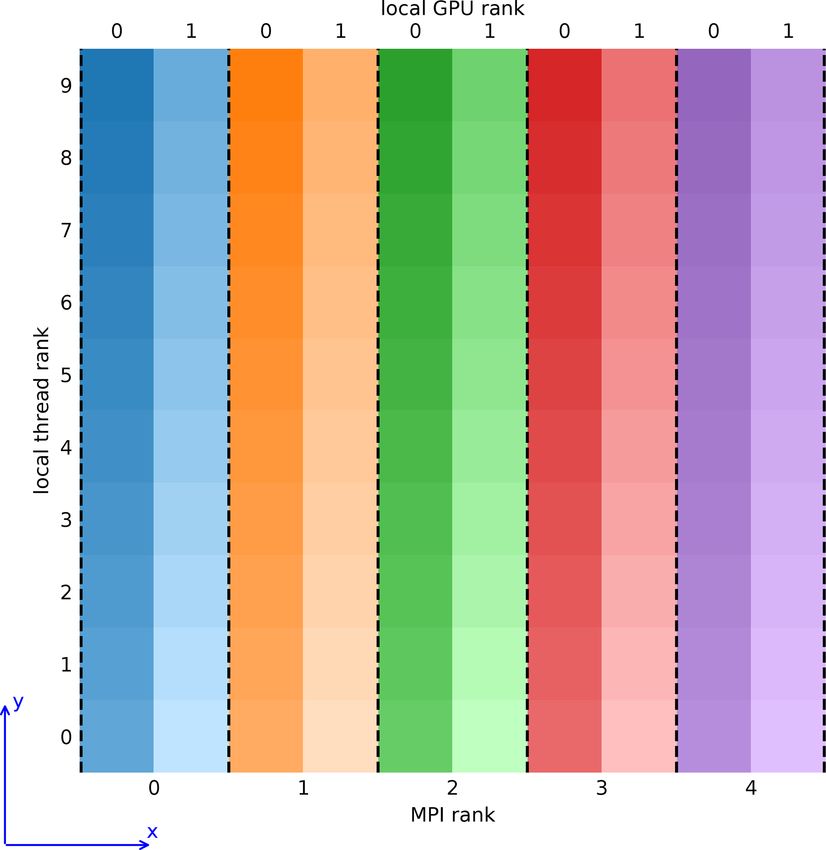
4494 P. Dziekan and P. Zmijewski: UWLCM 2.0
Table 1. List of hardware on the systems used. Computing performance and memory bandwidths are maximum values provided by the
processing unit producer. Power usage of a processing unit is measured by the thermal design power (TDP).
Rysy a02 Prometheusa
CPUs 2× Xeon Gold 6154 @ 2.50 GHz 2× Xeon E5-2630 v3 @ 2.40 GHz 2× Xeon E5-2680 v3 @ 2.50 GHz
GPUs 4× Tesla V100 2× Tesla K80 2× Tesla K40 XL
CPU cores 2 × 18 2×8 2 × 12
CPU performance 2 × 1209.6 Gflops 2 × 307.2 Gflops 2 × 480 Gflops
GPU performanceb 4 × 14.028 (7.014) Tflops 2 × 8.73 (2.91) Tflops 2 × 5.34 (1.78) Tflops
CPU TDP 2 × 200 W 2 × 85 W 2 × 120
GPU TDP 4 × 250 W 2 × 300 W 2 × 235 W
Host memory 384 GB 128 GB 128 GB
Device memory 4 × 32 GB 2 × 24 GB 2 × 12 GB
Host memory bandwidth 2 × 128 GB s−1 2 × 68 GB s−1 2 × 68 GB s−1
Device memory bandwidth 4 × 900 GB s−1 2 × 480 GB s−1 2 × 288 GB s−1
Host-device bandwidth (PCI-E) 4 × 15.754 GB s−1 2 × 15.754 GB s−1 2 × 15.754 GB s−1
Interconnect n/ac n/ac Infiniband 56 Gb s−1
a The cluster has 72 such nodes.
b Single-precision performance. Double-precision performance is given in brackets. Almost all GPU computations are done in single precision.
c Used in single-node tests only.
Table 2. List of software on the systems used.
Name CUDA gcc Boost HDF5 Thrust blitz++
Rysya 11.0 9.3.0 1.71.0 1.10.4 1.9.5-1 1.0.2
a02 10.1 4.8.5 1.60.0 1.8.12 1.9.7 0.10
Prometheus 11.2 9.3.0 1.75.0 1.10.7 1.10.0 1.0.2
a Software from a Singularity container distributed with UWLCM.
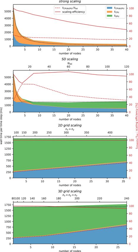
In UWLCM-SDM, microphysical computations can also ent reasons. Depending on the scenario and on the number of
be done by the CPU. From the user perspective, all that needs nodes used, the number of Eulerian grid cells is between 0.5
to be done is to specify “–backend=OpenMP” at runtime. and 18.5 million, and number of Lagrangian particles is be-
To investigate how much speedup is achieved by employing tween 40 million and 18.5 billion. Details of the simulation
GPU resources, in Fig. 4 we plot the time step wall time of setup for each scenario are given in Table 3. The scenarios
CPU-only simulations (with microphysics computed by the are
CPU) and of CPU + GPU simulations (with microphysics
computed by the GPU). The estimated energy cost per time – “strong scaling”. More nodes are used in order to de-
step is also compared in Fig. 4. We find that simulations that crease the time it takes to complete the simulation.
use both CPUs and GPUs take between 10 to 130 times less
time and use between 10 to 60 times less energy than simu- – “SD scaling”. More nodes are used to increase the to-
lations that use only CPUs. Speedup and energy savings in- tal device memory, allowing for more SD to be mod-
crease with NSD and depend on the number and type of CPUs eled, while the grid size remains the same. This results
and GPUs. It is important to note that microphysics compu- in weak scaling of the GPU workload and strong scal-
tations in UWLCM-SDM are dispatched to CPU or GPU by ing of the CPU workload. This test is applicable only to
the NVIDIA Thrust library. It is reasonable to expect that the UWLCM-SDM.
library is better optimized for GPUs because it is developed
by the producer of the GPU. – “2D grid scaling”. As more nodes are used, the num-
ber of grid cells in the horizontal directions is in-
creased, while the number of cells in the vertical is con-
4.5 Multi-node performance stant. In UWLCM-SDM, the number of SDs per cell
is constant. Therefore, as more cells are added, the to-
Computational performance of UWLCM-SDM, UWLCM- tal number of SDs in the domain increases. This re-
B1M and UWLCM-B2M on distributed memory systems is sults in weak scaling of both CPU and GPU workloads.
discussed in this section. We consider four scenarios in which This test represents two use cases: domain size increase
UWLCM is run on a distributed memory system for differ- and horizontal-resolution refinement. Typically in cloud
Geosci. Model Dev., 15, 4489–4501, 2022 https://doi.org/10.5194/gmd-15-4489-2022P. Dziekan and P. Zmijewski: UWLCM 2.0 4495
Figure 4. Wall time (a–c) and energy usage (d–f) per time step of
CPU-only simulations (blue) and simulations utilizing both CPU
and GPU (orange). In CPU-only simulations, energy usage is ttot ×
PCPU , where PCPU is the sum of thermal design power of all CPUs.
tot ×P
In CPU + GPU simulations, energy usage is tCPU tot
CPU +tGPU ×
PGPU , where PGPU is the sum of the thermal design power of all
GPUs. PCPU and PGPU are listed in Table 1. Results are aver-
aged over 100 time steps of UWLCM-SDM simulations on different
single-node machines.
UWLCM-SDM simulation time versus the number of
nodes used is plotted in Fig. 5. First, we discuss the strong
Figure 3. Single-node (no MPI) UWLCM-SDM performance for scaling scenario. We find that most of the time is spent on
different hardware. The wall time per model time step averaged CPU-only computations. This is because in this scenario
over 100 time steps. The results of LES of a rising thermal done NSD = 3, below the threshold value of NSD = 10 determined
on three different systems for a varying number of super-droplets, by the single-node test (Sect. 4.4). As more nodes are added,
NSD . tCPU , tGPU and tCPU&GPU are wall times of CPU-only, GPU- tCPU&GPU and ttot decrease. The ratio of these two values,
only and parallel CPU and GPU computations, respectively. These which describes the amount of parallelization of CPU and
timings are presented as stacked areas of different color. Total wall
GPU computations, is low (30 %) in a single-node run and
time per time step ttot is the upper boundary of the green area. The
dashed red line is the percentage of time spent on parallel CPU and
further decreases, however slowly, as more nodes are used.
GPU computations. Better parallelization of CPU and GPU computations is
seen in the SD scaling scenario. In this scenario, the CPU
workload scales the same as in the strong scaling scenario,
modeling, domain size is increased only in the horizon- but the workload per GPU remains constant. The largest
tal because clouds form only up to a certain altitude. value of tCPU&GPU /ttot , approximately 80 %, is found for
NSD = 10. The same value of NSD was found to give the
– “3D grid scaling”. Similar to 2D grid scaling, but more
highest tCPU&GPU /ttot in the single-node tests (Sect. 4.4). We
cells are used in each dimension. This would typically tot is approximately constant. Given the weak
observe that tGPU
be used to increase the resolution of a simulation.
scaling of the GPU workload in this scenario, we conclude
In each case, the maximum number of super-droplets that that the cost of GPU-GPU MPI communications is small.
fits the device memory is used in UWLCM-SDM. The only The small cost of GPU-GPU MPI communications, together
exception is the strong scaling test in which, as more nodes with the fact that for NSD > 10 the total time of computations
are added, the number of SD per GPU decreases. Note how is dominated by GPU computations, gives very high scaling
SD scaling is similar to strong scaling, but with more SDs efficiencies of around 100 %.
added as more GPUs are added. Also note that the 2D grid Among the scenarios, 2D and 3D grid scaling are weak
scaling and 3D grid scaling tests are similar, but with differ- scaling tests which differ in the way the size of CPU MPI
ences in the sizes of distributed memory data transfers. communications scales. We find that wall time per time step
https://doi.org/10.5194/gmd-15-4489-2022 Geosci. Model Dev., 15, 4489–4501, 20224496 P. Dziekan and P. Zmijewski: UWLCM 2.0 Figure 5. As in Fig. 3 but for multi-node tests done on the Prometheus cluster for different scaling scenarios. The dotted black line is perfect scaling of ttot . The solid red line is scaling efficiency, defined as ttot assuming perfect scaling divided by the actual ttot . Perfect scaling is defined in Table 3. Geosci. Model Dev., 15, 4489–4501, 2022 https://doi.org/10.5194/gmd-15-4489-2022
P. Dziekan and P. Zmijewski: UWLCM 2.0                                                                                                                                  4497

Table 3. Details of multi-node scaling tests. nx , ny and nz is the total number of Eulerian grid cells in the respective direction. NSD is
the initial number of super-droplets per Eulerian grid cell. Nnodes is the number of nodes used for the simulation. Number of Eulerian grid
cells in the domain is equal to nx × ny × nz . Number of super-droplets in the domain is equal to nx × ny × nz × NSD . Workload per CPU
is estimated assuming that it is proportional to the number of grid cells per CPU only. Workload per GPU is estimated assuming that it
is proportional to the number of super-droplets per GPU only. MPI transfers, data transfers between host and device memories, and GPU
handling of information about Eulerian cells are not included in these workload estimates. Data transfer sizes are for copies between different
MPI processes but do not include copies between host and device memories of the same process. Data transfer sizes are estimated assuming
                                                                                                                    2
that time step length and air flow velocities do not change with grid size. t 1 is the wall time on a single node. tGPU is the wall time of GPU
and CPU + GPU calculations in a simulation on two nodes.

                                                           Strong scaling          SD scaling                          2D grid scaling          3D grid scaling
                                                                                                                       √                        √3
             nx                                            240                     240                                 √Nnodes × 72             √  Nnodes × 80
                                                                                                                                                 3
             ny                                            240                     240                                    Nnodes × 72           √  Nnodes × 80
                                                                                                                                                 3
             nz                                            240                     240                                 100                         Nnodes × 80
             NSD                                           3                       Nnodes × 3                          100                      100
             Eulerian cells in domain [103 ]               13824                   13824                               Nnodes × 518.4           Nnodes × 512
             Super-droplets in domain [106 ]               41.472                  Nnodes × 41.472                     Nnodes × 51.84           Nnodes × 51.2
             Workload per CPU                              ∝ 1/Nnodes              ∝ 1/Nnodes                          const.                   const.
             Workload per GPU                              ∝ 1/Nnodes              const.                              const.                   const.
                                                                                                                          √                         2/3
             Data transfer size per CPU                    const.                  const.                              ∝ Nnodes                 ∝ Nnodes
             Data transfer size per GPU                    const.                  ∝ Nnodes                            ∝ Nnodes a               ∝ Nnodes a
             Time assuming perfect scaling                 t 1 /Nnodes                                2 )b
                                                                                   max(t 1 /Nnodes , tGPU              t1                       t1
           a Assuming that grid scaling is used to refine the resolution, as done in this paper. If it is done to increase the domain, the data transfer size per GPU
           scales in the same way as the one per CPU.
           b GPU time from two-node simulation is taken as reference because it is ca. 15 % lower than on a single node. A plausible explanation for this is that,
           although the number of SDs per GPU does not depend on the number of nodes, GPUs also store information about conditions in grid cells, and the
           number of grid cells per GPU decreases as more nodes are used. For more than two nodes, GPU calculation time is approximately the same as for two
           nodes.

ttot scales very well (scaling efficiency exceeds 95 %) and                                 scheme, is higher by a factor that depends on the number
                             tot (t tot > t tot ). The latter ob-
that ttot is dominated by tGPU                                                              of SD. In 2D grid scaling and 3D grid scaling tests of
                                    GPU     CPU
servation is consistent with the fact that the number of super-                             UWLCM-SDM there are 100 SDs per cell, which is a typical
droplets (NSD = 100) is larger than the threshold, NSD = 10,                                value used in LES. Then, on a single node, UWLCM-
determined in single-node tests. As in SD scaling, approx-                                  SDM simulations take approximately 8 times longer than
                    tot indicates the low cost of MPI com-
imately constant tGPU                                                                       UWLCM-B1M or UWLCM-B2M simulations. However,
munications between GPUs. Contrary to tGPU     tot , t tot clearly                          UWLCM-SDM scales better than UWLCM-B1M and
                                                      CPU
increases with the number of nodes. This shows that the cost                                UWLCM-B2M because scaling cost is associated with the
of CPU–CPU MPI communications is non-negligible. The                                        Eulerian part of the model and in UWLCM-SDM this cost
               tot does not cause an increase in t
increase in tCPU                                        tot because                         does not affect total wall time, as total wall time is dominated
additional CPU computations are done simultaneously with                                    by Lagrangian computations. As a result, the difference in
GPU computations and tGPU  tot > t tot in the studied range of                              wall time between UWLCM-SDM and UWLCM-B1M or
                                    CPU
the number of nodes. It is reasonable to expect that tGPU       tot                         UWLCM-B2M decreases with the number of nodes. For the
                     tot also for more nodes than used in this
scales better than tCPU                                                                     largest number of nodes used in 2D grid scaling and 3D grid
study. In that case, there should be some optimal number                                    scaling, UWLCM-SDM simulations take approximately
of nodes for which tGPUtot ≈ t tot . For this optimal number of                             5 times longer than UWLCM-B1M or UWLCM-B2M
                               CPU
nodes both scaling efficiency and parallelization of CPU and                                simulations. The strong scaling UWLCM-SDM test uses
GPU computations are expected to be high.                                                   three SDs per cell. For such a low number of SDs, time
    Comparison of scaling of ttot in UWLCM-B1M,                                             complexity of Lagrangian computations in UWLCM-SDM
UWLCM-B2M and UWLCM-SDM is shown in Fig. 6.                                                 is low and we see that the wall time and its scaling are very
UWLCM-B1M and UWLCM-B2M use simple micro-                                                   similar to that of UWLCM-B1M and UWLCM-B2M.
physics schemes that are computed by the CPU. UWLCM-
B2M, which has four Eulerian prognostic variables for
microphysics, is more complex than UWLCM-B1M, which                                         5     Summary
has two. Regardless of this, wall time is very similar for
UWLCM-B1M and UWLCM-B2M. Wall time of UWLCM-                                                A numerical model with Lagrangian particles embedded in
SDM, which uses a much more complex microphysics                                            an Eulerian fluid flow has been adapted to clusters equipped

https://doi.org/10.5194/gmd-15-4489-2022                                                                              Geosci. Model Dev., 15, 4489–4501, 2022
4498 P. Dziekan and P. Zmijewski: UWLCM 2.0
tions that use both CPUs and GPUs. We conclude that GPU
accelerators enable the running of useful scientific simulation
on single-node systems at a decreased energy cost.
Computational performance of the model on a distributed
memory system was tested on the Prometheus cluster. We
found that the cost of communication between nodes slows
down computations related to the Eulerian part of the model
by a much higher factor than computations related to the
Lagrangian part of the model. For example, in a weak scal-
tot is approximately 3 times
ing scenario (3D grid scaling) tCPU
larger on 27 nodes than on one node, while tGPU tot is in-
creased by only around 7 % (Fig. 5). The reason why Eu-
lerian computations scale worse than Lagrangian computa-
tion is that solving the pressure perturbation, which is done
by the Eulerian component, requires collective communi-
cations, while the Lagrangian component requires peer-to-
peer communications only. In single-node simulations on
Prometheus an optimal ratio of CPU to GPU workloads is
seen for 10 Lagrangian particles per Eulerian cell. In the lit-
erature, the number of Lagrangian particles per Eulerian cell
is typically higher: between 30 and 100 (Shima et al., 2009;
Dziekan et al., 2019, 2021b). When such a higher number
of Lagrangian particles is used in single-node simulations on
Prometheus, most of the time is spent on Lagrangian compu-
tations. However, in multi-node runs, Eulerian computation
time scales worse than Lagrangian computation time. Since
Eulerian and Lagrangian computations are done simultane-
ously, there is an optimal number of nodes for which the
amount of time during which CPUs and GPUs work in par-
allel is maximized and the scaling efficiency is high. In sce-
Figure 6. Multi-node model performance for different microphysics narios in which GPU computations take most of the time,
schemes. Wall time per model time step averaged over 100 time scaling efficiency exceeds 95 % for up to 40 nodes. The frac-
steps. Results of LES of a rising thermal done on the Prometheus tion of time during which CPUs and GPUs work in parallel
cluster for different scaling scenarios. is between 20 % and 50 % for the largest number of nodes
used. In weak scaling scenarios, the fraction of time during
which both processing units work could be increased by us-
with GPU accelerators. On multi-node systems, computa- ing more nodes, but it was not possible due to the limited
tions are distributed among processes using static domain de- size of the cluster. Single-node simulations with Lagrangian
composition. The Eulerian and Lagrangian computations are microphysics computed by GPUs are around 8 times slower
done in parallel on CPUs and GPUs, respectively. We identi- than simulations with bulk microphysics computed by CPUs.
fied simulation parameters for which the amount of time dur- However, the difference decreases with the number of nodes.
ing which CPUs and GPUs work in parallel is maximized. For 36 nodes, simulations with Lagrangian microphysics are
Single-node performance tests were done on three differ- 5 times slower, and the difference should be further reduced
ent systems, each equipped with multiple GPUs. The per- if more nodes were used.
centage of time during which CPUs and GPUs compute si- Our approach of using CPUs for Eulerian calculations and
multaneously depends on the ratio of CPU to GPU work- GPUs for Lagrangian calculations results in CPUs and GPUs
loads. GPU workload depends on the number of Lagrangian computing simultaneously for a majority of the time step
computational particles. For an optimal workload ratio, par- and gives good scaling on multi-node systems with several
allel CPU and GPU computations can take more than 80 % dozens of nodes. The same approach can be used in other
of wall time. This optimal workload ratio depends on the rel- numerical models with Lagrangian particles embedded in an
ative computational power of CPUs and GPUs. On all sys- Eulerian flow.
tems tested, the workload ratio was optimal for between 10
and 64 Lagrangian particles per Eulerian cell. If only CPUs
are used for computations, simulations take up to 120 times
longer and consume up to 60 times more energy than simula-
Geosci. Model Dev., 15, 4489–4501, 2022 https://doi.org/10.5194/gmd-15-4489-2022P. Dziekan and P. Zmijewski: UWLCM 2.0 4499
Appendix A: Software
UWLCM is written in C++14. It makes extensive use
of two C++ libraries that are also developed at the Fac-
ulty of Physics of the University of Warsaw: libmp-
data++ (Jaruga et al., 2015; Waruszewski et al., 2018) and
libcloudph++ (Arabas et al., 2015; Jaruga and Pawlowska,
2018). Libmpdata++ is a collection of solvers for general-
ized transport equations that use the multidimensional posi-
tive definite advection transport algorithm (MPDATA) algo-
rithm. Libcloudph++ is a collection of cloud microphysics
schemes.
In libcloudph++, the particle-based microphysics algo-
rithm is implemented using the NVIDIA Thrust library.
Thanks to that, the code can be run on GPUs as well as
on CPUs. It is possible to use multiple GPUs on a single
machine, without MPI. Then, each GPU is controlled by
a separate thread and communications between GPUs are
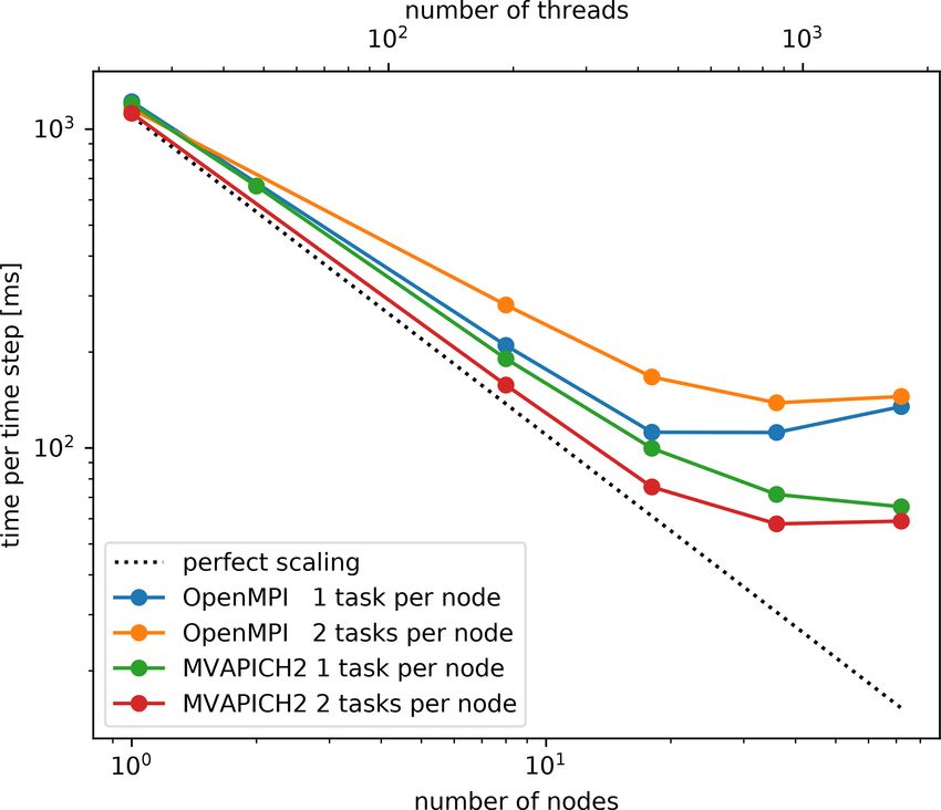
done with the asynchronous “cudaMemcpy”. Libmpdata++ Figure A1. Strong scaling test of the libmpdata++ library. Wall time
per time step of a dry planetary boundary layer simulation. The dot-
uses multidimensional array containers from the blitz++ li-
ted black line shows perfect scaling.
brary (Veldhuizen, 1995). Threading can be done either with
OpenMP, Boost.Thread or std::thread. In UWLCM we use
the OpenMP threading as it was found to be the most ef-
ficient. Output in UWLCM is done using the HDF5 out- Appendix B: Scalability of libmpdata++
put interface that is part of libmpdata++. It is based on
UWLCM uses the libmpdata++ library for solving the equa-
the thread-safe version of the C++ HDF5 library. UWLCM,
tions that govern the time evolution of Eulerian variables.
libcloudph++ and libmpdata++ make use of various com-
The library had to be adapted for work on distributed mem-
ponents of the Boost C++ library (Boost C++ Libraries,
2022). In order to have parallel CPU and GPU computa- ory systems. The domain decomposition strategy is as in
tions in UWLCM, functions from libmpdata++ and from Fig. 2 but without GPUs. Here, we present strong scaling
libcloudph++ are launched using std::async. UWLCM, lib- tests of standalone libmpdata++. The tests are done using a
dry planetary boundary layer setup, which is a part of the
cloudph++ and libmpdata++ are open-source software dis-
libmpdata++ test suite. The grid size is 432 × 432 × 51. Tests
tributed via the Github repository https://github.com/igfuw/
(last access: 14 April 2022). They have test suits that are au- were done on the Prometheus cluster. Note that all libmp-
tomatically run on Github Actions. To facilitate deployment, data++ calculations are done on CPUs. Two implementations
a Singularity container with all necessary dependencies is in- of MPI are tested: OpenMPI v4.1.0 and MVAPICH2 v2.3.1.
Note that Prometheus has two GPUs per node, but MVA-
cluded in UWLCM (https://cloud.sylabs.io/library/pdziekan/
PICH2 does not support more than one GPU per process, so
default/uwlcm) (last access: 14 April 2022).
two processes per node would need to be run in UWLCM-
Libcloudph++ and libmpdata++ have been adapted to
work on distributed memory systems. This has been imple- SDM. OpenMPI does not have this limitation. For this reason
mented using the C interface of MPI in libcloudph++ and the in the libmpdata++ scalability tests we consider two scenar-
Boost.MPI library in libmpdata++. Tests of the scalability of ios: one with two processes per node and the other with one
process per node. In the case with two processes per node,
libmpdata++ are presented in Appendix B.
each process controls half of the available threads. Test re-
sults are shown in Fig. A1. In general, better performance
is seen with MVAPICH2 than with OpenMPI. Running two
processes per node improves performance in MVAPICH2 but
decreases performance in OpenMPI. In the best case, scaling
efficiency exceeds 80 % for up to 500 threads.
Code and data availability. An up-to-date source code of
UWLCM, libmpdata++ and libcloudph++ is available
at https://github.com/igfuw (Cloud Modelling Group at IG-
FUW, 2022). In the study, the following code versions were used:
UWLCM v2.0 (Dziekan and Waruszewski, 2021), libmpdata++
https://doi.org/10.5194/gmd-15-4489-2022 Geosci. Model Dev., 15, 4489–4501, 20224500 P. Dziekan and P. Zmijewski: UWLCM 2.0
v2.0-beta (Arabas et al., 2021) and libcloudph++ v3.0 (Dziekan Nat. Comput. Sci., 1, 104–113, https://doi.org/10.1038/s43588-
et al., 2021a). Dataset, run scripts and plotting scripts are available 021-00023-0, 2021.
in Dziekan and Zmijewski (2021). Bell, N. and Hoberock, J.: Thrust: A Productivity-Oriented Library
for CUDA, in: GPU Computing Gems Jade Edition, Applica-
tions of GPU Computing Series, edited by Hwu, W.-m. W., Mor-
Author contributions. PD developed the model, planned the de- gan Kaufmann, Boston, 359–371, https://doi.org/10.1016/B978-
scribed work, conducted simulations and wrote the paper. PZ took 0-12-385963-1.00026-5, 2012.
part in conducting simulations and in writing the paper. Boost C++ Libraries: https://boost.org, last access: 25 May 2022.
Cloud Modelling Group at IGFUW: IGFUW code repository,
GitHub [code], https://github.com/igfuw/, last access: 25 May
Competing interests. The contact author has declared that neither 2022.
they nor their co-author has any competing interests. Dziekan, P. and Waruszewski, M.: University of Warsaw La-
grangian Cloud Model v2.0 source code, Zenodo [code],
https://doi.org/10.5281/zenodo.6390762, 2021.
Dziekan, P. and Zmijewski, P.: Data and scripts accom-
Disclaimer. Publisher’s note: Copernicus Publications remains
panying the paper “University of Warsaw Lagrangian
neutral with regard to jurisdictional claims in published maps and
Cloud Model (UWLCM) 2.0”, Zenodo [data set],
institutional affiliations.
https://doi.org/10.5281/ZENODO.5744404, 2021.
Dziekan, P., Waruszewski, M., and Pawlowska, H.: University of
Warsaw Lagrangian Cloud Model (UWLCM) 1.0: a modern
Acknowledgements. Initial work on the implementation of MPI large-eddy simulation tool for warm cloud modeling with La-
in libmpdata++ was done by Sylwester Arabas. We thank Syl- grangian microphysics, Geosci. Model Dev., 12, 2587–2606,
wester Arabas for consulting on the contents of the paper. This re- https://doi.org/10.5194/gmd-12-2587-2019, 2019.
search was supported by the PLGrid Infrastructure, by the Cyfronet Dziekan, P., Arabas, S., Jaruga, A., Waruszewski, M., Jarecka, D.,
AGH Academic Computer Centre, by the Interdisciplinary Centre Piotr, and Badger, C.: libcloudph++ v3.0 source code, Zenodo
for Mathematical and Computational Modelling of the University [code], https://doi.org/10.5281/ZENODO.5710819, 2021a.
of Warsaw, and by the HPC systems of the National Center for At- Dziekan, P., Jensen, J. B., Grabowski, W. W., and Pawlowska,
mospheric Research, Boulder, CO, USA. H.: Impact of Giant Sea Salt Aerosol Particles on Pre-
cipitation in Marine Cumuli and Stratocumuli: Lagrangian
Cloud Model Simulations, J. Atmos. Sci., 78, 4127–4142,
Financial support. This research has been supported by the Polish https://doi.org/10.1175/JAS-D-21-0041.1, 2021b.
National Science Center (grant no. 2018/31/D/ST10/01577). Grabowski, W. W. and Abade, G. C.: Broadening of cloud
droplet spectra through eddy hopping: Turbulent adia-
batic parcel simulations, J. Atmos. Sci., 74, 1485–1493,
Review statement. This paper was edited by David Ham and re- https://doi.org/10.1175/JAS-D-17-0043.1, 2017.
viewed by Jack Betteridge and one anonymous referee. Grabowski, W. W., Dziekan, P., and Pawlowska, H.: Lagrangian
condensation microphysics with Twomey CCN activation,
Geosci. Model Dev., 11, 103–120, https://doi.org/10.5194/gmd-
11-103-2018, 2018.
References Grabowski, W. W., Morrison, H., Shima, S. I., Abade, G. C.,
Dziekan, P., and Pawlowska, H.: Modeling of cloud micro-
Andrejczuk, M., Grabowski, W. W., Reisner, J., and Gadian, A.: physics: Can we do better?, B. Am. Meteorol. Soc., 100, 655–
Cloud-aerosol interactions for boundary layer stratocumulus in 672, https://doi.org/10.1175/BAMS-D-18-0005.1, 2019.
the Lagrangian Cloud Model, J. Geophys. Res.-Atmos., 115, Grinstein, F. F., Margolin, L. G., and Rider, W. J. (Eds.): Im-
D22, https://doi.org/10.1029/2010JD014248, 2010. plicit large eddy simulation: Computing turbulent fluid dynam-
Arabas, S., Jaruga, A., Pawlowska, H., and Grabowski, W. W.: lib- ics, 1st edn., vol. 9780521869, Cambridge University Press,
cloudph++ 1.0: a single-moment bulk, double-moment bulk, and ISBN: 9780511618604, 2007.
particle-based warm-rain microphysics library in C++, Geosci. Hockney, R. W. and Eastwood, J. W.: Computer
Model Dev., 8, 1677–1707, https://doi.org/10.5194/gmd-8-1677- Simulation Using Particles, 1st edn., CRC press,
2015, 2015. https://doi.org/10.1201/9780367806934, 1988.
Arabas, S., Waruszewski, M., Dziekan, P., Jaruga, A., Jarecka, D., Jaruga, A. and Pawlowska, H.: libcloudph++ 2.0: aqueous-
Badger, C., and Singer, C.: libmpdata++ v2.0-beta source code, phase chemistry extension of the particle-based cloud mi-
Zenodo [code], https://doi.org/10.5281/ZENODO.5713363, crophysics scheme, Geosci. Model Dev., 11, 3623–3645,
2021. https://doi.org/10.5194/gmd-11-3623-2018, 2018.
Arakawa, A. and Lamb, V. R.: Computational Design of the Basic Jaruga, A., Arabas, S., Jarecka, D., Pawlowska, H., Smo-
Dynamical Processes of the UCLA General Circulation Model, larkiewicz, P. K., and Waruszewski, M.: libmpdata++ 1.0: a
General Circulation Models of the Atmosphere, 17, 173–265, library of parallel MPDATA solvers for systems of gener-
https://doi.org/10.1016/b978-0-12-460817-7.50009-4, 1977. alised transport equations, Geosci. Model Dev., 8, 1005–1032,
Bauer, P., Dueben, P. D., Hoefler, T., Quintino, T., Schulthess, T. C., https://doi.org/10.5194/gmd-8-1005-2015, 2015.
and Wedi, N. P.: The digital revolution of Earth-system science,
Geosci. Model Dev., 15, 4489–4501, 2022 https://doi.org/10.5194/gmd-15-4489-2022P. Dziekan and P. Zmijewski: UWLCM 2.0 4501 Lipps, F. B. and Hemler, R. S.: A scale analysis of deep Smolarkiewicz, P. K.: Multidimensional positive definite advection moist convection and some related numerical calculations., transport algorithm: An overview, Int. J. Numer. Meth. Fl., 50, J. Atmos. Sci., 39, 2192–2210, https://doi.org/10.1175/1520- 1123–1144, https://doi.org/10.1002/fld.1071, 2006. 0469(1982)0392.0.CO;2, 1982. Smolarkiewicz, P. K. and Margolin, L. G.: Variational Methods for Petters, M. D. and Kreidenweis, S. M.: A single parameter Elliptic Problems in Fluid Models, in: Proc. ECMWF Work- representation of hygroscopic growth and cloud condensa- shop on Developments in numerical methods for very high reso- tion nucleus activity, Atmos. Chem. Phys., 7, 1961–1971, lution global models, Shinfield Park, Reading, 5–7 June 2000, https://doi.org/10.5194/acp-7-1961-2007, 2007. 836, 137–159, https://www.ecmwf.int/node/12349 (last access Riechelmann, T., Noh, Y., and Raasch, S.: A new method for large- 25 May 2022) 2000. eddy simulations of clouds with Lagrangian droplets includ- The HDF Group: Hierarchical Data Format, version 5, https://www. ing the effects of turbulent collision, New J. Phys., 14, 65008, hdfgroup.org/HDF5/, last access: 25 May 2022. https://doi.org/10.1088/1367-2630/14/6/065008, 2012. Veldhuizen, T.: Expression Templates, C++ report, 7, 26– Schwenkel, J., Hoffmann, F., and Raasch, S.: Improving collisional 31, https://www.cct.lsu.edu/~hkaiser/spring_2012/files/ growth in Lagrangian cloud models: development and verifica- ExpressionTemplates-ToddVeldhuizen.pdf (last access: 25 tion of a new splitting algorithm, Geosci. Model Dev., 11, 3929– May 2022), 1995. 3944, https://doi.org/10.5194/gmd-11-3929-2018, 2018. Waruszewski, M., Kühnlein, C., Pawlowska, H., and Smo- Shima, S., Kusano, K., Kawano, A., Sugiyama, T., and larkiewicz, P. K.: MPDATA: Third-order accuracy Kawahara, S.: The super-droplet method for the numeri- for variable flows, J. Comput. Phys., 359, 361–379, cal simulation of clouds and precipitation: A particle-based https://doi.org/10.1016/j.jcp.2018.01.005, 2018. and probabilistic microphysics model coupled with a non- hydrostatic model, Q. J. Roy. Meteor. Soc., 135, 1307–1320, https://doi.org/10.1002/qj.441, 2009. Smagorinsky, J.: General Circulation Experiments with the Primitive Equations, Mon. Weather Rev., 91, 99–164, https://doi.org/10.1175/1520- 0493(1963)0912.3.CO;2, 1963. https://doi.org/10.5194/gmd-15-4489-2022 Geosci. Model Dev., 15, 4489–4501, 2022
You can also read