Reflection imaging of complex geology in a crystalline environment using virtual-source seismology: case study from the Kylylahti polymetallic ...
←
→
Page content transcription
If your browser does not render page correctly, please read the page content below

Solid Earth, 13, 705–723, 2022
https://doi.org/10.5194/se-13-705-2022
© Author(s) 2022. This work is distributed under
the Creative Commons Attribution 4.0 License.

Reflection imaging of complex geology in a crystalline environment
using virtual-source seismology: case study from the Kylylahti
polymetallic mine, Finland
Michal Chamarczuk1 , Michal Malinowski1,2 , Deyan Draganov3 , Emilia Koivisto4 , Suvi Heinonen2 , and Sanna Rötsä5
1 Institute
          of Geophysics, Polish Academy of Sciences, 01-452, Warsaw, Poland
2 Geological Survey of Finland, 02151 Espoo, Finland
3 Department of Geoscience and Engineering, Delft University of Technology, Stevinweg 1, 2628 CN Delft, the Netherlands
4 Department of Geosciences and Geography, University of Helsinki, 00014 Helsinki, Finland
5 Boliden Kevitsa Mining Oy, 99670 Petkula, Finland

Correspondence: Michal Chamarczuk (chamarczukm@gmail.com)

Received: 27 November 2021 – Discussion started: 14 December 2021
Revised: 10 February 2022 – Accepted: 10 February 2022 – Published: 22 March 2022

Abstract. For the first time, we apply a full-scale 3D seis-     within the target formation and the general dipping trend of
mic virtual-source survey (VSS) for the purpose of near-mine     the formation, the selected subset is most efficient in resolv-
mineral exploration. The data were acquired directly above       ing the base of formation.
the Kylylahti underground mine in Finland. Recorded am-
bient noise (AN) data are characterized using power spec-
tral density (PSD) and beamforming. Data have the most
energy at frequencies 25–90 Hz, and arrivals with velocities     1   Introduction
higher than 4 km s−1 have a wide range of azimuths. Based
on the PSD and beamforming results, we created 10 d sub-         Ambient noise (AN) seismic interferometry (SI) principles
set of AN recordings that were dominated by multi-azimuth        can be used to extract the reflection response of the subsur-
high-velocity arrivals. We use an illumination diagnosis tech-   face at different scales (Daneshvar et al., 1995; Draganov et
nique and location procedure to show that the AN record-         al., 2009, 2013; Ruigrok et al., 2010; Ryberg, 2011; Quiros
ings associated with high apparent velocities are related to     et al., 2016). However, the original derivations of SI, as well
body-wave events. Next, we produce 994 virtual-source gath-      as the majority of surface seismic applications, have consid-
ers by applying seismic interferometry processing by cross-      ered relatively simple geological structures (sedimentary lay-
correlating AN at all receivers, resulting in full 3D VSS. We    ers). It was only recently that ANSI was for the first time
apply standard 3D time-domain reflection seismic data pro-       used for reflection imaging in much more complex crys-
cessing and imaging using both a selectively stacked subset      talline rock – also known as hardrock – environments. Cher-
and full passive data, and we validate the results against a     aghi et al. (2015) demonstrated that passive seismic record-
pre-existing detailed geological information and 3D active-      ings and SI are capable of providing 3D images of the mod-
source survey data processed in the same way as the passive      erately dipping folded volcanic rocks at the Lalor Lake min-
data. The resulting post-stack migrated sections show agree-     ing camp in Canada. The passive results were benchmarked
ment of reflections between the passive and active data and      against an active-source 3D survey. The final conjecture of
indicate that VSS provides images where the active-source        the Lalor Lake study was that future passive surveys should
data are not available due to terrain restrictions. We con-      be acquired with longer offsets, shorter receiver spacing, and
clude that while the all-noise approach provides some higher-    wider azimuth distribution to address the potential of the
quality reflections related to the inner geological contacts     method to produce convincing images of steeply dipping re-
                                                                 flections in crystalline rock environments.

Published by Copernicus Publications on behalf of the European Geosciences Union.
706                                                           M. Chamarczuk et al.: Reflection imaging of complex geology

   The most recent ANSI study near Marathon, Ontario,             identify noise panels containing body-wave energy in the 3D
in Canada (Dales et al., 2020) employed the abovemen-             recordings. In this paper, we further build on these earlier
tioned principles by combining a dense large receiver num-        results and present a full-scale 3D seismic VSS approach to
ber (large-N) array with an additional receiver line that had     extract the 3D reflection response from the Kylylahti passive
even denser receiver spacing than the rest of the grid. In        seismic data. To our knowledge, this is the first application
line with the already postulated selective stacking to enhance    of the full 3D ANSI approach to extract reflection response
body-wave reflections (Draganov et al., 2013), the authors        in a hardrock environment. However, it should be noted that
selectively stacked recordings (31 h out of the 30 d) along the   despite the pioneering nature of our VSS study in the context
more densely spaced receiver line. It was shown that higher-      of passive reflection imaging in hardrock environments, the
frequency (> 10 Hz) body-wave sources generated by trains         first state-of-the-art applications of VSS using data from
and cars (thus predominantly at the surface) could be used to     large-N arrays are related to arrays deployed in California,
image a major dipping layer interpreted as the gabbroic intru-    USA: the Long Beach array (Nakata et al., 2015) and the
sion that hosts Cu–PGE mineralizations in the area, the ex-       San Jacinto fault zone array (Ben-Zion et al., 2015).
tent of which provides crucial information for guiding min-          Our paper is organized as follows. We first describe the
eral exploration. At the same time, the authors concluded that    Kylylahti 3D dataset and the associated geological back-
even better imaging could have been obtained if the active        ground. Subsequently, we present an evaluation of the noise
mine were closer and blasting more frequent, also providing       characteristics, including power spectral density (PSD),
body-wave energy from beneath the array.                          beamforming, and spatiotemporal techniques dedicated to
   The study presented in this paper was also inspired by the     quantitative body-wave content assessment. Then, by apply-
pioneering work at Lalor Lake. We designed a new seismic          ing SI using cross-correlation, we obtain two sets of virtual-
experiment in order to test the feasibility of ANSI to pro-       source gathers (VSGs) at each receiver location of the ar-
duce a reflection seismic 3D image of a much more com-            ray, retrieved using (i) the 10 d when body-wave energy re-
plex medium when compared to the Lalor Lake mining camp           lated to underground sources is stronger than the constantly
setting. In 2016, we deployed a regular 3D passive seismic        present surface-wave noise and (ii) using all 30 d of data. Fi-
survey consisting of ca. 1000 receivers (details to follow in     nally, we apply conventional reflection processing to the sets
Sect. 3) recording 30 d over the polymetallic Kylylahti under-    of VSGs and compare them with the active-source process-
ground mine located in eastern Finland. The already existing      ing results as well as with the available detailed geological
detailed geological data and models as well as extensive pre-     data and models in order to verify that the presented 3D VSS
vious and new active-source reflection seismic data acquired      methodology works.
in parallel to the passive seismic survey made the area attrac-
tive for testing and validating the 3D virtual-source survey
(VSS) methodology.                                                2   Geological background
   The ore-bearing ophiolite-derived altered mafic–
ultramafic rocks are severely folded at Kylylahti and             The Kylylahti polymetallic (Cu–Co–Zn–Ni–Ag–Au) semi-
the main contacts are subvertical, constituting a challenge       massive to massive sulfide ore deposit is situated in the fa-
for surface seismic methods. Additionally, the rock proper-       mous Outokumpu mining district in eastern Finland (Fig. 1).
ties are causing contacts between various rock types to be        Because of the long exploration and mining history of the
less reflective compared with, e.g., the Lalor Lake scenario.     area, a host of geological and geophysical data and models –
However, based on earlier active-source reflection seismic        including extensive active-source reflection seismic data that
data, the main target contacts were expected to be reflective     were further expanded in parallel to the passive seismic sur-
and the active mine operations were providing body-wave           vey (Fig. 1) – are already available for assessing the results
energy sources at depth, which is beneficial for reflection       of the passive seismic survey. This is critical for validating
imaging in such complex medium. Initial attempts to work          the full-scale 3D seismic VSS approach. The Kylylahti mine
on the full 3D data (Chamarczuk et al., 2017, 2018) failed to     was open from 2012 to 2020 and has been operated by Boli-
provide a convincing image of the structures, and therefore       den since 2014. The Outokumpu ore belt comprises Pale-
our attention turned first to 2D ANSI applied along the           oproterozoic turbiditic deep-water sediments and ophiolitic
receiver lines (Väkevä, 2019; Chamarczuk et al., 2021).           slices of upper mantle rocks from oceanic lithosphere form-
Synthetic modeling results in 2D and 3D (Riedel et al.,           ing the Outokumpu nappe thrusted onto the Archaean base-
2018; Chamarczuk et al., 2021), as well as consistent 2D          ment and subsequently strongly deformed. Metamorphic al-
images of the main structures derived along the neighboring       teration changed the originally depleted upper mantle rocks
receiver lines, allow us to extend our work to the full 3D        into Outokumpu assemblage serpentinite–skarn–carbonate–
data with more confidence. Such an approach also allowed          quartz rocks hosting the mineralizations (Peltonen et al.,
us to test various AN preprocessing and SI techniques in a        2008). In the Kylylahti area, the following four main units
much more efficient way. Simultaneously, Chamarczuk et            can be distinguished (Peltonen et al., 2008) (Fig. 1): (1) the
al. (2019, 2020) developed a methodology to automatically         Kylylahti semi-massive to massive sulfide (S/MS) mineral-

Solid Earth, 13, 705–723, 2022                                                        https://doi.org/10.5194/se-13-705-2022
M. Chamarczuk et al.: Reflection imaging of complex geology                                                                    707

ization hosted in (2) Outokumpu ultramafics (OUMs) that            larly over the 3.5 × 3 km area with a 200 m line spacing and
mainly consist of serpentinite and talc–carbonate rocks with       50 m receiver interval (Fig. 1). Surface conditions varied be-
(3) fringed alteration zones composed of carbonate–skarn–          tween exposed bedrock and swamps.
quartz rocks, the altered Outokumpu ultramafics (OMEs).               Each receiver station consists of a Geospace GSR recorder
In combination, the nearly N–S-trending and nearly vertical        and six 10 Hz geophones, bunched together and buried when-
OUM and OME units are called the Outokumpu assemblage              ever possible, recording at a 2 ms sample rate 20 h d−1 for
rocks (referred to as the Kylylahti formation).                    30 d. As a result, we recorded over 600 h of ambient noise
   In the Kylylahti area, the Outokumpu assemblage rocks           data per receiver. In addition, the 3D grid recorded irregu-
are in nearly vertical contact with the (4) regional Kaleva        larly distributed active shots (both explosives and vibroseis)
Sedimentary Belt (KAL), consisting of mica schist and black        specifically designed for the 3D active survey (Singh et al.,
schist. Black schists often interweave with the Outokumpu          2019) as well as active shots used for the 2D seismic profiles
assemblage package, with various rock contacts repeated            crossing the 3D grid (Heinonen et al., 2019). Therefore, a
several times. Because of the complex geometry (see cross-         low-fold 3D active-source seismic survey was also acquired
section in Fig. 1), the Kylylahti formation remains a dif-         to benchmark the results of the passive survey. The active-
ficult target for surface seismic methods. Besides the ob-         source data (30 s long windows including the active shots)
vious strong impedance contrast between the S/MS miner-            were removed from the passive data before the analyses pre-
alizations and the host rocks, rock-property measurements          sented in this paper. The survey area is located in the direct
(Luhta, 2019) indicate sufficiently strong contrasts in acous-     vicinity of the town of Polvijärvi (Fig. 1). Two fairly busy
tic impedances, in the Kylylahti area mainly arising from          state roads cut through the survey area. A roundabout con-
contrasts in densities, to produce a detectable reflection at      necting both roads is located in the center of the array. The
the contact of the OUM/OME rocks and the interlayered              Kylylahti mine is located to the northwest from the round-
and surrounding schists. Some reflectivity is also expected        about. The access to the mine is along gravel roads, used ex-
to arise from the lithological changes within the Outokumpu        tensively by hauling trucks. The Kylylahti mine was active
assemblage, especially due to the alterations (e.g., the talc–     during the whole recording period. Routine mining activi-
carbonate rocks exhibit a significantly lower P-wave velocity      ties included drilling (surface and underground), transport-
than the serpentinites).                                           ing ore and waste rock (surface and underground), scaling
   Based on the rich borehole data (> 1300 boreholes) a            (underground), and mine ventilation (surface) among others.
detailed geological model was created for the 3D volume            A source of strong energy is provided by mine blasts, which
covered by the boreholes by the mine operator (Boliden)            occurred daily at depths ranging from 100 m down to approx-
and used to create a seismogeological model by Riedel et           imately 800 m below the surface.
al. (2018). The geological model was averaged into the
above-described four main units and populated with the av-
erage P-wave velocities and densities from laboratory mea-         4   Data processing and results
surements on core samples. This model was used, e.g., by
Chamarczuk et al. (2021) to assess the results of the 2D ANSI      As advocated, e.g., by Draganov et al. (2013), for reflection
based on synthetic and field data, and it is used in this paper    retrieval from ANSI, a form of selective stacking is typically
to validate the results and to support the interpretation. How-    required. Towards this end, Chamarczuk et al. (2019) devel-
ever, it should be noted that the geological model provides        oped a two-step wave-field evaluation and event detection
a reliable account of the geology only within the extent of        method (TWEED) to be able to identify noise panels contain-
the borehole data, as further discussed when describing the        ing body-wave energy. This method was later augmented by
interpretation of the passive images presented in this paper.      a machine-learning approach to automatically classify (clus-
                                                                   ter) different noise sources present in the continuous record-
                                                                   ings (Chamarczuk et al., 2020). TWEED was used to iden-
3   Data                                                           tify noise sources that were subsequently used for 2D ANSI
                                                                   imaging comparing the all-noise approach (i.e., stacking all
The passive seismic experiment was performed in the Ky-            the data) vs. the selective stacking approach using subsets of
lylahti mine area between early August and late September          the evaluated noise panels (Chamarczuk et al., 2021). At the
2016 as a part of the COGITO-MIN (COst-effective Geo-              same time, various AN preprocessing and SI techniques (e.g.,
physical Imaging Techniques for supporting Ongoing MIN-            cross-correlation vs. multidimensional deconvolution) were
eral exploration in Europe; Koivisto et al., 2018) project. This   tested at the selected receiver lines from the full array. Over-
project aimed for development of an efficient integrated ex-       all, the methodology adopted in this study builds on these
ploration workflow ranging from regional-scale exploration         earlier results and can be summarized as follows: (1) general
to detailed resource delineation and mine planning including       description of the recorded wave field to identify dominant
an active-source and passive seismic component. We used            frequencies, directions of illumination, and apparent veloci-
994 vertical-component receiver stations distributed regu-         ties of the AN sources; (2) quantification of body-wave en-

https://doi.org/10.5194/se-13-705-2022                                                          Solid Earth, 13, 705–723, 2022
708                                                                M. Chamarczuk et al.: Reflection imaging of complex geology

Figure 1. Location of the Kylylahti mine and Kylylahti array in the Outokumpu belt (top left panel). Location of the 3D passive seismic
survey (top right panel). B–B0 is a cross-section through the Kylylahti deposit (bottom left panel; modified after Peltonen et al., 2008, and
Riedel et al., 2018). Orange lines mark a representative crossline and inline location of the 3D passive seismic volume. A1–A5 denote five
representative areas of ambient noise in the Kylylahti area that are used to compute power spectral density (PSD) in Fig. 3a: the mine (A1),
a city (A2), a roundabout (A3), a road (A4), and a quiet area (A5).

Solid Earth, 13, 705–723, 2022                                                                 https://doi.org/10.5194/se-13-705-2022

M. Chamarczuk et al.: Reflection imaging of complex geology 709
ergy present in the recorded data using the TWEED approach
and obtaining spatial distribution of the noise sources; (3) ac-
tual SI data retrieval, i.e., obtaining VSGs through cross-
correlation for the two sets of data (i) for 10 d when the body-
wave events are dominating and (ii) for the full 30 d of data;
(4) standard hardrock reflection seismic processing of the ob-
tained VSGs. The above four processing steps, together with
validation and interpretation of passive results using a di-
rect comparison to an active survey as a benchmark and to
the available detailed geological data and models as a refer-
ence, add up to the five main processing blocks forming the
full-scale 3D seismic VSS methodology for the purpose of
near-mine mineral exploration developed in this study (see
flowchart in Fig. 2, where the gray-gradient-colored blocks
in the right column indicate our modifications of the state-
of-the-art AN imaging workflow proposed by Draganov et
al., 2013).
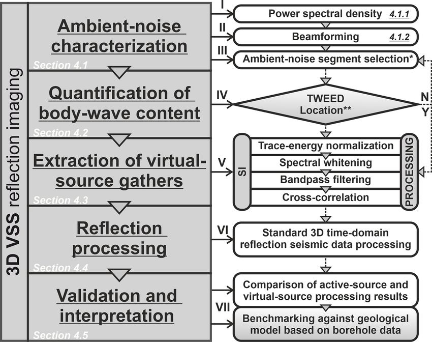
Figure 2. Summary of the 3D virtual-source survey methodology
for the purpose of near-mine mineral exploration. The left column
4.1 General ambient noise characteristics presents the core of the flowchart: it contains five main process-
ing blocks representing Sect. 4.1–4.5. The detailed processing steps
The main prerequisite for the reflection imaging based on performed within each main processing block are shown in the right
ANSI is the body-wave content in the recorded wave field column. The sequence of processing is indicated by roman numer-
(Draganov et al., 2013). We assess the body-wave con- als. Gray-gradient-colored blocks in the right column indicate our
tent in AN recordings from Kylylahti in three steps: first, modifications of the state-of-the-art ambient noise imaging work-
we determine the temporal and spatial variations of AN flow proposed by Draganov et al. (2013). The single star symbol
frequency–amplitude characteristics using power spectral denotes the user-dependent “ambient noise segment selection” pro-
density (PSD). Then, we characterize the dominant frequen- cessing step, in which the initial selection is based on the beamform-
ing results and later verified by TWEED. The double star symbol
cies and velocities of the recorded AN with beamforming,
denotes the location procedure, which supports the TWEED verifi-
and finally we directly assess the body-wave events with a
cation but is not mandatory.
dedicated detection and location procedure that provides an
objective, quantitative measure of the recorded body-wave
energy.
sources. This is clearly visible for the city area (A2) and
4.1.1 Power spectral density roundabout (A3) PSD spectra, which still contain the ener-
gies up to 90 Hz due to their proximity to the mine. The exact
We use PSD plots to assess the temporal and spatial distri- contribution from road traffic to the AN recordings from Ky-
bution of frequency–amplitude features of the seismic noise lylahti is observed in the PSD plot for stations in areas that
in the Kylylahti area. To simplify the description of AN in are located in the direct vicinity of the road (A4 and A5). The
the Kylylahti area, we analyze five representative areas (de- frequency spectra related to the road traffic exhibit the most
noted with the letter “A” in Fig. 1) that allow clearly empha- energetic parts up to 30–35 Hz, with a peak at around 20–
sizing the differences in frequency–amplitude content of the 30 Hz, which is also characteristic for the surface waves ob-
data recorded in different parts of the array. These are the served, e.g., in 2D active-source data (Heinonen et al., 2019).
mine (A1) (A2), a roundabout (A3), a road (A4), and a quiet It can be concluded that the main source of higher frequen-
area (A5). For each area, we take data from five adjacent sta- cies (25–90 Hz) in the recording area is the mine and that the
tions from the Kylylahti array, split their continuous noise higher-frequency part of AN generated in this area is still
records into 0.5 h long windows with 50 % overlap, compute recorded even in the far end of the Kylylahti array (note that
the PSD, and average the PSD values over these five stations the energies associated with the frequency range 40–90 Hz
(Fig. 3). are still visible in PSDs for receiver lines 15–19 in Fig. 3b).
The frequency spectra related to the mine (A1 in Fig. 3a) However, due to the remoteness of areas A4 and A5 (see
exhibit the broadest frequency range out of all areas, with Fig. 1), the PSD computed for receiver lines located in these
the most energetic part between 25 and 90 Hz. With increas- regions exhibits lower amplitudes in the frequency range 40–
ing distance from the mine, we observe diminishing energies 90 Hz compared to road-traffic-induced energies (10–30 Hz).
related to the higher frequencies, as well as strengthening of This is further confirmed by PSD computed for the whole ar-
the contribution from energies in the lower-frequency range ray (Fig. 3b); the transition from higher to lower frequencies
(10–30 Hz) associated with the road traffic and other surface is observed for subsequent receiver lines. Due to the differ-
https://doi.org/10.5194/se-13-705-2022 Solid Earth, 13, 705–723, 2022
710                                                                 M. Chamarczuk et al.: Reflection imaging of complex geology

Figure 3. Temporal (a) and spatial (b) variation of noise spectrograms. (a) Each panel represents power spectral densities (PSDs) computed
for each day of recording using receiver stations located in the representative areas highlighted in Fig. 1. Days highlighted with green arrows
correspond to beamforming panels highlighted with green circles in Fig. 4a. (b) PSD for a single day of recording using every receiver station
of the Kylylahti array. White dashed lines highlight receiver stations corresponding to the representative areas shown in (a). Amplitudes are
independently normalized in each panel. Two regimes of high power density are observed at frequency ranges of 10–30 and 40–90 Hz.

ence between PSD spectra associated with the road traffic                 Fig. 4b represent the dominant AN contributions that were
and mine area, we identify the higher frequencies generated               persistent during most of the recording time and which can
in the mine area as potentially associated with body-wave                 be identified in the daily beamforming plots (compare indi-
sources required for SI reflection imaging.                               vidual panels in Fig. 4a). The recorded wave field is coming
                                                                          from the NNW, a narrow area in the E, and a broad range of
4.1.2   Beamforming                                                       azimuths in the SE. These directions are consistent with the
                                                                          general orientation of areas indicated in the PSD plots and as-
After the PSD analysis, we use beamforming to assess how                  sociated with noise sources located at the mine site (A1), the
much and which parts of the data are dominated by body-                   town of Polvijärvi (A2), and the roads (A3, A4, and A5). We
wave events such that, when stacked, they would allow ob-                 can distinguish three groups of arrivals based on the apparent
taining the omnidirectional coverage of the stationary-phase              velocities (Fig. 4b): (1) V = 1–3 km s−1 likely representing
regions (Snieder, 2004). In Fig. 4a we show the results of                surface waves (associated with S, and SE areas), (2) V = 3–
standard beamforming (Rost and Thomas, 2002) analyses                     4 km s−1 likely associated with S-wave arrivals (mostly SE
calculated and summed over 20 h recorded during each sin-                 direction), and (3) V > 4.8 km s−1 interpreted as P-waves
gle day in the frequency range between 3 and 5 Hz. Note that              coming from the NNW and S directions. The red–green cir-
to avoid aliasing the theoretical limit on beamforming is im-             cle in the summed beamforming output (Fig. 4b) denotes
posed by the Nyquist wavenumber (Rost and Thomas, 2002),                  the data-driven separation between the P-waves and surface
which in the case of receiver line spacing of 200 m and ve-               waves in the Kylylahti area (note here a wide range of az-
locity of 2 km s−1 gives fmax = vmin / (21x) = 5 Hz. These                imuths associated with beamforming values above 4 km s−1
daily beamforming plots represent partial contributions to the            in Fig. 4b). The same line is projected on the results com-
stacked beamformer output in Fig. 4b, which is the summed                 puted for each day. We use this line to distinguish between
output of all 30 daily results. The maximum values shown in

Solid Earth, 13, 705–723, 2022                                                                  https://doi.org/10.5194/se-13-705-2022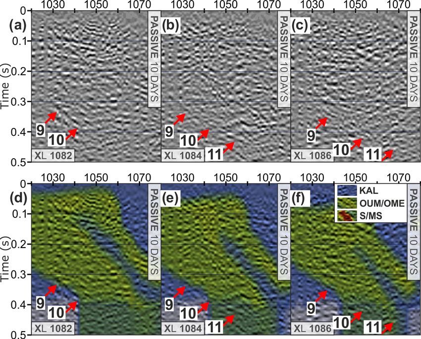
M. Chamarczuk et al.: Reflection imaging of complex geology                                                                    711

the daily beamforming results that are dominated by P-wave         model of 5 km s−1 as an approximation of the crystalline rock
arrivals (see green circles in Fig. 4a) and those with more no-    environment in the Kylylahti area. We estimate the maxi-
table surface-wave content (see red circles in Fig. 4a). It is     mum possible error from the constant-velocity model selec-
important to note here that while the number of highlighted        tion as 10 %. The computed time lags are used to time-shift
days dominated by body-wave arrivals (10) is smaller than          the cross-correlation between the every receiver pair and sum
those dominated by surface-wave sources, the body-wave ar-         the cross-correlation functions per each node of the grid. The
rivals were present during most of the recording days. As          source is found at the grid node in which the sum of the time-
shown by Draganov et al. (2013), Roots et al. (2017), and          shifted cross-correlation functions yields the highest value.
Dales et al. (2020), selecting only data periods when noise           In Fig. 5a we show an example of a noise panel contain-
is dominated by sources in the stationary-phase region for         ing a clear body-wave event detected using TWEED and
reflection retrieval may provide results with higher quality       recorded by every receiver line of the Kylylahti array. In
than stacking all noise. On the other hand, stacking all noise     Fig. 5b and c we show the InterLoc result in the horizon-
represents an attempt to utilize the full capacity of ANSI by      tal and vertical plane for the body-wave event shown in
incorporating all body-wave events which occurred during           Fig. 5a. With respect to the limited capacity of the surface
recording time but were not dominant during the days desig-        array for source depth estimation, to evaluate the approxi-
nated as dominated by surface-wave noise. To address these         mate depth of sources, we computed InterLoc results assum-
two fundamental views on SI processing, we create two sub-         ing grid points spaced at 10 m between depths of 100 and
sets of AN recordings: for 10 and 30 d, with the former rep-       800 m. In Fig. 5c, we show the exemplary results (using the
resenting selectively stacked periods of AN dominated by ar-       event from Fig. 5a) obtained for every fifth scanned depth.
rivals with high apparent velocity (these days are highlighted     The slice with the clearest focus and highest amplitude is
with green circles in Fig. 4a) interpreted to represent body-      chosen as the most probable source depth (indicated with
wave events, and the latter allows testing the full capacity of    black arrows in Fig. 5c). In Fig. 5d and e, we show the final
recorded data (see Sect. 5.5 for a more detailed discussion of     result of the joint TWEED and InterLoc approach applied to
both subsets). The subset of 10 d used for evaluation of the       the total volume of Kylylahti data showing the 3D locations
selective stacking approach in this study consists of the fol-     of all 1093 detected body-wave events (the green dot denotes
lowing days denoted in Fig. 4a: D2, D3, D7, D10, D16, D17,         the location of the exemplary event shown in Fig. 5a), which
D20, D24, D25, and D30.                                            are clustered along a conical area directly beneath the array
                                                                   (see Chamarczuk et al., 2019, for more detailed interpretation
4.2   Quantification of the body-wave content                      of the detected events). The depth range (−800 to ∼ 100 m)
                                                                   agrees with the known extent of the Kylylahti mining activi-
After the qualitative assessment of the AN sources in the Ky-      ties. The color of the dots in Fig. 5d and e represents the sep-
lylahti area, the next step is to confirm that the AN recordings   aration between body-wave events that were detected inside
associated with high apparent velocities (V > 4.8 km s−1 ),        the subset of 10 d dominated by the body-wave events (310
identified using beamforming, are related to actual body-          events marked with black dots), as indicated by the beam-
wave events. As opposed to PSD and beamforming analy-              forming (see green circles in Fig. 4a) and PSD (see green
ses, the quantification of the body-wave content is performed      arrows in Fig. 3a), and the body-wave events detected during
over short time windows (10 s long) and utilizes the afore-        the remaining 20 d (783 events marked with red dots).
mentioned TWEED method for detection of body-wave con-                Essentially, the quantification of the body-wave content
tent and InterLoc (Dales et al., 2017) for computing the loca-     shows that the passive data include a significant number of
tions of the detected sources.                                     body-wave events originating from subsurface sources. This
   The essence of TWEED (Chamarczuk et al., 2019) is that          verifies that the high-velocity arrivals observed in the beam-
it allows the detection of body-wave arrivals by scanning the      forming analysis are actually related to body-wave events
neighboring receiver lines from the regular 3D array. It en-       and not to some inline surface-wave sources. In proportion,
sures that the surface waves arriving off the line and hav-        the number of body-wave events is not any higher during the
ing apparent velocities similar to body waves are discarded.       10 d dominated by the body waves than during the rest of the
InterLoc is similar to beamforming, but instead of scanning        30 d of overall recording time. However, since these 10 d are
azimuth and velocities, it scans the different location points     characterized by noticeably lower low-velocity surface-wave
and the input comprises cross-correlated waveforms instead         activity, they are dominated by the high-velocity body waves.
of the noise panels. It is based on computation of the model-
based time lags at each scanned point of a model grid. The         4.3   Extraction of virtual-source gathers
Kylylahti formation (see description of the Outokumpu as-
semblage rocks in Sect. 2) can be considered the “inclusion”       In this subsection, we retrieve two sets of VSGs for reflection
in the simple, single-layer background (see description of the     imaging: using AN recordings from the 10 d dominated by
KAL unit in Sect. 2) and does not affect the global average        the body-wave events, during which events highlighted with
velocity. Therefore, in this study we use a constant-velocity      black dots in Fig. 5d and e occurred, and using all data (30 d).

https://doi.org/10.5194/se-13-705-2022                                                          Solid Earth, 13, 705–723, 2022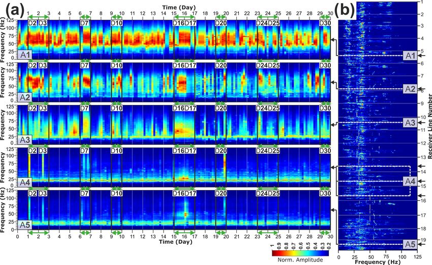
712                                                                  M. Chamarczuk et al.: Reflection imaging of complex geology

Figure 4. Directional beamforming analysis of recorded ambient noise (AN) using all available Kylylahti recordings. (a) Beamforming
outputs calculated for 20 hourly panels from 30 d of recording time. Each panel in (a) represents analysis for 1 d of recording. Panels are
displayed in chronological order. (b) Summed output of the results shown in (a). Maximum values from each hourly (a) and daily (b) result
are displayed as a function of apparent velocity and azimuth for the frequency range 3–5 Hz. The north direction (N) has an azimuth of
0◦ . The azimuth increases to the west (i.e., counterclockwise), and apparent velocities increase toward the center of the circles. Warmer
colors indicate directions of strong incoming energy. Green dashed circles in (a) highlight 10 daily AN recordings dominated by arrivals
with apparent velocities > 4.8 km s−1 and used for initial selection of the 10 d subset as the representation of the selective stacking approach
in this study. In Sect. 4.2, this initial subset of data denoted with green circles in (a) is evaluated by TWEED to confirm that the AN
recordings associated with apparent velocities > 4.8 km s−1 are related to body-wave events and eventually used to obtain the selectively
stacked virtual-source gathers shown in Figs. 6 and 7 described in Sect. 4.3. The same days are highlighted with green arrows in Fig. 3a.

The processing described in this subsection is the same for               rather than only selected 10 s time windows with the detected
both sets of data with the only difference being the number               events.
of daily recordings used as an input. As evidenced by the                    To retrieve VSGs, we divide the daily AN recordings into
daily PSD temporal variations (Fig. 3a) and the daily beam-               30 min noise panels. Prior to cross-correlation, all traces of
forming results (Fig. 4a), high-frequency and high-apparent-              each panel are normalized by applying a trace-to-trace am-
velocity arrivals occurred during most of the recording time              plitude balancing (trace energy normalization; Draganov et
(primarily associated with the mine activity). Therefore, the             al., 2013) to ensure that energy from all subsurface sources
actual number of body-wave events recorded by the Kylylahti               is equally weighted. Next, each noise panel is subjected to
array is likely higher than the number of events that were                spectral whitening such that the energy of all traces in a noise
detected with TWEED. To incorporate the possibly omitted                  panel is brought to the same level of amplitudes in the fre-
body-wave arrivals, we decided to use entire daily recordings             quency domain. The spectral whitening removes any con-

Solid Earth, 13, 705–723, 2022                                                                   https://doi.org/10.5194/se-13-705-2022

M. Chamarczuk et al.: Reflection imaging of complex geology                                                                            713

Figure 5. Performance of the combined TWEED and InterLoc processing scheme. (a) Scheduled mine event (underground blast) detected
with TWEED, representing the typical body-wave event recorded by the Kylylahti array. Horizontal black lines mark the spatial extent
of 19 receiver lines forming the complete Kylylahti array. (b) InterLoc output computed for the body-wave event shown in (a) using a
10 s recording detected with TWEED. The color scale represents the normalized amplitude of the InterLoc output. Black triangles indicate
geophone locations, and the red polygon corresponds to the mine location. (c) InterLoc output for a set of discrete depth intervals. Each
result in (c) was normalized using the global maximum from all evaluated depth intervals. The x − y section at −450 m of depth exhibiting
the clearest focus and highest amplitudes is highlighted with black arrows and represents the most probable depth of the event shown in (a).
(d) x − y and (e) 3D spatial distribution of the collection of sources at depth estimated during the 30 recording days projected on a map
with the Kylylahti array (black triangles) and geographical coordinates. Dots represent the locations of the maximum InterLoc values of each
detected body-wave event. The location of the event shown in (b) is denoted with a green circle. Black dots indicate the location of events,
which were detected inside the subset of 10 d, highlighted in Figs. 3 and 4 and used to evaluate the SI selective stacking performance. Red
dots show the locations of events from the remaining 20 d.

tributions related to noise-source wavelets and removes the             receivers, which gives 987 042 calculations per noise panel
necessity for wavelet deconvolution. The spectral whitening             and a total of 118 445 million calculations for all 1200 noise
guarantees that the amplitudes of the different frequencies in          panels). Cross-correlating a master trace with every other re-
the band of interest are equalized, while energy normaliza-             ceiver from the array using a single noise panel yields VSG
tion guarantees equalization of the amplitudes among traces             as if the shot was acquired at this master trace location. This
and among noise panels. Finally, we apply bandpass filtering            procedure is performed for each noise panel, and after pro-
(25–35–90–120 Hz) to reject parts of the spectrum associated            cessing all 1200 panels the procedure is repeated for the next
with surface waves. This simple preprocessing sequence is               master trace until all 994 receivers are used as a master trace.
known to be an effective solution in ANSI-based reflection              Consequently, we obtain 1200 VSGs for each receiver posi-
imaging studies (see, e.g., Quiros et al., 2016).                       tion. The final step is stacking VSGs from all panels per each
   For each 30 min noise panel, the cross-correlation is cal-           receiver location. Hence, we end up with the collection of
culated between specific receiver positions acting as a master          994 VSGs representing the full-scale 3D VSS as if the shots
trace (i.e., reference receiver) and every other receiver posi-         were acquired one by one at every receiver position of the
tion from the Kylylahti array (i.e., with the remaining 993             Kylylahti array.

https://doi.org/10.5194/se-13-705-2022                                                                  Solid Earth, 13, 705–723, 2022
714                                                             M. Chamarczuk et al.: Reflection imaging of complex geology

   We assess the quality of the retrieved VSGs by check-              – AGC (500 ms)
ing the feasibility of the virtual-source data to retrieve the
same reflection arrivals that are present in the active-source        – Predictive deconvolution (200/12 ms)
data. Note, though, that the complexity of the medium, as
                                                                      – Bandpass filter (20–25–100–120 Hz)
well as the relatively large receiver intervals (50 m), makes
it very difficult to follow reflections in the shot gathers even      – Mild F-X deconvolution
in the case of active data (Singh et al., 2019). Despite that,
reflections were identified in the co-located datasets. Fig-          – Top mute
ures 6 and 7 show a comparison of the selected active-source
shot gathers with the co-located VSGs. For each shot, we              – Sort to CDP
show six receiver lines to ensure that the retrieved reflec-
                                                                      – NMO correction (velocities from active data)
tions exhibit a truly 3D nature (we expect to observe the same
event on adjacent receiver lines). The VSGs were obtained by          – Post-NMO mute
cross-correlating master trace receivers 715 (Fig. 6a), 1109
(Fig. 6b), and 1556 (Fig. 7), which are located along receiver        – Stack with SQRT-fold normalization
lines 7, 11, and 15, respectively (see receivers marked with
stars in Fig. 1), with every other receiver of the Kylylahti          – Constant-velocity 2.5D Stolt migration (inlines first,
array. The arrows indicate parts of the data associated with            then crosslines)
the same reflection arrivals, as identified in the active-source
                                                                      – Mild F-X deconvolution in the crossline direction (as
gathers. Both the signal-to-noise ratio (SNR) and the move-
                                                                        interpolator of missing bins)
outs of the reflection arrivals slightly vary between passive
and active data. Furthermore, at larger offsets (off-end re-          – Whole-trace equalization
ceiver lines), the presence of artifacts in the passive data does
not allow for the recovery of reflection arrivals (see black ar-    4.5   Validation and interpretation
rows in Figs. 6 and 7 indicating the artifacts).
   Inspecting the reflection recordings from the co-located         Here, we compare the 3D active-source and virtual-source
passive and active-source data confirms that passive data al-       processing results. In both cases, we show post-stack mi-
low retrieving the reflection response of the medium, albeit in     grated data. The comparison is facilitated by the use of the
some places obscured by artifacts. Similarly to active-source       same binning grid. Empty crosslines in the passive data were
data, we expect this reflection response to be further en-          interpolated using mild F-X deconvolution. On top of the mi-
hanced by stacking and migration (Singh et al., 2019). Note         grated stacks, we also display the geological model based on
that receivers 715, 1109, and 1556 (Fig. 1) were selected such      extensive borehole data described in Sect. 2. This helps us to
that each of them is located in proximity to a different dom-       determine the location of the expected most prominent reflec-
inant noise contributor: the mine (A1), a roundabout (A3),          tivity contacts (mineralization vs. OUM/OME and the con-
and a road (A4), respectively (see Sect. 5.2 where we explain       tacts between OUM/OME and KAL). We first analyze inline
the link between AN characteristics and the VSG quality).           1040 (see Fig. 1 for location) and then several corresponding
                                                                    crosslines, for which the reflectivity between the passive and
4.4   Reflection processing                                         active data is most consistent.
                                                                       A comparison of the 3D-processed images along inline
The reflection processing workflow for the virtual-source           1040 of both surveys is shown in Fig. 8a–c and g. Red arrows
data was modified from the one derived for processing the           indicate positions of reflections associated with some main
active-source survey data (Singh et al., 2019). Despite the         lithological contacts within the ore-bearing Kylylahti forma-
fact that the active survey and VSS differ in the crossline         tion, as identified in the active data and verified by the geo-
source spacing (20–100 m vs. 200 m), we used the same size          logical model (see events marked with arrows 1–3 in Fig. 8c).
of the CDP bins (25×25 m) and the same binning grid. In the         The area marked by the blue rectangle in Fig. 8a–c and g de-
case of the passive data, this leads to some empty crosslines.      notes a gap in fold due to the active-shot distribution. In this
Considering different shot geometries and number of shots           case, the passive data supplement the image obtained from
(736 active vs. 994 virtual shots), the stacking fold is higher     the active data by providing reflectivity in places where in-
for the passive data (max. 700) compared with the active data       line 1040 from the active survey has no data (see, e.g., the
(max. 160). Below is the list of the most important process-        orange dashed line in Fig. 8b and c indicating how the con-
ing steps.                                                          tinuity of a single reflection event can be obtained by joint
  – Read VSGs                                                       analysis of active and passive data).
                                                                       In the middle row of Fig. 8, we show crossline 1068 of
  – Geometry setup (25 × 25 m bins)
                                                                    the active survey (Fig. 8d) and passive surveys obtained us-
  – Refraction statics (from active data)                           ing 10 d (Fig. 8f) and 30 d (Fig. 8e). In this case, the result

Solid Earth, 13, 705–723, 2022                                                           https://doi.org/10.5194/se-13-705-2022
M. Chamarczuk et al.: Reflection imaging of complex geology 715 Figure 6. Comparison of exemplary co-located 3D common-source gathers using active and passive data. The active-shot gathers are filtered using a bandpass filter (25–35–90–120 Hz) to have the frequency content of the passive data. For each gather, we show six receiver lines (RLs). (a) Common-source gathers co-located with receiver station 715: (top row) active-shot gather, (middle row) VSGs obtained using 30 d of noise, and (bottom row) VSGs obtained using 10 d of noise. (b) Common source gathers co-located with receiver station 1109: (top row) active-shot gather, (middle row) VSGs obtained using 30 d of noise, and (bottom row) VSGs obtained using 10 d of noise. (a) The orange and (b) blue arrows on both active and passive data highlight the position of reflection arrivals observed in active-source data and projected on co-located VSGs. Black arrows indicate artifacts characteristic for passive data. TWT stands for two-way travel time. from 10 d of AN contains mildly dipping, continuous reflec- constrained with the borehole data, and a series of repeti- tion that is associated with an internal contact between an tions of the OUM/OME units and black schist interlayers is OUM/OME unit and black schists of KAL (see event marked expected before hitting the actual base of the Kylylahti for- with arrow 6 in Fig. 8f). Note that the extent of the KAL unit mation and the surrounding mica schists. Interestingly, the surrounding the OUM/OME unit in Figs. 8 and 9 is no longer same feature is also imaged in the result from 30 d of AN https://doi.org/10.5194/se-13-705-2022 Solid Earth, 13, 705–723, 2022
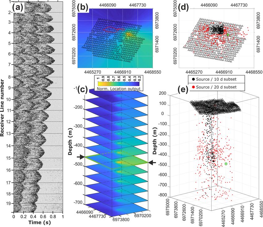
716                                                                 M. Chamarczuk et al.: Reflection imaging of complex geology

Figure 7. Comparison of exemplary co-located 3D common-source gathers using active and passive data. The active-shot gathers are filtered
using a bandpass filter (25–35–90–120 Hz) to have the frequency content of the passive data. For each gather, we show six receiver lines
(RLs). Common-source gathers co-located with receiver station 1556: (top row) active-shot gather, (middle row) VSGs obtained using 30 d
of noise, and (bottom row) VSGs obtained using 10 d of noise. The green arrows on both active and passive data highlight the position of
reflection arrivals observed in active-source data and projected on co-located VSGs. Black arrows indicate artifacts characteristic for passive
data. TWT stands for two-way travel time.

(Fig. 8e); however, it is characterized by a lower SNR and                line 1040, where the passive reflections from the right part
a different spatial extent when compared to the results from              of the bottom (arrows 1–3 in Fig. 8c) and the top (arrow 4 in
10 d (compare the event marked with arrows 7–8 in Fig. 8e                 Fig. 8c) of the OUM/OME unit shown in Figs. 8 and 9 were
with the event marked with arrow 6 in Fig. 8f). Compar-                   highlighted. On these crosslines, we consistently observe a
ing the passive results from crossline 1068 obtained from 10              weak dipping event (denoted with red arrows in Fig. 9a–
(Fig. 8f) and 30 d (Fig. 8e), we conclude that the all-noise ap-          c), which seems to correspond to the extent of the shown
proach provides higher-quality reflections related to the min-            OUM/OME unit (constrained by the extent of the borehole
eralization (see event marked with arrow 5 in Fig. 8e) and                data; see Fig. 9d–f where the geological model is overlaid on
the general dipping trend of the Kylylahti formation (note the            the same crosslines as in Fig. 9a–c). Specifically, we high-
deep reflector marked with arrows 7–8 and the overall dip of              light here crossline 1084 (Fig. 9e), where arrows 9–10 mark
the reflections in Fig. 8e), while the 10 d stack is most effi-           the continuous, dipping reflection event corresponding to the
cient in resolving the continuous reflector segment confirmed             extent of the shown OUM/OME unit, and arrow 11 is point-
by the geological model to represent a contact between the                ing to the prolongation of the same event that extends beyond
OUM/OME unit and black schists (KAL) (see arrow 6 in                      the known extent of the shown geological model based on the
Fig. 8f). This shows that the missed events in the subset of              borehole data (i.e., the bottom of the geological model).
10 d are useful and both approaches are valuable in a com-                   The Kylylahti active-source 2D and 3D data (Heinonen
plementary fashion (as shown in Draganov et al., 2013).                   et al., 2019; Singh et al., 2019) were used together with the
   For the above reasons, to showcase the consistency of                  available borehole data to interpret the base of the Kylylahti
imaging with passive survey, we focus on the clear reflection             formation (purple surface in Fig. 10). In the active-source
events associated with the contact between the OUM/OME                    data, the Kylylahti formation is characterized by piecewise
unit and black schists (KAL) at the edge of the extent of the             reflectivity, the extent of which outlines the overall forma-
borehole data used to constrain the geological model shown                tion. Because of the dominating nearly vertical orientation of
in Figs. 8 and 9 and analyze results from 10 d of AN us-                  the lithological contacts within the Kylylahti formation, the
ing three consecutive crosslines (1082, 1084, 1086; shown                 reflective segments are typically fairly short. In the active-
in Fig. 9a–c, respectively) that pass through the area of in-             source 3D data, the base of the overall Kylylahti formation,

Solid Earth, 13, 705–723, 2022                                                                  https://doi.org/10.5194/se-13-705-2022
M. Chamarczuk et al.: Reflection imaging of complex geology                                                                              717

                                                                          Figure 9. Comparison of post-stack migrated sections obtained
                                                                          from the 3D virtual-source survey along crosslines 1082 (a, d), 1084
                                                                          (b, d), and 1086 (c, f). Red arrows mark the reflection events that
                                                                          are associated with a key contact within the Kylylahti formation
                                                                          (OUM/OME in contact with black schists – KAL). Note that the
                                                                          extent of the geological model shown is constrained by the bore-
                                                                          hole data, and the marked reflections are at the very edge of this
                                                                          extent. The Kylylahti formation continues beyond the shown extent
                                                                          with further repetitions of the OUM/OME units with black schist
Figure 8. Comparison of post-stack migrated sections ob-                  interlayers. The arrows with numbers show reflections that are in-
tained from the active and passive surveys. Inline 1040 (a–c, g)          terpreted in the text. The geological model (described in Sect. 2)
and crossline 1068 (d–f, h). (a–b, d) The active-source survey.           displayed in the background is color-coded as follows: S/MS min-
(c, e, h) The 3D virtual-source survey. Red arrows mark the reflec-       eralization (red); OUM/OME units (green); KAL unit (blue).
tion events that are associated with the contacts in the geological
model and confirmed with the active-source data. The arrows with
numbers show reflections that are interpreted in the text. The ge-        5     Discussion
ological model (described in Sect. 2) displayed in the background
is color-coded as follows: S/MS mineralization (red); OUM/OME             5.1    Ambient noise characteristics
units (green); KAL unit (blue). Panels (g)–(h) show the same mi-
grated stacks as in (c) and (f), respectively, but without the geologi-
                                                                          AN characterization in this study was necessary to assess
cal model and with a broader spatial extent.
                                                                          the temporal and spatial stationarity of the noise sources and
                                                                          confirm periods of data containing body-wave illumination.
embedded in the surrounding mica schists, is also only occa-              The spatial variability of AN in the Kylylahti area is mainly
sionally associated with more continuous reflective segments              affected by the distance from the mine, and the temporal vari-
(Singh et al., 2019). In Fig. 10, we compare the interpreted              ability is mainly affected by the mine activity schedule. The
base of the Kylylahti formation to the reflection signals ob-             secondary contributions are related to the presence of roads,
served in the passive 3D cube produced from the 10 d subset               and the city of Polvijärvi. In this study, we focus on the body-
of ambient noise data dominated by the body waves. Interest-              wave retrieval, and thus we put special emphasis on parts
ingly, the base of the Kylylahti formation is on some of the              of the AN data that are characterized by AN in the higher-
crosslines and inlines (crossline 1068 and inline 1040 shown              frequency range (see parts of PSDs associated with the fre-
in Fig. 10) associated with fairly clear, more continuous re-             quency range 40–90 Hz in Fig. 3) and are mostly associated
flections that match the base of the Kylylahti formation as               with seismic events with high apparent velocities (see the ar-
interpreted from the active-source data (Fig. 10c).                       rivals with velocities > 4 km s−1 in the beamforming com-
                                                                          puted for the whole recording time in Fig. 4b). These fea-
                                                                          tures are mostly observed in the data recorded by receivers
                                                                          in the direct vicinity of the mine represented by area A1
                                                                          in Fig. 1. However, as indicated in the PSD computed for
                                                                          the whole array (Fig. 3b) and the TWEED-detected body-
                                                                          wave events induced in the vicinity of the mine (Fig. 5a), the

https://doi.org/10.5194/se-13-705-2022                                                                   Solid Earth, 13, 705–723, 2022
718 M. Chamarczuk et al.: Reflection imaging of complex geology
stations 715, 1109, and 1556, due to their proximity to areas
A1, A3, and A4 (see Fig. 1 for the location of the receivers
and the corresponding areas), respectively, are strongly af-
fected by certain AN sources: the mine (A1), a roundabout
(A3), and a road (A4). This and the possible differences in
the geophone coupling are the main reasons for differences
observed in VSGs obtained for the same amount of data. As
mentioned before, the computation of a single VSG involves
cross-correlation of a master trace with each of the remaining
993 receivers, and thus the selection of a reference receiver
has a huge impact on the quality of the VSGs. Consequently,
any bias present in the data recorded by the master traces
may influence every other trace in the VSG. To some extent,
this explains why the relatively worst performance was ob-
tained for the VSG for receiver location 1556 (Fig. 7), which
according to the PSD computed for areas A4 and A5 (see
Fig. 3a) is mostly affected by the road traffic AN. Neverthe-
less, due to the presence of higher frequencies, as well as
the confirmed recording of events induced by the mine even
at the furthest receiver lines (as evidenced in Fig. 5a), it was
still possible to retrieve reflections, albeit with lower SNR. In
addition to this, the differences between the VSGs (as well
as the difference of correlated traces within a single VSG)
obtained at different locations of the Kylylahti array were
further remedied by spectral whitening and trace energy nor-
malization (Draganov et al., 2013).
Figure 10. (a) The Kylylahti active-source 3D data processed with
We conclude that the VSGs exhibit generally lower SNR
a similar 3D reflection seismic processing workflow as the passive
compared to the co-located active-source data. On the other
3D 10 d subset data shown in (b) and overlapping the crossline
1068 and inline 1040 of the passive 3D cube in (b). The pur- hand, the migrated sections of the passive data compared
ple surface is the base of the Kylylahti formation interpreted from well to the sections from the active data (e.g., compare the
the COGITO-MIN 2D and 3D active-source data and the available active and passive image obtained for crossline 1068 shown
borehole data (c). The red surface is the Kylylahti semi-massive in Fig. 8d and e, respectively). This was possible mainly due
to massive sulfide mineralization. (d) Reflection signals associated to feasibility of SI to provide passive reflections even at the
with the base of the Kylylahti formation on the crossline 1068 and receiver lines affected by road traffic (see, e.g., receiver line
inline 1040 of the passive 3D cube highlighted with purple arrows. 15 in Fig. 7) and the higher number off all available virtual
shots (994 VSGs versus only 736 active-source gathers) used
for stacking.
aforementioned spatial and temporal variations of AN should
not preclude the retrieval of reflections from ANSI because 5.3 ANSI processing with respect to the
most of the energy associated with body waves is recorded by stationary-phase regions
the whole Kylylahti array. This is evidenced by the fact that
higher-frequency content (> 30 Hz) and body-wave events From a data processing view, two things are crucial for SI
are observed even in the southernmost receiver lines of the reflection imaging: (i) the presence of body-wave sources
Kylylahti array (receiver lines 15–19). These receiver lines and (ii) the fact that these sources must be located in
are located furthest away from the mine (see areas A4 and A5 the stationary-phase regions for reflection retrieval (Snieder,
in Fig. 1) and are mostly influenced by road traffic. In the fol- 2004; Draganov et al., 2006; Forghani and Snieder, 2010).
lowing, we discuss how these characteristics of the recorded The locations of the stationary-phase regions for reflection
noise affect the quality of the reflection content in VSGs. retrieval depend on the propagation velocity, position of the
receivers, depth of the reflector, and the angle of incidence
5.2 Impact of AN characteristics on VSG quality and reflection (Snieder, 2004; Mehta et al., 2008). Conse-
quently, calculation of the region of the stationary-phase
The receivers that were used as master traces in Figs. 6–7 sources for a retrieval of a specific reflected wave between a
were selected to showcase the VSG quality obtained in dif- virtual source and a receiver would require sufficiently accu-
ferent representative areas and based on the availability of rate knowledge of the subsurface velocity model and an indi-
co-located active-shot gathers. With this in mind, receiver vidual approach for every master–slave receiver pair. There-
Solid Earth, 13, 705–723, 2022 https://doi.org/10.5194/se-13-705-2022You can also read