Tourism informing conservation: The distribution of four dolphin species varies with calf presence and increases their vulnerability to vessel ...
←
→
Page content transcription
If your browser does not render page correctly, please read the page content below
Received: 3 September 2020        Accepted: 24 March 2021

DOI: 10.1002/2688-8319.12065

RESEARCH ARTICLE

Tourism informing conservation: The distribution of four
dolphin species varies with calf presence and increases their
vulnerability to vessel traffic in the four-island region of Maui,
Hawai‘i
Holly Self1                Stephanie H. Stack2                      Jens J. Currie2                  David Lusseau1,3

1
 School of Biological Sciences, University of
Aberdeen, Aberdeen AB24 2TZ, UK                      Abstract
2
 Pacific Whale Foundation, Wailuku, Hawaii,          1. We need reliable information about the spatial and temporal distribution of mobile
USA
                                                         species to effectively manage anthropogenic impacts to which they are exposed.
3
 National Institute of Aquatic Resources,
Technical University of Denmark, Kgs. Lyngby             Yet, we often cannot sustain dedicated annual surveys and data obtained from plat-
2800, Denmark                                            forms of opportunity offer an alternative avenue to understand where these species
                                                         spend time.
Correspondence
David Lusseau, National Institute of Aquatic         2. Four odontocete species that occur in the four-island region of Maui, Hawai’i, USA,
Resources, Technical University of Denmark,
                                                         are vulnerable to a range of human activities, but there is a lack of information
Kgs. Lyngby, 2800, Denmark.
Email: davlu@dtu.dk                                      regarding their distribution. We therefore do not know the extent of the risk these
                                                         activities present for the conservation of these species (bottlenose dolphins, spin-
Handling Editor: Mark O’Connell
                                                         ner dolphins, Pantropical spotted dolphins and false killer whales).
                                                     3. We used a cross-validated maximum entropy (MaxEnt) occupancy model to esti-
                                                         mate the distribution of these four species in an area extensively observed from
                                                         platforms of opportunity (PoP). We then determined in a similar fashion whether
                                                         the calves of those species were more likely to be observed in particular areas and
                                                         whether distribution changed with season.
                                                     4. Maxent models relying on local environmental variables described dolphin obser-
                                                         vations well (AUC > 0.7). Their distribution differed for all species when calves
                                                         were present, indicating that different environmental variables describe area use
                                                         for schools with calves present.
                                                     5. The number of sighting events of all species varied significantly with season. Bot-
                                                         tlenose dolphins and false killer whales were more prevalent in winter, while spot-
                                                         ted and spinner dolphins were more prevalent in summer.
                                                     6. We show that an overlap in the distribution of dolphin schools with calves and
                                                         vessel traffic in the region could result in collision and chronic stress risks. This
                                                         suggests a need for specific regulations for mitigating anthropogenic influences,
                                                         such as acoustic disturbance or chronic energetic disturbance from vessel traffic.

This is an open access article under the terms of the Creative Commons Attribution License, which permits use, distribution and reproduction in any medium, provided
the original work is properly cited.
© 2021 The Authors. Ecological Solutions and Evidence published by John Wiley & Sons Ltd on behalf of British Ecological Society

Ecol Solut Evid. 2021;2:e12065.                                                                                    wileyonlinelibrary.com/journal/eso3       1 of 14
https://doi.org/10.1002/2688-8319.12065
2 of 14                                                                                                                                      SELF ET AL .

                                                     This elevated risk associated with vessel traffic is likely of conservation concern
                                                     in this region for the endangered population of false killer whales and for spinner
                                                     dolphins.

                                                  KEYWORDS
                                                  cetaceans, distribution, Hawai‘i, Maxent, odontocete, Population Consequences of Disturbances,
                                                  platform of opportunity, species distribution modelling

1         INTRODUCTION                                                           While this region is considered data deficient for some species, it is
                                                                             rich in commercial and recreational vessels that can be used to collect
The extent to which anthropogenic impacts can cause conservation             opportunistic data about the location of marine wildlife (Currie et al.,
risks for highly mobile species depends on the degree of overlap in the      2018). These ‘platforms of opportunity’ (PoP) can provide an alterna-
distribution of human activities and those species (Pirotta et al., 2018).   tive way of obtaining data when costly dedicated survey effort is not
We therefore need reliable information about the species spatiotem-          feasible (Currie et al., 2018; Kiszka et al., 2007; Moura et al., 2012 ;
poral distribution to manage these risks. The conservation of popu-          Williams et al., 2018).
lations that are not exposed to direct takes, but instead face chronic           Advances in modelling approaches that can help infer species occu-
exposure to non-lethal disturbances, can be affected by reduced repro-       pancy using presence-only observations (Elith et al., 2006; Oppel et al.,
ductive success (Béchet et al., 2004; Beissinger & Peery, 2007; Crooks,      2012; Phillips, 2009), means that PoP data (Williams, Hedley, & Ham-
2002; Manlik, 2019; Manlik et al., 2016; Pirotta et al., 2018; Raithel       mond, 2018), and indeed other community science data (Currie, Stack,
et al., 2007). Habitat selection may facilitate reproductive success by      & Kaufman, 2018), can successfully be used to describe the distribution
offering better prey availability, protection from predators or reduc-       of wildlife (van Strien et al., 2013).
tion of energy expenditure by providing a more sheltered environ-                Here we used environmental variables to describe opportunistic
ment (zu Ermgassen et al., 2016). For species facing chronic exposure        observations of the four dolphin species commonly found within Maui
to anthropogenic impacts, it is important to understand not only the         four -island region. This was conducted using data obtained from tour
extent of the overlap between their range and these human activities,        operating vessels in the Maui four-island region and analysis con-
but particularly whether there is an overlap with areas where moth-          ducted using maximum entropy models to estimate their distribu-
ers and calves are more likely to be present. Areas known to have            tion in this area. Given that the identified conservation threats varied
high occurrences of juveniles or that function as nursery areas are high     between age classes (Carrillo & Ritter, 2010; Pirotta et al., 2018), we
priority for conservation efforts and protections (CBD, 2008; IUCN           assessed whether schools observed with calves differed in their distri-
Marine Mammal Protected Areas Task Force, 2018).                             bution from schools without calves. We then assessed the spatial asso-
    The Hawaiian Islands are a marine ecoregion of global importance         ciation between dolphin distribution and vessel traffic to determine
(Olson & Dinerstein, 2002). Eighteen odontocete species have been            whether there is significant overlap which could cause conservation
documented in this region, all of which are vulnerable to anthro-            concerns.
pogenic activities that have the potential to negatively impact pop-
ulation trends. These include fisheries interactions, collision and dis-
turbance risks associated with commercial or recreational vessel traf-       2       MATERIALS AND METHODS
fic (Baird et al., 2013). While many of these 18 species move through
the Maui four-island region, there is evidence that three of the dol-        2.1         Study area
phins in Hawai‘i have island-associated populations, with little docu-
mented mixing with other island populations (Carretta et al., 2020). In      The islands of Maui County; Maui, Lana’i, Moloka’i and Kaho’olawe,
the Maui four-island region, the most commonly sighted dolphins are          hereafter referred to as ‘the Maui four-island region’ lie within the
(i) the pantropical spotted dolphin, Stenella attenuata (NOAA, 2017c),       Hawaiian Islands Humpback Whale National Marine Sanctuary (HIH-
(ii) the spinner dolphin, Stenella longirostris longirostris (NOAA, 2018),   WNMS). The study area was determined by the extent of the spatial
(iii) the bottlenose dolphin, Tursiops truncatus (NOAA, 2017a), and          data available and covers an area of 1890 km2 of the contingent shelf
(iv) the false killer whale, Pseudorca crassidens (NOAA, 2013). For all      region between the four islands (Figure 1). The deepest region of the
four species, we currently lack detailed information about distribution      study area is the southern section of the ‘Alalākeiki channel, which
necessary to manage their conservation threats (Baird et al., 2013;          reaches 325 m, while the mean depth of the study area is 54 m. Anthro-
Carretta et al., 2020).                                                      pogenic activity in the region is high, with a large quantity of vessel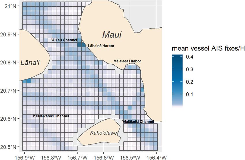
SELF ET AL .                                                                                                                                    3 of 14

F I G U R E 1 Location of the study area within the four-island region of Maui, Hawai’i, USA with mean vessel AIS fixes per hour per grid cell, data
for all vessels equipped with AIS (see Methods section) using the study area from 2013 to 2017 (BOEM & NOAA, 2019)

traffic facilitating a variety of marine tourism and recreational activi-   2.3       Data processing
ties, along with local fisheries and shipping (Figure 1) (Department of
Business Economic Development & Tourism, 2015).                             The initial dataset consisted of 2852 sightings. Which were quality con-
                                                                            trolled to ensure accurate location of sightings. Where coordinates
                                                                            were identified as erroneous (such as outside of Maui or on land), we
2.2            Cetacean observations                                        used the vessel’s built-in GPS data to correct the coordinates by iden-
                                                                            tifying the correct location of the vessel along the GPS track at the
Sightings data were collected aboard tour boats using the community         time of the sighting. For records where corrections of erroneous coor-
science application Whale and Dolphin Tracker (WDT), developed by           dinates were not possible, the sightings were excluded from analyses.
Pacific Whale Foundation (PWF) (Currie et al., 2018). While WDT is
open to the public, in this instance we restricted analyses to sightings
recorded by naturalists who have completed a 60 h training programme        2.4       Environmental data
focused on species and behaviour identification. The fleet of seven ves-
sels and each naturalist had a user account for WDT, and only this sub-     Environmental data were gridded (50 × 50 m) using the R package
set was used to ensure species identification accuracy. Only presence-      resample (Hesterberg, 2015) and associated with sightings.
only sighting locations were available, and sample bias in the form of         We introduced four spatial variables in maximum entropy (max-
numbers of sightings per grid cell was included in subsequent Max-          ent) models: bathymetry (50 m resolution) (Hawai’i Mapping Research
Ent analyses to compensate for the uneven effort associated with PoP        Group, 2017), the presence/absence of coral reefs (Andréfouët et al.,
(Pearce & Boyce, 2006).                                                     2005), the proximity to the coast (meters) for each sighting (Natural
   Dolphin sighting data were collected from multiple whale-watching        Earth, 2017) and benthic roughness. Benthic roughness was estimated
and snorkel trips departing from both Ma‘alaea and Lahaina Harbors          as the ratio of surface area to planimetric area to act as a proxy for ben-
daily between 1 January 2013 and 31 March 2017. Vessel speeds               thic habitat type (Jenness, 2004). We also used a variable that could
ranged from 5–20 knots, and followed a non-systematic track, usually        be associated with levels of anthropogenic activities: the proximity to
determined by weather and trip itinerary (e.g. snorkel site). Only sight-   urbanized coastal areas (meters) using information on urban cluster
ings where the dolphin schools were approached and subsequently             locations from census data as a proxy for coastal anthropogenic activity
watched were used in analysis to ensure accuracy of species identifi-       (State of Hawai‘i Office of Planning, 2017). We also included oceano-
cation and calf presence. Encounter location (latitude and longitude)       graphic variables: tidal height (feet) originated from the NOAA station
was recorded using WDT when the vessel was ≤150 m from the focal            1615680 at Kahului Harbour (NOAA, 2017b), sea surface tempera-
school.                                                                     ture (SST) in degrees Celsius recorded every 30 min was sourced from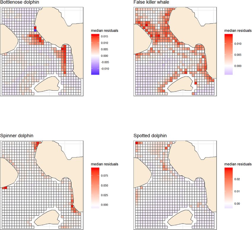
4 of 14                                                                                                                                     SELF ET AL .

FIGURE 2        Number of sightings by species per grid cell in the study region

the NOAA data buoy at station 51203 in Kaumalapau, Lana’i (NOAA,              els were trained on a k-folded subset of 70% of the data, created using
2017b) and satellite-derived ocean surface current dynamics, including        the package cvTools (Alfons, 2015). To compensate for potential effort
zonal currents velocity (m/s), zonal maximum mask (m/s), meridional           bias, an effort proxy distribution grid was established from the ker-
current velocity (m/s) and meridional current maximum mask (m/s) at a         nel density of sightings for all species; estimating the kernel utiliza-
spatial resolution of 0.33 deg (latitude) × 0.33 deg (longitude) at a 5-day   tion distribution assuming a bivariate normal kernel function using the
temporal resolution were obtained from the Jet Propulsion Laboratory          R package adehabitatHR (Calenge, 2006). We selected 10,000 spa-
‘Physical Oceanography Distributed Active Archive Data Centre’ (JPL           tial background points using this bias pattern, and further subsampled
PO.DAAC, 2017).                                                               1050 background points from those across temporal environmental
   Finally, we included temporal variables: year, to account for inter-       variables. We used those in the maxent models to assess the range of
annual variability and any influence by the El Niño–Southern Oscilla-         environmental conditions available so that the spatial distribution of
tion cycle, and season. As the oceanographic seasons in Hawai‘i are           the background points was equivalent to that of the presence records
not highly variable, we used the variance in SST (Figure 2) to define a       (Phillips, 2009; Syfert et al., 2013).
‘Winter’ season from October–April and a ‘Summer’ season from May–                 The maxent models were tested by adding and removing variables
September.                                                                    until an AUC > 0.5 was achieved indicating model performance was
                                                                              better than random, and the model with the highest AUC selected
                                                                              as the best fitting model for that species (Duque-Lazo et al, 2016 ;
2.5       Distribution model development                                      Franklin & Miller, 2010). AUC does not cover all aspects of model rele-
                                                                              vance (Lobo et al, 2008), we therefore complemented this model selec-
We categorized sightings by species and whether calves were present           tion step with estimates of model goodness-of-fit and accuracy. We
or absent in the school. We modelled each sighting response variable          evaluated the models by assessing their ability to predict the sight-
separately using ‘maxent’ in the R package dismo using a regulariza-          ings in the remaining test subset of 30% of the sighting records. We
tion factor of 1 (Hijmans et al., 2017). We preferred to carefully select     used four evaluation statistics to evaluate model fit and predictive
explanatory variables and rely on model validation rather than engage         performance: (i) the area under the receiver-operating characteristic
in a selection of penalization magnitude (Royle et al., 2012). The mod-       curve calculated with a Mann–Whitney U statistic (AUC), to indicate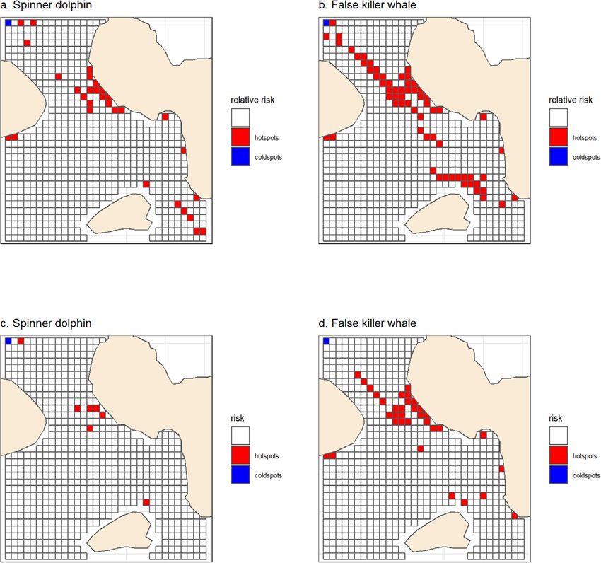
SELF ET AL .                                                                                                                                   5 of 14

discrimination performance with how much variation was captured              2.7   Assessing the influence of season on relative
by the model; (ii) the percentage correctly classified (PCC), which          abundance
described predictive performance in how many of the test sightings
were correctly predicted by the model, generated using the package           To assess seasonal variation, we modelled the number of sightings as
PresenceAbsence (Freeman & Moisen, 2015). We also used: (iii) the            a function of season (summer vs. winter) using a Generalised Linear
point biserial correlation coefficient between observed and predicted        Model with a Poisson error structure. Observations in this model were
values (COR), which described the degree to which predictions were           the number of sightings of a given species per calendar month, with a
linearly related to the established probability of presence, taking into     total of five replicates from each study year . While we did not have an
account how far predictions vary from the test values; and finally (iv)      exact measure of effort heterogeneity between seasons, the number of
the intercept of regression of observed versus predicted values (Bias),      trips during which sightings of any of the species were recorded in Win-
which indicated if the predicted values from a model are over- or            ter (1521 trips) was roughly twice the number of trips recorded in Sum-
underestimates compared to true values, generated using the custom           mer (896 trips). To ensure model assumptions had been met, graphi-
function ‘ecalp’ (Oppel et al., 2012; Phillips & Elith, 2010). Each eval-    cal plots of the residual distribution were inspected for the presence of
uation statistic provided information on a different aspect of model         patterns or bias, which was not present.
fit and performance and was examined separately for any evidence
of poor performance and cohesively to come to an overall view of
the model.                                                                   2.8       Spatial association models

                                                                             We developed spatial mixed effects models to determine the associ-
2.6            Distribution patterns                                         ation of ROR of schools with calves with the ROR of schools without
                                                                             calves and vessel traffic estimates. It is important to note that ROR
Final models for each sighting category were used to predict relative        represents central tendencies in species occurrence in each grid cells,
occurrence rate (ROR, the relative probability that a cell is contained      and therefore the association models here only capture the overlap
in a collection of presence samples) from spatial and temporal vari-         between typical vessel traffic in a grid cell and the likely presence of
ables for each species and school category (with or without calves). As      the species, discounting potential avoidance tactics the species might
it is the case for most presence-only distribution modelling efforts, we     have (e.g. Lusseau, 2005). However, these avoidance tactics can them-
do not have a way to robustly test the assumptions needed to under-          selves have conservation implications and therefore these association
stand the relationship between ROR and probability of individual pres-       models help to highlight whether vessel traffic, as a constraint on habi-
ence in a grid cell. However, the search strategy in which the vessels       tat use, may be of concern for particular species. They also discount
engage and the search intensity lead to a less effort biased sampling        uncertainties associated with the fitting of the models to the data, the
of the study area (Figure 2) than might be encountered in other com-         model validation seems to point to a lower risk associated with these
munity science project. We also accounted for a proxy of effort (Fig-        errors changing the outcome of analyses on relative trends; which is
ure S1 in the Supporting Information) in the selection of background         why we do not make any inference beyond a description of potential
points. Therefore, we assumed that ROR was an appropriate estimate           spatial concordance. Vessel density was estimated each year (2013–
of relative probability of presence (Merow et al., 2013). As we work at      2017) using the average number of automatic identification systems
a regional scale, our main focus was to understand the relative variabil-    (AIS) fixes recorded per hour in each grid cell that year using data from
ity in occurrence rather than delineate species home range. Hence, the       the U.S. Marine Cadastre (BOEM & NOAA, 2019). AIS is required for
need to define absolute probability of occurrence was not warranted          all vessel larger than 300T and all passenger vessels regardless of size.
(Merow et al., 2013; Royle et al., 2012). Finally, this means that we are    While this represents only a subset of all vessel activities, it captures
not able to compare the absolute ‘distribution’ (probability of presence)    a broad representation of vessel traffic in the area. ROR was arcsine-
between the four studied species but this does not prevent comparing         square root transformed, following investigation of the goodness-of-
general patterns of distribution (e.g. offshore vs. inshore, etc). ROR was   fit of the residual distribution with the assumed distributions, and all
estimated for each grid cell of the study area based on the median val-      models assumed a Gamma distributed error structure with a log link
ues of contributing variables for that grid cell and iteratively estimated   function. All models included a random effect of ‘year’ and ‘season’ (as
for each year and each season. ROR values for each seasonal conditions       defined in the previous section using both season and SST) as well as
were generated by supplying the 25% quantile of SST for the winter           a Matérn spatial correlation structure (Rousset & Ferdy, 2014). The
season and the 75% quantile of SST for the summer season to account          Matérn variogram function is composed of a gamma and a Bessel func-
for SST contributions over and above seasonal effects in the models.         tion and describes a generalized Gaussian spatial process with varying
Hence, cold predictions represent ROR for cold conditions (25% quan-         smoothness offering flexibility in its local behaviour.
tile SST) during winter and warm predictions represent ROR for warm             We challenged the data with five spatial models for each species
conditions (75% quantile SST) during summer. Maps of the predicted           to determine the extent with which the ROR of schools with calves
ROR were generated using ggplot2 (Wickham et al., 2018).                     (RORcalf ) was associated with the ROR of schools without calves
6 of 14 SELF ET AL .
(RORadult ) and vessel density. In all models, RORcalf was the response 3.2 Distribution model performance and
variable. A ‘null model’ only fitted an intercept as fixed effect, ‘adult validation
model’ fitted RORadult as fixed effect, an ‘AIS model’ fitted AIS as fixed
effect, an ‘adult & AIS model’ fitted a fixed effect of AIS and RORadult The models for all species were able to adequately discriminate species
and finally an ‘adult & AIS structured dispersion model’ fitted a fixed distribution patterns (AUC > 0.7) (Table 1) (Hosmer & Lemeshow,
effect of RORadult and an effect of AIS on the variance dispersion of that 1989; Phillips & Elith, 2010). The ability of the models to correctly
relationship. The latter model helped to identify whether areas where predict the test sightings varied. PCC values varied, with the lowest
RORcalf departs more from RORadult are also areas with greater vessel being for the model of false killer whale schools with calves (58%) and
density. the highest for spinner dolphin schools without calves (99%) (Table 1).
We also assessed whether RORadult was associated with vessel COR estimates of how far predictions varied from the test values fit
density by fitting two spatial mixed effects models similar to the into two broad groups: spinner dolphin schools both with and with-
ones developed for the RORcalf response variable (null model and AIS out calves, along with bottlenose dolphin schools with calves had COR
model). Models were selected using marginal AIC. All spatial mixed values above 0.3, whereas all other values were < 0.1 (Table 1). Bias
effects models were developed and fitted using spaMM in R (Rousset & showed the highest (> 6) underestimation of occurrence for false killer
Ferdy, 2014). We used this approach, rather than introduce vessel traf- whales and bottlenose dolphins, while other models had much lower
fic as an explanatory variable in the MaxEnt models as we wanted to values (< 0.6) (Table 1).
assess whether the predicted ROR might be associated with vulnera-
bility to traffic risk. Finally, if an association between vessel traffic and
distribution was detected we used a qualitative approach to determine 3.3 Variables describing distribution
a spatial index to identify vulnerability hotspots. This avoided further
manipulation of the data via regularization or scaling to get all vari- The variable contribution was varied across models (Figure 3; Table S1
ables on a similar scale in a tractable manner. For cases, where AIS in the Supporting Information). Year was the most consistent con-
was retained as an explanatory variable, we determined the ROR top tributing variable, ranked as third or higher for all models. There were
quintile cells and the AIS top quintile cells (both on a log scale given differences in the variable contribution within all species between
the distributions and assumptions of models fitted). We identified cells schools with and without calves, with spatial variables contributing
that were in both top quintiles. In cases where the structured disper- more to the distribution of schools with calves than schools without
sion model was retained, we estimated the residuals of the relationship calves.
between RORcalf and RORadult and identified the top quintile of these
residuals as a measure of relative risk. To further understand vulner-
ability in those cases, we also identified those cells were the residuals 3.4 Predicted distribution patterns
are in the top quintile, AIS is in the top quintile and RORcalf is in the top
quintile as a measure of risk. This identified locations where not only The predicted distributions revealed a variety of distribution patterns
schools with calves are more likely to be present that schools without for each species. False killer whales and bottlenose dolphins showed
calves for that species, but they are also more often present overall. We similar distributions, with high ROR for schools without calves asso-
engaged in the same process to estimate ‘coldspots’ with bottom quin- ciated with coastline and urbanized area proximity to each species,
tiles.
TA B L E 1 Statistics evaluating the predictive ability each maxent
3 RESULTS distribution model against test data
Species Calf status AUC COR Bias PCC
3.1 Sightings False killer whale Present 0.92 −0.06 0.001 0.58
Absent 0.85 −0.009 6.157 0.97
After quality control, the dataset contained 2757 sightings. The most
Bottlenose dolphin Present 0.76 0.54 0.008 0.98
frequently sighted species was spinner dolphins, totalling 1286 events.
Absent 0.94 −0.03 6.157 0.95
The highest sighting densities for spinner dolphins were recorded in
shallow coastal waters and the Au’au channel (Figure 2). Bottlenose Spotted dolphin Present 0.87 0.09 −0.01 0.80
dolphins were sighted 1106 times, distributed the most widely of the Absent 0.97 −0.01 0.003 0.96
four study species (Figure 2). Higher sighting densities of bottlenose Spinner dolphin Present 0.77 0.33 −0.02 0.63
dolphins occurred in the Au’au channel and Ma’alaea harbour. Spot- Absent 0.93 0.32 −0.03 0.99
ted dolphins were sighted most commonly in the deeper areas of the
Abbreviations: AUC, area under the receiver-operating characteristic
Au’au channel and around Lana’i, with 272 sighting recorded in total curve; Bias, intercept of regression of observed vs. predicted values; COR,
(Figure 2). Finally, 93 sightings of false killer whales were distributed point biserial correlation coefficient between observed and predicted val-
broadly across the study region (Figure 2). ues; PCC, percentage correctly classified.SELF ET AL . 7 of 14
F I G U R E 3 Variable contributions for each maxent distribution model. x: longitude, y: latitude, coast: coastal proximity, urban: urban cluster
proximity, SST: sea surface temperature, season: winter and summer season, zonevelocity: zonal currents velocity, zonemaxmask: zonal maximum
mask, medvelocity: meridonal current velocity, medmaxmask: meridional current maximum mask. (See Methods for detailed description of each
variable)
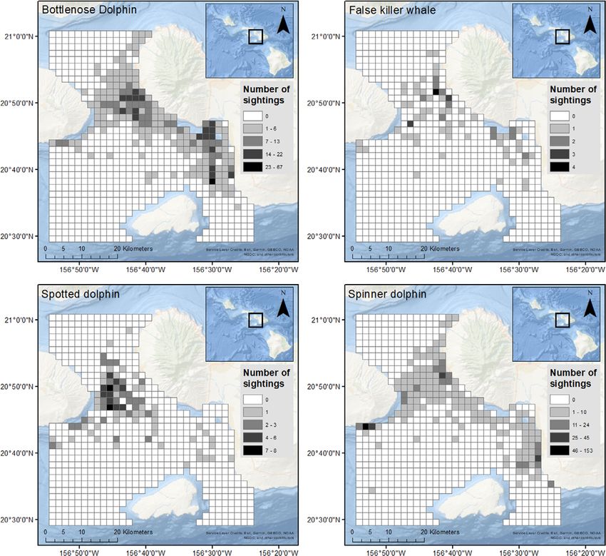
respectively. All models exhibited differences within a species depend- did not follow the same distribution as schools without calves in the
ing on whether the schools had calves, except for spotted dolphins (Fig- study area (Figure 4 and Tables 2 and 3; Figures S1–S9). The best
ures 4; Figures S1–S9 in the Supporting Information). models also included an effect of AIS on the dispersion of RORcalf for
spinner dolphins and false killer whales. Therefore, the departure of
RORcalf from predictions based on the ‘adult model’ is associated with
3.5 Spatial associations of the distribution of vessel density. We plotted the median residuals of the ‘adult model’
schools with calves (median across year and season for each grid cell) for each species (Fig-
ure 5), and this departure is mainly associated with schools with calves
For all species, best models retained a fixed effect of RORadult associ- being present more than expected in areas with high vessel density
ated with RORcalf . However, this effect is negative: schools with calves (Figure 6).8 of 14 SELF ET AL .
TA B L E 2 Model selection of spatial association mixed effects model for each species and for each school category (calf: School with calves,
no-calf: Schools without calves). Values are marginal AIC (best model in bold), NA when models were not fitted (see text for details). Model
selected are in bold
Adult and AIS
School Null model Adult and AIS structured
Species category (intercept only) AIS model Adult model model dispersion
Bottlenose dolphin RORcalf −80,971.0 −80,969.1 −81,684.5 −81,682.7 −77,830.6
RORadult −28,795.0 −28,796.0 NA NA NA
False killer whale RORcalf −37,887.1 −37,885.8 −37,903.7 −37,902.3 −37,935.6
RORadult −33,254.8 −33,253.2 NA NA NA
Spotted dolphin RORcalf −49,406.8 −49,405.6 −49,469.7 −49,468.2 −48,924.7
RORadult −24,738.7 −24,742.2 NA NA NA
Spinner dolphin RORcalf −43,001.9 −43,009.6 −44,334.5 −44,344.9 −44,429.7
RORadult −42,663.3 −42,661.4 NA NA NA
3.6 Seasonal variation in sighting numbers
Sighting numbers varied significantly with season: false killer whales
and bottlenose dolphins were sighted more frequently in winter, while
both spotted and spinner dolphins were sighted more frequently in
summer (Figure 7).
4 DISCUSSION
Maximum entropy modelling of presence-only observations provided
meaningful and useful distribution models despite effort bias, com-
plex sets of explanatory variables and limited sample sizes (Tyne et al.,
2015). The ability to produce informative models with limited and
unstructured data makes approaches like MaxEnt ideal for use with
POP data, which has inherently heterogeneous effort distribution
across environmental space, dictated by the vessels primary function.
While POPs, like other community science sources, can introduce bias,
they yield useful observations from which we can infer distribution
information to guide the development of research surveys, conserva-
tion management plans and management decisions (Tyne et al., 2015).
This study confirms that PoP can provide insight about species distribu-
tion at a regional scale from the substantial observations they provide
where dedicated survey results are limited but a large tourism fleet
exists, such as is the case in the four-island region of Maui. This informa-
tion can guide the design of efficient monitoring schemes to determine
density, abundance and their trends and inform in the interim adaptive
geographic management plans.
4.1 Variables associated with odontocete
F I G U R E 4 Predicted relative occurrence rate for schools with
distribution
calves (RORcalf ) and schools without calves (RORadult ) for each species
for the year 2015 and winter season (SST set at 25% quantile of winter
season SST). (See Figures S1–S9 for predictions for other years and The maxent models performed well in predicting the distribution of
seasons) six of the eight school types modelled, while also demonstrating the
complex interaction of variables that describe odontocete distribution.SELF ET AL . 9 of 14
TA B L E 3 Summary of models retained for interpretation for each TA B L E 3 (Continued)
species. Spatial mixed effects model with a Gamma error structure (log
link function), a Matérn spatial correlation structure and including a Random effects
dispersion structured model. Response variable arcsine-square root Variance
transformed Term estimate
Year 0.131
False killer whale RORcalf – Adult and AIS structured dispersion
model (Matérn: ν = 0.756, ρ = 2.746) Season 0.001
Fixed effects Long + Lat 1.26
Coefficient Conditional Bottlenose dolphin RORcalf - Adult and AIS structured dispersion
Term estimate SE t-value model (Matérn: ν = 0.94, ρ = 5.21)
Intercept −1.89 1.640 −1.15 Fixed effects
RORadult −0.018 0.005 −3.80 Coefficient Conditional
Term estimate SE t-value
Random effects
Intercept −5.708 2.402 −2.376
Variance Intercept Conditional
Term estimate estimate SE RORadult −0.221 0.008 −27.714
Year 0.0317 −3.452 0.707 Random effects
Season 0.0266 −3.628 1.411 Variance
Long + Lat 5.379 1.682 0.056 Term estimate
Year 0.026
Residual variation model
Season 0.076
Coefficient Conditional
Term estimate SE Long + Lat 16.78
Intercept −7.62 0.020
AIS 2.93 0.584
Spinner dolphin RORcalf - Adult and AIS structured dispersion model
(Matérn: ν = 0.908, ρ = 7.464) The models also highlighted the variability in odontocete distribution
Fixed effects in the four-island marine region, as interannual variability was esti-
Coefficient Conditional mated to be as either the most or second most significant variable for
Term estimate SE t-value pods without calves for all species. The variable contributions suggest
Intercept −0.535 0.915 −0.58 that likely habitat preferences for schools containing calves involves
RORadult −0.443 0.011 −39.36 a greater complexity of factors than that for schools without calves.
The retention of urban proximity in the models, a proxy for coastal
Random effects
activity, highlights the association of the species distribution with per-
Variance Intercept Conditional
manently altered habitat which can expose them to potential anthro-
Term estimate estimate SE
pogenic risks.
Year 0.1833 −1.70 0.703
Given the predicted distributions, each species has different ecolog-
Season 0.39 −0.94 1.274 ical requirements. False killer whales and bottlenose dolphins had high
Long + Lat 2.496 0.91 0.056 ROR in the Kealaikahiki channel. Pantropical spotted dolphins were
Residual variation model distributed throughout the entire survey area. The patterns suggested
Coefficient Conditional by our models are consistent with established preference for deeper
Term estimate SE water in both spotted dolphins and false killer whales, with both mod-
Intercept −6.57 0.020 els suggesting higher ROR in the deeper region in the ‘Alalākeiki and
AIS 4.54 0.580
‘Au‘au channels (Courbis et al., 2014). The similarity between the dis-
tribution of reef patches and that of the preferred benthic habitat type
Spotted dolphin RORcalf - Adult model (Matérn: ν = 0.398, ρ = 1.542)
for spinner dolphin resting areas was reflected in their predicted distri-
Fixed effects
bution. Spinner dolphins showed a clear pattern of using shallow, shel-
Coefficient Conditional tered areas, which is consistent with what has been previously estab-
Term estimate SE t-value
lished for their diurnal resting and foraging behaviour (Carretta et al.,
Intercept −1.414 0.822 −1.72 2020). Areas with these physical characteristics are popular with recre-
RORadult −0.019 0.0023 −8.10 ational vessels offering snorkel or diving experiences. This supports the
(Continues) need for management of areas wider than that proposed area in south
Maui, in order to successfully provide protection for spinner dolphin
from adverse impacts of disturbance (Stack et al., 2020).10 of 14 SELF ET AL .
F I G U R E 5 Distribution of median residuals of RORcalf ‘adult models’ for each species. Median taken across years and seasons. A positive
median residual value (red) corresponds to RORcalf being consistently larger than predicted by adult models across years and seasons
The presence of calves in a school seem to change the distribution of two species (Figure 5). These schools have increased energetic con-
spinner dolphin and false killer whale schools. For all species, the area straints and lessened abilities to avoid collisions, which means that
with a high ROR for schools with calves was smaller than those without they are more sensitive to the risks posed by vessel traffic (Tyne et al.,
(Figures 3 and 4). 2015). This overlap in distribution is therefore a conservation concern.
The seasonal dynamics of relative abundance in the region showed The proximity of high ROR areas to the coastline around the south-
varying trends. The false killer whales and bottlenose dolphins were west of Maui island and western Lanai also means there is risk asso-
more frequently sighted in winter, while the inverse was true for the ciated with other anthropogenic activities, such as marine recreation
spinner and spotted dolphins. However, the influence of varying POP or sports originating from land (e.g. paddle boarding or snorkelling)
routes and vessel behaviour within each season cannot be ruled out; (National Marine Fisheries Service, 2016). These types of activity are
during the humpback whale season, when whale watching occurs, POP most likely to impact the spinner dolphins due to their use of coastal
movements are more varied across the study region, whereas out of resting areas during the daytime. It is worth noting that the data for this
season vessels movement is more rigid to travelling between desig- model came from AIS, meaning it reflects shipping vessels, larger fish-
nated locations. ing vessels and all passenger vessels. There are numerous other smaller
vessels transiting this region daily, and these data represent the mini-
mum exposure to vessel traffic.
4.2 Vessel traffic overlap with dolphin
distribution
4.3 Implications for management and
There is a lot of vessel activity in the study area and therefore more conservation
scope for conservation challenges to emerge from both lethal collisions
(Tyne et al., 2015) and non-lethal repeated dolphin activity disruption Anthropogenic activities can affect the conservation status of marine
and stress response elicitation if it overlaps with locations the species species not only through lethal incidents but also by influencing off-
use more regularly (Carretta et al., 2020). It is concerning that the dis- spring survival and by affecting the energetic budget of a mother with
tribution of school with calves is associated with high traffic areas for her offspring (Manlik et al., 2016; Pirotta et al., 2018). Managing theseSELF ET AL . 11 of 14
F I G U R E 6 Cells identified as hot- and cold-spots of potential interactions between schools with calves and vessel traffic for spinner dolphins
(a and c) and false killer whales (b and d). (a) and (b) present cells that are in the top (red) and bottom (blue) quintiles of both RORcalf residuals (see
Methods) and vessel traffic. (c) and (d) present cells that are in the top (red) and bottom (blue) quintile of RORcalf, RORcalf residuals and vessel
traffic
impacts can be particularly challenging in the context of marine pop-
ulations, where both species distribution and anthropogenic activities
vary both spatially and temporally (Van Cise et al., in press). Quan-
tifying either of these can be difficult due to the dynamic nature
of the marine environment, particularly when trying to establish the
drivers of species distribution whilst incorporating individual move-
ment patterns (Thorson et al., 2017). This lends additional complexity
to attempts to assess the degree of spatio-temporal overlap of marine
populations with anthropogenic activity, which is essential to inform
effective management (Stack et al., 2020; Thorson, Jannot, & Somers,
2017). The management of explicit spatial areas can be an effective
tool for reducing the pressures on mobile species (CBD, 2008), such as
the approach used by NOAA in establishing the Main Hawaiian Islands
longline fishing prohibited area and Southern Exclusion Zone in order
to manage the impact of mortality from interaction with the longline
fishery (NOAA, 2012). Another example of spatial management is seen
in northern right whales (Eubalena glacialis) that are at high risk for col-
lision. NOAA has introduced a dynamic reporting system for vessels in
F I G U R E 7 Predicted changes in the number of sightings of each northern right whale’s critical habitat to mitigate the risk of collision
study species depending on season. Error bars are 95% confidence
including a speed restriction (Silber et al., 2015).
intervals12 of 14 SELF ET AL .
Habitat modelling can be used to inform marine spatial planning, overlap of target species with anthropogenic activity (Thorson et al.,
by ensuring preservation is focused on regions where ecosystem ser- 2017).
vices are key to productivity and ecological coherence (Sundblad et al.,
2011). Our findings highlight that dolphins use areas that are heavily ACKNOWLEDGEMENTS
used by vessel and recreational traffic. We have identified here par- We would like to thank the members and supporters of Pacific Whale
ticular location where it would be advantageous to assess the possi- Foundation who provided financial support for development of the
bility to develop similar warning systems for commercial and recre- Whale & Dolphin Tracker application. We additionally thank the
ational boaters. This is of particular importance where abundance esti- PacWhale Eco-Adventures captains and naturalists that contributed to
mates or habitat use is declining, such as is the case in the bottlenose data collection and the Pacific Whale Foundation research interns who
dolphin population in the four-island region (Van Cise et al., in press). assisted with data management. Finally, we would like to thank the edi-
These results begin to address some of these questions, although the tor and two anonymous reviewers whose comments greatly improved
distribution of recreational activity, assumed correlated with coastal the manuscript.
urbanization, remains a large, unquantified pressure in the study
region. AUTHORS’ CONTRIBUTIONS
This study site is part of the HIHWNMS meaning it has a manage- HS, SHS, JJC and DL designed the study. JJC and SHS collected some
ment plan in place, along with no-take regulations associated with the of the data and coordinated the collection and curation of the whole
Marine Mammal Protection Act and, for the insular population of false dataset. DL and HS designed the analytical approach. HS and DL car-
killer whales, the Endangered Species Act. While some HIHWNMS ried out analyses. HS wrote the manuscript with input from DL, SHS
policies, such as those restricting the dumping of materials or destruc- and JJC. All authors gave final approval for publication.
tion of habitat, provide protection for all marine life, other policies,
such as approach limits, only currently apply to humpback whales (Car- DATA AVAILABILITY STATEMENT
retta et al., 2020). There are voluntary programmes in place focusing Data for this article can be found at https://github.com/dlusseau/
on dolphins, such as the PWF’s ‘Be Dolphin Wise’ code of conduct and HawaiiMaxEnt and it is also available from Zenodo https://doi.org/10.
NOAA’s ‘Dolphin Smart’ programme, promoting practices attempting 5281/zenodo.4674612 (Lusseau, 2021).
to limit the disturbance caused by dolphin watching vessels. However,
participation in these programmes is voluntary and can also remain PEER REVIEW
largely unknown for recreational vessel operators. NOAA has also pro- The peer review history for this article is available at https://publons.
posed a rule to prohibit approaching spinner dolphins closer than 50 com/publon/10.1002/2688-8319.12065.
yards in the four-island region, but this is yet to become final (NOAA,
2016). ORCID
Given the endangered status of the insular population of false killer David Lusseau https://orcid.org/0000-0003-1245-3747
whales in Hawai‘i (Tyne et al., 2015), this study highlights an area-
based management option to help with its recovery. There are well-
REFERENCES
defined coastal areas where false killer whale schools with calves are
Alfons, A. (2015). Package ‘cvTools’. https://cran.r-project.org/package=
more likely to be observed (Figure 5). The key conservation threat for cvTools
this population is injuries and death associated with fisheries inter- Andréfouët, S., Muller-Karger, F. E., Robinson, J. A., Kranenburg, C. J., Torres-
actions (Baird et al., 2015), and understanding trends in abundance Pulliza, D., Spraggins, S. A., & Murch., B. (2005). Global assessment of
modern coral reef extent and diversity for regional science and manage-
is a research priority of the take reduction plan (Baird et al., 2014).
ment applications: a view from space. In Proceedings of 10th Interna-
Fishery interaction, specifically with the nearshore yellowfin tuna fish- tional Coral Reef Symposium, Okinawa, Japan, June 28–July 2, 2004 (pp.
ery, poses a conservation concern for spotted dolphins in the main 1732-1745). International Society for Reef Studies and Japanese Coral
Hawaiian islands where fishing effort has been documented to target Reef Society.
Baird, R. W., Webster, D. L., Aschettino, J. M., Schorr, G. S., & McSweeney,
spotted dolphin schools (Baird & Webster, 2020). We should explore
D. J. (2013). Odontocete cetaceans around the main Hawaiian Islands:
whether decreasing anthropogenic pressures in areas where calves Habitat use and relative abundance from small-boat sighting surveys.
are observed more could increase the resilience of the population. Aquatic Mammals, 39(3), 253–269. https://doi.org/10.1578/AM.39.3.
The spatio-temporal variation in exposure to anthropogenic pressure 2013.253
Baird, R. W., Bernard, H., Dalzell, P., Ishizaki, A., Gilman, E., La Grange, J., . . . ,
also needs further exploration, alongside investigations into any varia-
& Steen, R. (2014). False killer whale take reduction plan research priorities.
tions in sensitivity to such pressures, as is present in spinner dolphins https://www.fisheries.noaa.gov/webdam/download/70969546
during resting periods (Stack et al., 2020). This study also highlights Baird, R. W., Mahaffy, S. D., Gorgone, A. M., Cullins, T., McSweeney, D. J., Ole-
that resting bays are not the only locations where spinner dolphins son, E. M., Bradford, A. L., Barlow, J., & Webster, D. L. (2015). False killer
whales and fisheries interactions in Hawaiian waters: Evidence for sex
are exposed to anthropogenic pressures (Tyne et al., 2015) and that
bias and variation among populations and social groups. Marine Mammal
the management of non-lethal anthropogenic stressors on this species Science, 31(2), 579–590. https://doi.org/10.1111/mms.12177
should include a more comprehensive spatial management plan (Stack Baird, R. W., & Webster, D. L. (2020). Using dolphins to catch tuna:
et al., 2020) which incorporates the spatio-temporal variations in the Assessment of associations between pantropical spotted dolphins andSELF ET AL . 13 of 14
yellowfin tuna hook and line fisheries in Hawai‘i. Fisheries Research., 230, Hijmans, R. J., Phillips, S., Leathwick, J., & Elith, J. (2017). dismo: Species distri-
105652. https://doi.org/10.1016/j.fishres.2020.105652 bution modeling. https://doi.org/10.1016/j.jhydrol.2011.07.022
Béchet, A., Giroux, J. F., & Gauthier, G. (2004). The effects of disturbance on Hosmer, D. W., & Lemeshow, S. (1989). Applied logistic regression (1st ed.).
behaviour, habitat use and energy of spring staging snow geese. Journal of John Wiley & Sons.
Applied Ecology, 41(4), 689–700. https://doi.org/10.1111/j.0021-8901. IUCN Marine Mammal Protected Areas Task Force. (2018). Guidance on the
2004.00928.x use of selection criteria for the identification of Important Marine Mam-
Beissinger, S. R., & Peery, M. Z. (2007). Reconstructing the historic demog- mal Areas (IMMAs). (March), 82. Author.
raphy of an endangered seabird. Ecology, 88(2), 296–305. https://doi.org/ Jenness, J. S. (2004). Calculating landscape surface area from digital eleva-
10.1890/06-0869. tion models. Wildlife Society Bulletin, 32(3), 829–839. https://doi.org/10.
Bureau of Ocean Energy Management (BOEM) and National Oceanic and 2193/0091-7648(2004)032%5b0829:CLSAFD%5d2.0.CO;2
Atmospheric Administration (NOAA) (2019). MarineCadastre.gov. Zone 4, JPL PO.DAAC. (2017). OSCAR third degree resolution ocean surface currents.
2013–2017.marinecadastre.gov/data. Earth Space Research, JPL.
Calenge, C. (2006). The package ‘adehabitat’ for the R software: A tool for Kiszka, J., Macleod, K., van Canneyt, O., Walker, D., & Ridoux, V. (2007).
the analysis of space and habitat use by animals. Ecological Modelling, Distribution, encounter rates, and habitat characteristics of toothed
197(3–4), 516–519. https://doi.org/10.1016/j.ecolmodel.2006.03.017 cetaceans in the Bay of Biscay and adjacent waters from platform-
Carretta, J. V., Forney, K. A., Oleson, E. M., Weller, D. W., Lang, A. R., Baker, of-opportunity Data. ICES Journal of Marine Science, 64(5), 1033–1043.
J., . . . , Brownell, R. L. Jr. (2020). U.S. Pacific marine mammal stock assess- https://doi.org/10.1093/icesjms/fsm067
ments: 2019. NOAA technical memorandum NOAA-TM-NMFS-SWFSC- Lobo, J. M., Jiménez-valverde, A., & Real, R. (2008). AUC: A misleading mea-
629 sure of the performance of predictive distribution models. Global Ecology
Carrillo, M., & Ritter, F. (2010). Increasing numbers of ship strikes in the and Biogeography, 17(2), 145–151. https://doi.org/10.1111/j.1466-8238.
Canary Islands: Proposals for immediate action to reduce risk of vessel- 2007.00358.x
whale collisions. Journal of Cetacean Research and Management, 11, 131– Lusseau, D. (2005). Residency pattern of bottlenose dolphins Tursiops spp.
138. in Milford Sound, New Zealand, is related to boat traffic. Marine Ecology
CBD. (2008). Decision IX/20, Annex 1 Scientific criteria for identifying eco- Progress Series, 295, 265–272. https://doi.org/10.3354/meps295265s
logically or biologically significant marine areas in need of protection in Lusseau, D. (2021). Pacific Whale Foundation data used in Self et al. (2021).
open-ocean waters and deep-sea habitats. Bonn. https://doi.org/10.5281/zenodo.4674612.
Courbis, S., Baird, R. W., Cipriano, F., & Duffield, D. (2014). Multiple pop- Manlik, O. (2019). The importance of reproduction for the conservation of
ulations of pantropical spotted dolphins in Hawaiian waters. Journal of slow-growing animal populations. In Advances in experimental medicine
Heredity, 105(5), 627–641. https://doi.org/10.1093/jhered/esu046 and biology (Vol., 1200, pp. 13–39). Springer. https://doi.org/10.1007/
Crooks, K. R. (2002). Relative sensitivities of mammalian carnivores to habi- 978-3-030-23633-5_2
tat fragmentation. Conservation Biology, 16(2), 488–502. https://doi.org/ Manlik, O., Mcdonald, J. A., Mann, J., Raudino, H. C., Bejder, L., Krützen, M.,
10.1046/j.1523-1739.2002.00386.x . . . , & Sherwin, W. B. (2016). The relative importance of reproduction and
Currie, J. J., Stack, S., & Kaufman, G. (2018). Conservation and education survival for the conservation of two dolphin populations. Ecology and Evo-
through ecotourism : Using citizen science to monitor cetaceans in the lution, 6(11), 3496–3512. https://doi.org/10.1002/ece3.2130.
four-island region of Maui, Hawai‘i. Tourism in Marine Environments, 13(2– Merow, C., Smith, M. J., & Silander, J. A. (2013). A practical guide to Max-
3), 65–71. https://doi.org/10.3727/154427318X15270394903273 Ent for modeling species’ distributions: What it does, and why inputs and
Currie, J. J., Stack, S. H., McCordic, J. A., & Roberts, J. (2018) Utilizing settings matter. Ecography, 36(10), 1058–1069. https://doi.org/10.1111/
occupancy models and platforms-of-opportunity to assess area use of j.1600-0587.2013.07872.x
mother-calf humpback whales. Open Journal of Marine Science, 8, 276– Moura, A. E., Sillero, N., & Rodrigues, A. (2012). Common dolphin (Delphi-
292. https://doi.org/10.4236/ojms.2018.82014 nus delphis) habitat preferences using data from two platforms of oppor-
Department of Business Economic Development & Tourism. (2015). State of tunity. Acta Oecologica, 38, 24–32. https://doi.org/10.1016/j.actao.2011.
Hawai‘i Data Book. 08.006
Duque-Lazo, J., van Gils, H., Groen, T. A., & Navarro-Cerrillo, R. M. (2016). National Marine Fisheries Service. (2016). Approach regulations for hump-
Transferability of species distribution models: The case of Phytophthora back whales in waters surrounding the Islands of Hawai‘i under the
cinnamomi in Southwest Spain and Southwest Australia. Ecological Mod- Marine Mammal Protection Act. https://www.regulations.gov/docket/
elling, 320, 62–70. https://doi.org/10.1016/j.ecolmodel.2015.09.019 NOAA-NMFS-2016-0046
Elith, J., Graham, C. H., Anderson, R. P., Dudik, M., Ferrier, S., Guisan, A., Hij- Natural Earth. (2017). World map data from Natural Earth. https://CRAN.R-
mans, R. J., Huettmann, F., Leathwick, J. R., Lehmann, A., Li, J., Lohmann, project.org/package=rnaturalearth
L. G., Loiselle, B. A., Manion, G., Moritz, C., Nakamura, M., Nakazawa, NOAA. (2012). Taking of marine mammals incidental to commer-
Y., Overton, J. M.cC. M., Peterson, A. T., . . . , Zimmermann, N. E. (2006). cial fishing operations: False Killer Whale Take Reduction Plan.
Novel methods improve prediction of species’ distributions from occur- https://www.federalregister.gov/documents/2012/11/29/2012-
rence data. Ecography, 29(2), 129–151.4https://doi.org/10.1111/j.2006. 28750/taking-of-marine-mammals-incidental-to-commercial-fishing-
0906-7590.04596.x operations-false-killer-whale-take
Franklin, J., & Miller, J. A. (2010). mapping species distributions: Spatial NOAA. (2013). False killer whale (Pseudorca crassidens): Hawaiian Islands
inference and prediction. Cambridge University Press. https://doi.org/10. stock complex – Main Hawaiian Islands Insular, Northwestern Hawai-
1017/CBO9780511810602 ian Islands,and Hawai‘i pelagic stocks. https://media.fisheries.noaa.gov/
Freeman, E. A., & Moisen, G. (2015). PresenceAbsence : An R package for dam-migration/po2012whfk-isl_508.pdf
presence absence analysis . Journal of Statistical Software, 23, 1–31. https: NOAA. (2016). Federal Register : protective regulations for Hawai-
//doi.org/10.18637/jss.v023.i11 ian spinner dolphins under the Marine Mammal Protection Act.
Hawai’i Mapping Research Group. (2017). Main Hawaiian Islands Multi- https://www.federalregister.gov/documents/2016/08/24/2016-
beam bathymetry and backscatter synthesis. http://www.soest.hawaii. 20324/protective-regulations-for-hawaiian-spinner-dolphins-under-
edu/hmrg/multibeam/index.php the-marine-mammal-protection-act
Hesterberg, T. (2015). Package ‘ resample’. https://CRAN.R-project.org/ NOAA. (2017a). Common Bottlenose Dolphin (Tursiops truncatus truncatus):
package=resample. Hawaiian Islands Stock Complex- Kauai /Niiahu, Oahu, 4-island, Hawai‘i14 of 14 SELF ET AL .
Island, Hawai‘i pelagic. https://media.fisheries.noaa.gov/dam-migration/ Maui Nui, Hawai‘i. Marine Ecology Progress Series, 644, 187-197. https:
pacific-2017-common_bottlenose_dolphin-hawaiian_islands-508.pdf //doi.org/10.3354/meps13347
NOAA. (2017b). NOAA tides & currents. https://www.tidesandcurrents. Sundblad, G., Bergström, U., & Sandström, A. (2011). Ecological coherence
noaa.gov/ of marine protected area networks: A spatial assessment using species
NOAA. (2017c). Pantropical spotted dolphin (Stenella attenuata attenuata): distribution models. Journal of Applied Ecology, 48(1), 112–120. https://
Hawaiian Islands stock complex – Oahu, 4-Islands, Hawai‘i Island, and doi.org/10.1111/j.1365-2664.2010.01892.x
Hawai‘i pelagic stocks. https://media.fisheries.noaa.gov/dam-migration/ Syfert, M. M., Smith, M. J., & Coomes, D. A. (2013). The effects of sam-
pacific-2017-pantropical_spotted_dolphin-hawaiian_islands-508.pdf pling bias and model complexity on the predictive performance of Max-
NOAA. (2018). Spinner dolphin (Stenella longirostris longirostris): Hawaiian Ent species distribution models. Plos One, 8(2),. https://doi.org/10.1371/
Islands stock complex- Hawai‘i Island, Oahu/4-islands, Kauai/Niihau, Pearl journal.pone.0055158
& Hermes Reef, Midway Atoll/Kure, Hawai‘i pelagic. https://media.fisheries. Thorson, J. T., Jannot, J., & Somers, K. (2017). Using spatio-temporal models
noaa.gov/dam-migration/hi_spinner_dolphins_final_2018.pdf of population growth and movement to monitor overlap between human
Olson, D. M., & Dinerstein, E. (2002). The global 200: Priority ecoregions for impacts and fish populations. Journal of Applied Ecology, 54(2), 577–587.
global conservation. Annals of the Missouri Botanical Garden, 89(2), 199– https://doi.org/10.1111/1365-2664.12664
224. https://doi.org/10.2307/3298564 Tyne, J. A., Johnston, D. W., Rankin, R., Loneragan, N. R., & Bejder, L. (2015).
Oppel, S., Meirinho, A., Ramírez, I., Gardner, B., O’Connell, A. F., Miller, P. I., The importance of spinner dolphin (Stenella longirostris) resting habitat:
& Louzao, M. (2012). Comparison of five modelling techniques to predict Implications for management. Journal of Applied Ecology, 52(3), 621–630.
the spatial distribution and abundance of seabirds. Biological Conserva- https://doi.org/10.1111/1365-2664.12434
tion, 156, 94–104. https://doi.org/10.1016/j.biocon.2011.11.013 Van Cise, A., Baird, R., Harnish, A., Currie, J., Stack, S., Cullins, T., & Gorgone,
Pearce, J. L., & Boyce, M. S. (2006). Modelling distribution and abundance A. (2021). Mark-recapture estimates suggest declines in abundance of
with presence-only data. Journal of Applied Ecology, 43, 405–412. https: common bottlenose dolphin stocks in the main Hawaiian Islands. Endan-
//doi.org/10.1111/j.1365-2664.2005.01112.x gered Species Research. In press. https://doi.org/10.3354/esr01117
Phillips, S. J. (2009). Sample selection bias and presence-only distribu- van Strien, A. J., van Swaay, C. A. M., & Termaat, T. (2013). Opportunistic citi-
tion models : Implications for background and pseudo-absence data Ref- zen science data of animal species produce reliable estimates of distribu-
erence Sample selection bias and presence-only distribution models : tion trends if analysed with occupancy models. Journal of Applied Ecology,
Implications for background and pseudo-absence data. Ecological Appli- 50(6), 1450–1458. https://doi.org/10.1111/1365-2664.12158
cations, 19(1), 181–197. https://doi.org/10.1890/07-2153.1. Wickham, H., Chang, W., & Henry, L. (2018). ggplot2: Elegant Graphics for Data
Phillips, S. J., & Elith, J. (2010). POC plots: Calibrating species distribution Analysis. Springer-Verlag New York. ISBN 978-3-319-24277-4, https://
models with presence-only data. Ecology, 91(8), 2476–2484. https://doi. ggplot2.tidyverse.org.
org/10.1890/09-0760.1. Williams, R., Hedley, S. L., & Hammond, P. S. (2006). Modeling distribution
Pirotta, E., Booth, C. G., Costa, D. P., Fleishman, E., Kraus, S. D., Lusseau, D., and abundance of Antarctic baleen whales using ships of opportunity.
Moretti, D., New, L. F., Schick, R. S., Schwarz, L. K., Simmons, S. E., Thomas, Ecology and Society, 11(1), 1. https://doi.org/10.5751/ES-01534-110101
L., Tyack, P. L., Weise, M. J., Wells, R. S., & Harwood, J.. (2018). Under- zu Ermgassen, P. S. E., Grabowski, J. H., Gair, J. R., & Powers, S. P. (2016).
standing the population consequences of disturbance. Ecology and Evolu- Quantifying fish and mobile invertebrate production from a threatened
tion, 8(19), 9934–9946. https://doi.org/10.1002/ece3.4458 nursery habitat. Journal of Applied Ecology, 53(2), 596–606. https://doi.
Raithel, J. D., Kauffman, M. J., & Pletscher, D. H. (2007). Impact of spatial org/10.1111/1365-2664.12576
and temporal variation in calf survival on the growth of elk population.
Journal of Wildlife Management, 71(3), 795–803. https://doi.org/10.2193/
2005-608
Rousset, F., & Ferdy, J. (2014). Testing environmental and genetic effects
in the presence of spatial autocorrelation. Ecography, 37(8), 781–790. SUPPORTING INFORMATION
https://doi.org/10.1111/ecog.00566 Additional supporting information may be found online in the Support-
Royle, J. A., Chandler, R. B., Yackulic, C., & Nichols, J. D. (2012). Likelihood ing Information section at the end of the article.
analysis of species occurrence probability from presence-only data for
modelling species distributions. Methods in Ecology and Evolution, 3(3),
545–554. https://doi.org/10.1111/j.2041-210X.2011.00182.x
Silber, G. K., Adams, J. D., Asaro, M. J., Cole, T. V., Moore, K. S., Ward-Geiger,
How to cite this article: Self H, Stack SH, Currie JJ, & Lusseau
L. I., & Zoodsma, B. J., (2015). The right whale mandatory ship reporting
system: A retrospective. PeerJ, 3, e866. https://doi.org/10.7717/peerj. D (2021). Tourism informing conservation: the distribution of
866 four dolphin species varies with calf presence and increases
State of Hawai‘i Office of Planning. (2017). Office of Planning GIS Data. their vulnerability to vessel traffic in the four-island region of
State of Hawai‘i Office of Planning.
Maui, Hawai‘i. Ecol Solut Evidence, 2:, e12065.
Stack, S. H., Olson, G. L., Neamtu, V., Machernis, A. F., Baird, R. W., & Cur-
rie, J. J. (2020). Identifying spinner dolphin Stenella longirostris longirostris https://doi.org/10.1002/2688-8319.12065
movement and behavioral patterns to inform conservation strategies inYou can also read