Urban Bicycle Infrastructure and Gentrification: A Quantitative Assessment of 46 American Cities - Knowledge ...

THE UNIVERSITY OF CHICAGO

Urban Bicycle Infrastructure and Gentrification:
A Quantitative Assessment of 46 American Cities

 Gabriel Morrison

 A thesis
 submitted in partial fulfillment of the
 requirements for the degree of
 Bachelor of Arts
 (Geographical Sciences)

 April 2021

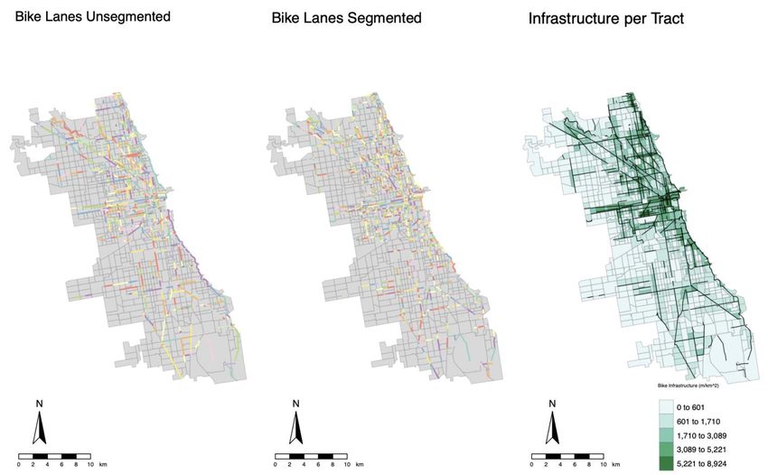
Table of Contents

Acknowledgements 04

Chapter 1
 Abstract 05
Chapter 2
 Introduction 06
Chapter 3
 Literature Review 09
Chapter 4
 Methods 16
Chapter 5
 Results 26
Chapter 6
 Discussion 35
Chapter 7
 Conclusion 41
Bibliography 42

Appendix A
 City Size and Region 48
Appendix B
 Classification of Tracts by City 50
Appendix C
 City Size and Region 52
Appendix D
 Percent Differences in Infrastructure by Tract Type 54
Appendix E
 Bike Infrastructure by Gentrification Status and City 56
Appendix F
 Mean Distance to CBD by Gent. Status and Results for Univariate Regression 59

 2

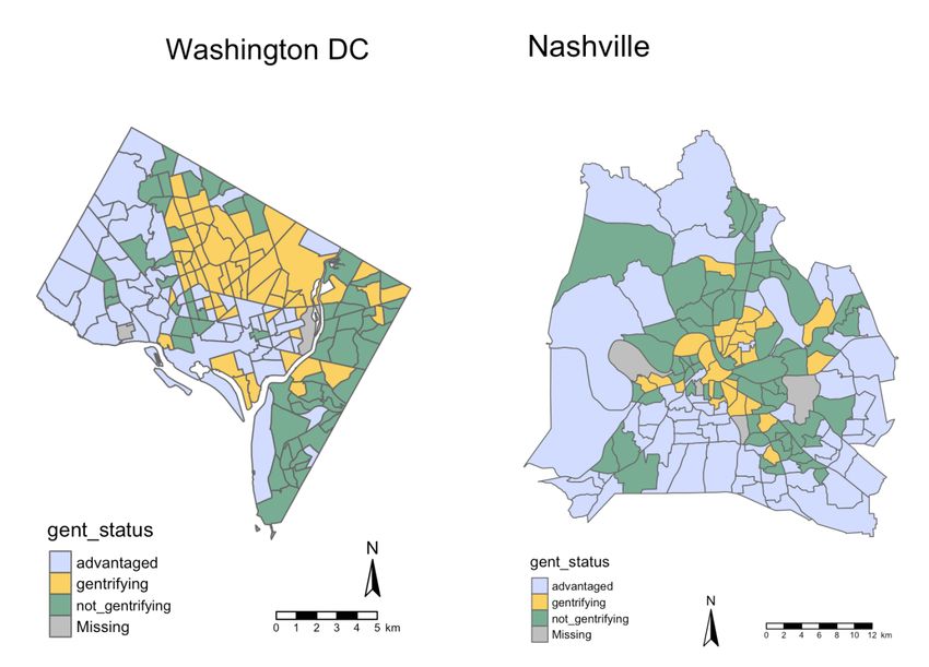
List of Figures

Fig. 1. Share of Commuters Who Cycle to Work (2016 ACS data) 10
Fig. 2. Freeman’s Gentrification Classification Scheme 20
Fig. 3. Assigning Bicycle Lane data to Census Tracts in Chicago 23
Fig. 4. Washington D.C. and Nashville Gentrification Status 26
Fig. 5. Washington D.C. and Nashville Bike Infrastructure 27
Fig. 6. Average Cycling Infrastructure by Lane or Trail Type 28
Fig. 7. Average Cycling Infrastructure by City Region in the US 29
Fig. 8. Average Cycling Infrastructure by City Size 30

 List of Tables

Table 1. Types of Bike Lanes 21
Table 2. Full Model Regression Results 31
Table 3. Regression Results by City Size 33
Table 4. Regression Results by Region 34

 3

Acknowledgements
 First, thank you to Professor Marynia Kolak. Professor Kolak served as the advisor for
this thesis. Through her GIS courses, Professor Kolak introduced me to conducting GIS in R and,
more generally, the open science paradigm which this project seeks to follow. Professor Kolak
provided crucial suggestions, continuous encouragement, opportunities to present and receive
feedback about this work, and connections to other researchers and spatial data professionals.
 Thank you also to Dr. Julia Koschinsky and Dylan Halpern at the Center for Spatial Data
Science. Both provided their time and advice. Dr. Koschinsky shared of her paper (Folch et al.
2014) which helped me decide on the spatial scale of the project, and Dylan was a good resource
for handling Open Street Map data which I considered using. I also appreciate the support of
Jamie Gentry who, along with Professor Kolak, has helped organize the Geography Major in the
past year and has put together events to support our writing of our thesis.
 Thank you to the numerous local and regional government officials who shared bicycle
infrastructure data and guidance on how to use it. Specifically, thank you Calley Mersmann (City
of Cleveland), Alex Rotenberry (Mid-America Regional Council), Maggie Green (City of
Kansas City), Jessica Buttermore (City of Memphis), Nicholas Oyler (City of Memphis), James
Hannig (City of Milwaukee), John Broome (City of Nashville), Marty Sewell (City of
Nashville), Jason Radinger (City of Nashville), David DosReis (City of Providence), and Josh
Lay (City of Washington DC).
 Finally, thanks to my family and friends for their support and willingness to listen to me
talk about gentrification and bike lanes this past year.
 Please note that though I received support from the above-mentioned individuals, any
errors in this thesis are only mine.

 4

Chapter 1

 Abstract

 In recent years, cities across the United States have expanded their bicycle infrastructure.
In some instances, community members and local politicians have criticized these developments
and noted a link between bicycle lanes and gentrification. In response, recent studies have
assessed the quantitative associations between bicycle infrastructure and gentrification in a few
large cities. Their results have been mixed but generally support residents’ claims of linkages
between gentrification and bike infrastructure. However, research is often limited to a handful of
large central cities, mostly in the United States.
 This thesis assessed the associations between gentrification and bicycle infrastructure
such as bike lanes and off-street trails and paths in 46 large American cities. Specifically, it used
contemporary municipal bicycle infrastructure data aggregated to the census tract level. It
conducted multivariate regression analyses to identify the cross-sectional associations between
gentrification and other socio-economic indicators and the presence of bike infrastructure. It
compared these associations by city size and geographic region. It found substantial evidence
that gentrifying tracts had higher rates of cycling infrastructure relative to disadvantaged, non-
gentrifying tracts. This trend was less pronounced in America’s largest 5 cities, and there was
substantial regional variation in both infrastructure coverage and relative levels when comparing
gentrifying, non-gentrifying, and advantaged tracts.

 5

Chapter 2

 Introduction

 Despite its widespread discussion within and outside academic literature, gentrification
lacks an agreed-upon definition. Scholars have associated the term with a transition from owning
to renting houses, a process of urban neighborhood “rediscovery,” a valorization of old buildings
and broader appreciation of urbanity relative to the suburban lifestyle, and the improvement of a
neighborhood’s infrastructure (Shaw, 2008). It is also associated with an urban, often minority,
neighborhood experiencing an influx of new capital, leisure activities, and residents of a higher
socioeconomic class and a different race, which is often White. This thesis uses Lance Freeman’s
(2005) conceptualization of gentrification which distinguishes gentrifying regions from
advantaged and not gentrifying (i.e. disadvantaged) ones based on their location in central cities,
median family income, recent housing development, change in housing prices, and change in
average levels of educational attainment. A more formal presentation of Freeman’s classification
can be found in the Methods section.
 Though scholars disagree on a definition, many recognize it has potentially substantial
negative consequences. Gentrification is commonly associated with displacement, or long-time
residents being forced out of a neighborhood due to increasing prices, in both academic
scholarship (Elliott-Cooper et al. 2020; Marcuse 1986; Shaw 2008) and popular media (Dragan
et al. 2019; Freeman 2005). Notably, when British sociologist Ruth Glass coined “gentrification”
in 1964, she contended that it led to price increases and social character changes that displaced
residents (Shaw 2008). Beyond displacement, gentrification can also restrict the range of
acceptable neighborhood behaviors, and gentrification can frustrate long-time community
members who feel slighted by their lack of input in neighborhood changes (Freeman, 2006, p.
196). These dynamics are more extensively discussed in the Literature Review.
 Critics of the development of cycling infrastructure in underserved neighborhoods make
arguments that fall in line with these more general concerns about gentrification. For example,
some residents and politicians of neighborhoods experiencing investments in bike infrastructure
also viewed this development as a potential cause of gentrification and displacement (Hoffmann,
2016; O’Sullivan, 2021; Kramer, 2020). Hoffman (2016) and Lubitow et al. (2016) documented

 6

how the development of bike lanes in minority neighborhoods in Portland and Chicago were
seen as symbols of gentrification and how the city government’s focus on this infrastructure
failed to respond to those communities’ wants and needs. This critique falls in line with the more
general notion that gentrifying neighborhoods fail to meet long-time residents’ desires. In short,
critics of the development of cycling infrastructure offer commentary that follows the broader
criticism of gentrification, a dynamic upon which I elaborate in the Literature Review.
 In this thesis, I assess the cross-sectional associations between gentrification and bicycle
lane development in 46 of the largest cities in the United States. This is both a gap in the
academic literature and a highly salient issue. Some recent studies (Flanagan et al., 2016; Braun,
2018) have conducted similar research on the association between cycling infrastructure and
gentrification, but their scope has only included a handful of major cities like Chicago, Portland,
Oakland, and Minneapolis. This scope is limited, so the extent to which gentrification and
cycling lanes co-occur across large cities in the United States remains unclear. Moreover, as
discussed above, the co-occurrence of gentrification and the development of cycling
infrastructure can be fraught and incredibly frustrating to local residents, making it salient even if
the causal relationship between cycling lanes and gentrification remains unclear (Hoffman, 2016;
Lubitow et al., 2016). This research is also relevant from an equity-oriented perspective because
it compares presence of a public amenity across different communities in large American cities.
Thus, it is important to study these associations at a broader scale across the United States.
 Following Braun (2018), I used 2015-2019 American Community Survey data to assess
whether a specific census tract was gentrifying. I collected municipal-level spatial bicycle
infrastructure data from 2015 onward in each of the cities studied and used multi-variate
Ordinary Least Squares (OLS) regressions to assess the associations between census tracts’
gentrification status and their level of bicycle infrastructure, as measured by distance of bicycle
lanes or off-road trails per square kilometer. I controlled for distance to the central business
district, population density, and number of young residents, all potential predictors of cycling
infrastructure, and also added a term for the number of minority residents in the region. I then
compared similar models for cities of different sizes and in different regions of the United States.
 The results suggest that there is substantial spatial heterogeneity in the distribution of
census tracts in major American cities. Overall, gentrifying tracts tend to have greater levels of
cycling infrastructure than both advantaged and not gentrifying tracts. When controlling for other

 7

factors, gentrifying tracts still have on average higher levels of cycling infrastructure relative to
not gentrifying tracts, but no statistically significant differences with advantaged tracts. When
considering cities by size, extremely large cities (MSA population > 7 million) tend to have less
infrastructure than other cities. When considering cities by region and controlling for other
factors, non-gentrifying tracts in the Interior West and South have statistically significantly lower
rates of cycling infrastructure.
 This research built upon the existing literature on bicycle infrastructure and
gentrification. Specifically, it supported the findings of Braun (2018), Tucker and Manaugh
(2018), and Flanagan et al. (2016) by documenting the inequitable distribution of bicycle
infrastructure by race and by neighborhood gentrification status. Notably, these findings contrast
with those of Houde et al. (2018) who studied Montreal and the surrounding region. The results
also advanced the qualitative literature and media reports’ identification of cases in which
gentrification and bicycle infrastructure development co-occur by assessing the scope of this
issue in major metropolises across the United States.

 8

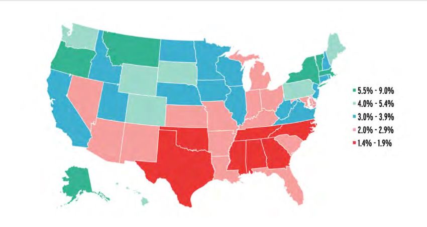
Chapter 3

 Literature Review

 This literature review aims to delve further into the issues discussed in the Introduction.
Specifically, it will begin by describing cycling trends in the United States and the process by
which new cycling lanes are allocated. It subsequently deepens the discussion about the
consequences of gentrification by considering both displacement and other issues. It provides a
broader context to criticism of bike lanes in conjunction with gentrification by discussing New
Urbanism and “the creative class.” This discussion serves to contextualize criticisms of the
development of cycling infrastructure which I consider more in depth here.

Bicycling in the United States
 While bicycling in the America in the last decade has served as a relatively steady source
of transportation, rates of cycling tend to be broken down by demography and geography.
National Household Travel Survey (NHTS) data suggest that between 2009 and 2017, about 1%
of all trips were taken by bicycle. This same data finds that women are under-represented as
cyclists, making up only 28.0% of bicycle commuters. Data from the 2005 to 2016 American
Community Surveys (ACS) suggests that about 0.5% of all commutes are taken by bike. 2008-
2012 ACS data indicates an inverse relationship between income and bicycling; about 1.5% of
commuters earning less than $10,000 biked to work, whereas only about 0.5% of workers
earning greater than $200,000 cycled to work during the same time. While the 2010 Decennial
Census suggests that about 28% of Americans are non-White, only about 20% of bicycle trips
were made by cyclists of color based 2009 and 2017 NHTS data. Southern states make up eight
of the ten states with the lowest rates of cycling to work, demonstrating spatial heterogeneity in
rates of cycling as a mode of transportation (see Figure 1) (McLeod et al., 2018). In short,
cycling rates vary across the country, White people tend to cycle more, and extremely high
earners commute by bike less.

 9

Bike Lane Distribution:
 At least three theories explain the distribution of the development of bicycle lanes in the
United States. First, bicycle infrastructure could follow, and potentially be caused by, a region
becoming more socio-demographically advantaged (Braun, 2018). This theory is consistent with
findings that urban planning and infrastructure development responds to the desires of
advantaged, often White, residents (Hoffmann, 2016; Braun, 2018). Second, bicycle
infrastructure development could precede, and potentially induce a neighborhood to experience
an influx of advantaged residents (Braun, 2018). This follows Richard Florida’s prescription of
developing successful cities by attracting well-educated white-collar workers with urban
amenities like cycling lanes (Florida 2002; Braun, 2018). Finally, bicycle infrastructure could
develop as a consequence of more “traditional” demand factors that depend upon urban form and
demographics like high percentages of young residents, population density, and proximity to a
city’s urban core (Braun, 2018).

Figure 1: Share of Commuters who cycle to work (2016 ACS data)

From McLeod et al., 2018, page 215

 10

Gentrification and Displacement

 The causal relationship between gentrification and displacement has been hotly contested
in academic planning and sociological literatures. Some scholars find gentrification does not
generally cause displacement (Henig, 1980; Vigdor, 2002; Freeman and Braconi, 2004; Dragan
et al., 2019). However, much of this research has been criticized (Slater 2009; Newman and
Wyly, 2006; Marcuse, 2005). Other scholarship has found statistically significant, if relatively
small in magnitude, evidence of gentrification-induced displacement, particularly in more recent
years (Newman and Wyly, 2006; Brummet and Reed, 2019; Owen, 2012). Finally, other research
takes a different stance on the issue, suggesting that there is no causal relationship except in
major cities like London (Freeman et al., 2016), that displacement can be an antecedent to
gentrification (Billingham, 2017), or that concentrated poverty, not gentrification-induced
displacement, is crucial to study when seeking to ameliorate the plight of the urban poor
(Cortwright & Mahmoudi, 2014).

Other Impacts of Gentrification:
 Despite quantitative social science’s mixed record definitively identifying gentrification
as a major driver of displacement, the literature recognizes the harms of gentrification and
displacement. Elliott-Cooper et al. (2020) eloquently argued that displacement is a form of
systematic violence that can lead to psychological and even post-traumatic stress. Freeman,
(2006) classified gentrification as "repressive and restrictive." In two historically Black New
York neighborhoods, he specifically noted that activities like congregating on street corners,
barbequing in parks, and publicly consuming alcohol became unacceptable as the neighborhoods
underwent gentrification (Freeman, 2006, 196). Freeman (2006) also described “the specter of
displacement,” observing that the fear of displacement was also harmful to gentrifying
neighborhoods, regardless of whether displacement actually occurred (p. 162-164).
Neighborhood changes associated with gentrification also frustrated some long-time residents
who were perturbed by their lack of control over their community (Lubitow et al., 2016;
Tavernise, 2011; Badger, 2020; Mirk, 2012).
 Even so, gentrification does bring some benefits. Theoretically, it can mitigate
segregation by allowing the mixing of races and classes (Newman & Wyly, 2006). Relatedly, it
can allow middle class Blacks to live in middle-class neighborhoods rather than being forced to

 11

choose between well-off White or disinvested Black communities (Freeman, 2006, p. 197). It
can also allow low-income children in poorer families who remain in gentrifying neighborhoods
to experience major positive educational and professional outcomes (Chetty et al., 2016; Dragan
et al., 2020). Residents in gentrifying neighborhoods, particularly in those that had been
extremely disinvested, likely also experience increasing access to neighborhood services and
amenities (Freeman, 2006, p. 160). In other words, gentrification has some potentially positive
outcomes.

Theoretical Foundations: New Urbanism and the “Creative Class”

 New Urbanism and the notion of the “creative class” support bike infrastructure
development in cities. However, both philosophies have been criticized for their lack of equity in
general and, specifically, with respect to bike lanes.
 New Urbanism supports sustainable, mixed-use urban form and is supportive of bike
infrastructure. Generally, New Urbanism encourages neighborhoods with compact form, close
proximity between jobs and residences, decreased usage of cars, and the fostering of unique
neighborhood identities (Day, 2003; Grant, 2011). The Charter of the New Urbanism encourages
the creation of bicycle networks to reduce car usage (Congress for the New Urbanism, 2000).
New Urbanism is important in practice; New Urbanist ideas were crucial to the Department of
Housing and Urban Development’s Hope VI program as well as the plans and regulatory codes
of numerous cities across the United States (Bohl, 2000).
 New Urbanism broadly has come under fire for equity-related issues. New Urbanist
scholar Emily Talen wrote that neighborhoods that subscribe to Jane Jacobs’s tenets, which
served as part of the inspiration for New Urbanism, can experience gentrification and
displacement and that physical urban development needs to be partnered with anti-displacement
policy (Talen, 2012). Day (2003) and Larsen (2005) echoed this argument, contending that the
New Urbanist “toolkit” relies almost exclusively on physical changes to the built environment
and is, therefore, less responsive to communities’ other concerns. Finally, New Urbanists’
traditional modes of community engagement may not be tailored for communities considering
neighborhood changes (Day, 2003). In other words, critiques of New Urbanism have pointed to
the fact that its neighborhood improvements can lead to displacement, may not respond to

 12

existing community-members’ most pressing needs, and could fail to engage the community
effectively.
 The conception of the “creative class” presents another modern and influential view of
successful cities and encourages bike infrastructure. In his 2002 book The Rise of the Creative
Class, Richard Florida defined the “creative class” as people with jobs that are not blue collar, in
the service industry, or agriculture-related (2002, p. 328). Florida contended that the creative
class fuels economic growth, so cities should seek to attract them with retail and entertainment
amenities (2002, 223-232, 249-250). Florida also identified the creative class’s strong association
with bicycling (2002, p. 172-173, 181-182). Ideas about the “creative cities” have strongly
influenced policy-decisions in many major cities including London, Tampa Bay, Silicon Valley,
Auckland, and Brisbane (Atkinson & Easthope, 2009).
 Florida’s concepts have been strongly criticized, in part for equity-related issues. Edward
Glaeser analyzed Florida’s own data and concluded that his policy prescriptions are
unsubstantiated (Glaeser, n.d.). Florida himself acknowledges that creating places attractive to
the “creative class” could raise housing costs (Peck, 2005). Moreover, meeting the needs of the
“creative class” could simultaneously expand the poorly paid service industry who would
respond to “creatives’” desires (Peck 2005). Wilson & Keil (2008) came to similar conclusions,
arguing that Florida’s ideas only act as a new rationale to encourage public policies that privilege
the elite. They added that they ignore cities’ true problems: inequality, segregation, and unstable
economies (Wilson & Keil, 2008). In sum, Florida’s (2002) ideas have been criticized
methodologically and substantively for their potential to cause displacement and for their lack of
consideration of the poor.

New Urbanism, the Creative Class, and Bicycle Infrastructure
 The broad critiques of New Urbanism and tailoring to the “creative class” apply
specifically to the development of bicycle infrastructure. Former Chicago Mayor Rahm
Emmanuel’s $150 million plan to improve Chicago’s bike infrastructure was criticized for the
city’s not consulting communities in which the new bike lanes were to be built (Lepeska, 2011).
Then Mayor Emanuel pitched this development as a way to attract new tech companies and start-
ups, an almost explicit allusion to Florida’s “creative class” (Lubitow et al., 2016). Some Black
residents in a historically minority and underserved but gentrifying neighborhood in Portland

 13

contended that the city only invested in the neighborhood when White people relocated there
(Hoffmann, 2016; Davis, 2011; Goodyear, 2011). Hoffman (2016) observed that the
development did not respond to the needs of long-term residents, one reason why bike lanes
antagonized the community. Since the onset of the global COVID-19 pandemic, a number of
large cities have transformed their urban spaces, including creating slow streets that are bikeable
and planning new bike lanes, but this rapid urban change often has not included the desires of
marginalized residents (Kramer, 2020; Badger, 2020). In short, the development of new bike
lanes has been criticized for not consulting underprivileged residents, failing to consider their
wants and needs, and potentially inducing gentrification and displacement.

Bike Lane Criticism and Association with Gentrification

 In the past decade and, in particular, since the onset of the pandemic, local politicians and
community members in major cities across the United States have criticized bike infrastructure
development for its potential to cause gentrification and displacement. A 2011 New York Times
article reported that some poorer residents of Washington D.C. saw the city’s revitalization,
which included building bike lanes, as “code for efforts to drive them out” (Tavernise, 2011).
Some local Portland communities reportedly called the development of new bike lanes through a
historically marginalized and minority community “white stripes of gentrification” (Davis,
2011). At the CityLab 2021 Conference, urban designer Jay Pitter argued that marginalized
communities resist bike lane development because they “spur gentrification” (O’Sullivan, 2021).
In Washington D.C., Ward 8 Councilmember Trayon White argued that new bike lanes “force
aspects of gentrification and displacement” (Kramer, 2020). In other words, politicians and
community members have also criticized bike lane development and argued that it is associated
with gentrification.

Quantitative Studies Assessing Equity and Bike Infrastructure

 While a relatively new sub-field, four recent studies have assessed various aspects of bike
infrastructure and their associations with gentrification, generally finding some small but
significant positive correlations. In a longitudinal study with data from 1990 to 2015, Braun
(2018) studied Chicago, Minneapolis, and Oakland. In Chicago and Oakland, Braun (2018)
found associations between bike infrastructure and areas that were either advantaged or

 14

gentrifying (as opposed to those that were disadvantaged). The results in Minneapolis were more
mixed, but the overall evidence supported the linkage between bike lanes and gentrification
(Braun, 2018). When running lagged regressions, Braun (2018) found that gentrification
preceded bike infrastructure in Chicago, and gentrification and bike lane development occurred
at the same time in Oakland. Flanagan et al. (2016) studied bike infrastructure, including
inexpensive bicycle share stations, in Chicago and Portland from 1990 to 2010, concluding that
bike infrastructure tended to be invested in gentrifying or privileged areas. In Montreal and two
neighboring cities, Houde et al. (2018) found that lower-income residents have notably good
access to bicycle infrastructure and that this infrastructure was increasingly accessible to
immigrants. However, in Rio de Janeiro and Curitiba, Brazil, bicycle infrastructure was highly
concentrated in wealthy areas (Tucker & Manaugh, 2018). In short, in recent years, a handful of
quantitative studies have begun to document associations between bike lanes and privilege and
generally, but not exclusively, find positive associations.
 Other studies have considered the disparities in distribution of bike lanes in major
American cities along other lines. For example, Braun (2018) also collected spatial data on
bicycle infrastructure in 22 major American cities and used regressions to assess the extent to
which socioeconomic indicators were associated with greater bicycle infrastructure. She
controlled for population and employment density, distance to a central business district, young
residents, and commuters who used a bicycle. She found associations between less bicycle
infrastructure and some indicators of disadvantage, like lower educational attainment and higher
proportions of Hispanic residents, but not with others, such as lower income, higher poverty, and
proportions of Black residents. Hirsch et al. (2017) studied the clustering of bicycle lanes and
trails, as well as bus transit services and parks, in Birmingham, Minneapolis, Oakland, and
Chicago, finding associations between the construction of bike lanes and falling unemployment.
Hirsch et al. (2017) also found some evidence of clustering in the development of bike lanes in
dense urban areas while paths and trails tended to see increased development in the periphery of
the cities in their study.

 15

Chapter 4

 Methods

 This section is divided into seven distinct subsections. The first considers the selection
process for the 46 cities included in this thesis, the decision to use the census tract as the unit of
spatial analysis, and the methods utilized to select census tracts for each of those cities. The
second considers the spatial and temporal scope of the project. The third presents Freeman’s
(2005) gentrification classification scheme and how I applied it to more recent and slightly
different data. The fourth and fifth describe the processes of collecting and handling other
covariate data and cycling lane spatial data. The sixth presents my cleaning and aggregation of
the cycling lane data. The last subsection describes the analysis process. Also, note that all work
was conducted in R.1

City Selection and Classification:

 I limited this study to considering central cities for two reasons. First, Freeman’s (2005)
gentrification indicator identified tracts as gentrifying only if they reside in a central city. This
will be discussed more fully later in the gentrification subsection. Second, many suburban
municipalities did not have publicly available cycling data, and the task of collecting cycling
data from many suburban municipalities would have been too time-intensive for the scope of this
work. I also limited the central cities in consideration to those in Metropolitan Statistical Areas
(MSAs) with populations greater than 1 million according to 2019 1-year ACS data. This cutoff
is somewhat arbitrary but necessary to capture the dynamics in cities rather than towns. I filtered
out the eight cities which met this population criterion but whose bicycle data I could not find.
The search for bike lane data is described later in this section. I also removed Tucson, AZ due to
its bicycle data being from 2014, before the start of the five-year ACS estimates I used to classify
the tracts as gentrifying (see the gentrification subsection). This left 46 cities.

1
 Scripts can be found here: https://github.com/Deckart2/bikes_thesis

 16

I classified each of these 46 cities by size and region. I divided cities into three groups
based on their 2019 1-year MSA population. I classified cities in MSAs with > 7 million people
as “extremely large cities," 3-7 million as “large cities,” and < 3 million as “medium cities.” I
also classified the cities into one of five geographic regions in the US: West Coast, South,
Southwest, North East, and Midwest. The cities and their size and region can be seen in
Appendix A.

Spatial and Temporal Scope:

 I used census tracts as the unit of analysis. This followed Flanagan et al. (2016). Notably
Braun (2018) used the smaller block groups which theoretically gave more resolution to the data.
However, when considering the spatial scale, I followed Folch et al.'s (2014) suggestion to
consider the coefficient of variation (CV), an estimate’s standard error divided by the estimate
itself. Many estimates had CVs of either “medium reliability” (between .12 and .40) or worse
(greater than .40) at the block group level, leading me to choose to use the census tract level
(Folch et al., 2014).

 I used geo-computational methods to select each city’s census tracts. I began with a
shapefile with 2010 census tract boundaries for the entire US from IPUMS. For each of the 46
cities studied, I downloaded a polygon spatial data layer to identify city limits. Many cities had
explicit datasets for city boundaries but when those were unavailable, I downloaded other
polygon datasets, like, for example, city councilmembers’ districts, which covered the extent of
the city.2 I then performed spatial unions on each of the 46 cities’ polygon datasets to convert
those datasets into a single multi-polygon layer. I joined all cities’ boundaries into one dataframe
and buffered each by 125 meters, selected all census tracts strictly within the buffered city
boundaries, and assigned those tracts to their respective city. 125 meters was chosen because it
effectively selected the census tracts of representative cities Chicago, Washington D.C. and
Portland. Once filtering the census tracts to include only those in the cities of interest, I joined
that data to the non-spatial ACS data.

 I used this method for two reasons. First, city data portals did not uniformly report the
census tracts in their city, so I wanted to use a more universal selection method. Second,

2
 The specific sources of this data can be found here: https://tinyurl.com/morrisonthesis

 17

performing selection using intersects methods (i.e. st_intersects in R’s sf package’s parlance)
identified census tracts largely outside of city boundaries but with small portions of overlap
inside the boundaries.

 This thesis solely focuses on cross-temporal associations. As noted above, I use only
cycling data from 2015 onwards. Additionally, the gentrification index, discussed more fully
below, classifies tracts using ACS data from 2015-2019.

Gentrification:

 To identify gentrifying tracts, I generally followed Braun (2018) in using Freeman’s
(2005) method. Freeman considered two years 10 years apart3 and used five criteria to classify a
tract as gentrifying. These were that the census tract:

 1. Was located in the central city of a region
 2. Had a median family income less than the MSA’s median family income in the first year
 3. Had a proportion of housing stock built in the 20 years preceding the first year lower than
 the median proportion of housing stock built for the MSA during those same 20 years
 4. Had an increase in percentage of residents ages 25 or more with a bachelor’s degrees that
 was higher than the rise in the MSA’s percent increase in residents ages 25 or more with
 bachelors degrees in the ten-year time period
 5. Had a real increase in housing prices in the ten-year time period

 All tracts considered in this study meet the first criterion. If a tract did not meet either of
the second or third criteria, it was classified as “advantaged” and, therefore, ineligible to gentrify.
Tracts that met the first three criteria but not the last two were called “not gentrifying,” and only
tracts that met all criteria were deemed “gentrifying.” While I use the descriptor “not
gentrifying,” these tracts should be considered disadvantaged regions in their cities given that
they had some combination of low median family incomes, housing investment, increases in
educational attainment and increases in housing prices.

3
 The 10 year separation comes from Freeman’s usage of the census.

 18

It should be noted that my measure of gentrification varies slightly from Freeman’s in
that he uses Decennial Census data which has a 10-year interval, and this thesis’s 2006-2010 and
2015-2019 5-year ACS estimates have a slightly shorter interval of effectively 9 years. I used
2015-2019 data because it is the most recently updated ACS data available at the time of writing
this thesis. While 2005-2009 ACS data exists, NHGIS noted that “no TIGER/Line files represent
the actual set of tracts… identified in 2005-2009 ACS tables, so NHGIS does not provide
boundary files for the ‘2009 vintage’ of these results” (goray). To avoid addressing this issue and
the potential errors associated with cross-walking data from 2000 to 2010 census tracts, I used
2006-2010 data which, like the 2015-2019 data, exists at the 2010 census tract scale.

 Figure 2 illustrates the process of classifying tracts as gentrifying, advantaged, and not
gentrifying. Appendix B lists the number of tracts in each city that are gentrifying, advantaged,
and not gentrifying.

 Covariates:

 I collected covariate data from two types of sources: an aggregated city center dataset
created by Holian (2019)4 and the 2015-2019 ACS.

 From the 2015-2019 ACS, I also collected covariate data on the number of minority
residents (i.e. all of those who were not classified as non-Hispanic White), total population, and
total population ages 18-34. I divided the total population by the area of the census tract to
compute population density.

 Holian (2019) studied and aggregated different central business district (CBD) datasets.
Notably, 1982 Census researchers identified CBDs in 385 cities, and researchers from the
Federal Reserve (Fee & Hartley, 2012) converted more than 200 of those areas into points. For
central cities not included in this study, Holian (2019) noted that one available alternative is
using the city hall’s geocoded location from an ArcGIS dataset that he also provided. Holian
shared this data, as well as other identifications of CBDs, on his blog. For the 46 cities
considered in this thesis, I use the point identified by Fee & Hartley (2012) if it existed or,
otherwise, the ArcGIS geocoded city hall location. Saint Paul’s city hall was not in either dataset,
so I used Google Maps to identify the latitude and longitude of its city hall and inputted it

4
 Data downloaded here: http://mattholian.blogspot.com/2013/05/central-business-district-geocodes.html

 19

manually. I then computed the distance between the centroid of each census tract and the point
identified as the city center.

 In summary, from Holian (2019) and the 2015-2019 ACS, I collected the following
covariate measures: population density, population ages 18-34, distance to CBD, and number of
minority residents.

Figure 2: Freeman’s gentrification classification scheme

This chart modifies chart 4.2 1 from Braun (2018).

 20

Bike Lane Data Geo-computation:

 To gather information on each city’s bicycle paths and trails, I first sought to find the
spatial bike lane data via each city’s website. Many large cities had open data portals with bike
lanes and trails as unique spatial datasets (i.e. Shapefiles and more occasionally GeoJSON and
Geodatabases with “linestring” or “multi-linestring” data indicating the location of bicycle lanes
and paths). If I could not find such data, I sought similar or related data from larger government
entities like counties and states. For example, to identify bicycle paths and routes for Salt Lake
City, I downloaded Utah’s road and trail data separately. Their road data noted whether a road
had a bike lane, and their trail data denoted the type of path of interest. If I could not find data
from a larger municipal entity, I reached out to city agencies requesting their data. Some cities
had formal data request processes while, for others, I emailed representatives from the
Departments of Planning, Transportation, or Engineering. Ultimately, through this process, I
collected data from 46 cities. It should be noted that while I was unsuccessful in my attempt to
collect data from 7 other cities, that data likely exists and very well could be publicly available; I
was simply unable to find it or reach out to the correct city department or regional agency.

Table 1: Types of Bike Lanes

 Type Description:

 Separated trails and paths Paved or compact paths not on roads that tend to be multi-use
 and that bikers can use.

 Protected bike lanes On-street lanes with physical barriers separating the bike and
 car lanes.

 Bike lanes A designated, painted lane for bikers without physical barriers
 between car and bike lanes.

 Shared lanes Portions of the road designated for bikers to use but which
 other vehicles, either buses or sometimes cars and buses, may
 also use. This classification includes “sharrows.”

 Bike boulevards Streets with physical infrastructure to slow traffic speeds but
 that lack “regular” bike lanes.

 21

Cleaning the bike lane data was a heterogeneous process since each file had a separate
structure. However, the general process involved selecting existing attributes to avoid including
lanes that were planned to be built in the future. I also converted all shapefiles to a standard
coordinate reference system (ESPG 2163). If the data source permitted, I grouped the bike lane
data into one of five categories whose general descriptions are in Table 1. Again, due to the
heterogeneity of data and the general lack of metadata, cities’ descriptions of their bike
infrastructure varied. Some cities had far more than these five bike lane categories, while others
had less. Consequently, while the descriptions constitute a “best guess” for a unified
classification scheme, such disparate data is inherently inconsistent. When I could not ascertain
the type of infrastructure, I classified the type as “unknown.” To aggregate the bike infrastructure
data to the tract level, I first split all of the bike lane line data so that each segment was located in
exactly one census tract. I then computed the distance of the lane. Finally, I standardized the data
in each tract by dividing the total distance and distance of each lane type for all line segments by
the area of the tract. This process can be seen in Figure 3. The first panel shows Chicago’s
census tracts and bike infrastructure relatively unprocessed. The second shows the bicycle
infrastructure subdivided by the census tracts; this is perhaps most easily apparent in the southern
portion of Chicago. The third panel shows the level of cycling infrastructure in each tract in units
of meters of bicycle infrastructure per square kilometer in each census tract. The full lanes are
also overlaid above the census tracts in the third panel.

Statistical Analysis

 The dependent variables in this study were measures of bicycle infrastructure per census
tract and in units of / 2 , as described above. Dividing the distance of bike infrastructure by
tract area responded to the modifiable areal unit problem. That is, without dividing by the area,
tracts with larger areas would likely have had more bicycle infrastructure. Most of the t-tests and
regressions conducted used the total bicycle infrastructure, the sum of all of the categories
described in Table 1, but some considered each of the types separately.

 22

Figure 3: Assigning Bicycle Lane data to Census Tracts in Chicago

 I first computed the level of bike infrastructure in / 2 in the census tract for all bike
infrastructure and for each bicycle type (see Figure 6). I then conducted pairwise t-tests to assess
whether the mean bicycle infrastructure measure in gentrifying, advantaged, and not gentrifying
tracts were the same (see Appendix C). Specifically, I used a two-sided t-test that did not pool
standard deviations or assume equal variance among groups. I used Bonferroni’s method to
control for conducting three tests and used a 95% confidence level. I conducted a similar analysis
but with Holm’s method and considered the cities by geographic region and size (Figure 7 and
Appendix C, Figure 8 and Appendix C). Finally, I computed the percent difference between
gentrifying and advantaged and gentrifying and not gentrifying tracts for each city and then
plotted those values by city (see Appendix D).

 I created an OLS multi-variate regression model in R considering all of the tracts across
all cities studied (Equation 1). For each variable in the equation, i represents the i-th tract and j

 23

indicates the j-th city. The dependent variable was the measure of total cycling infrastructure (in
 / 2 ), following Braun (2018). This is indicated as , . The independent variables
were two dummy variables representing the gentrification status. _ , takes on 1 when
the tract is neither advantaged nor not gentrifying and 0 when it is gentrifying. , 
takes on 1 when the tract is advantaged and 0 when it is gentrifying; thus, gentrifying tracts were
the “base case” to which advantaged and non-gentrifying tracts were compared. The fourth
through sixth terms of the equation represent control variables. These constitute what Braun
(2018) classified as “objective demand factors,” or urban form or demographic characteristics of
regions that make them conducive to cycling. Specifically, they are population density, distance
to the CBD, and number of residents ages 18-34. Dense areas near the CBD often are viewed as
having higher demand for cycling, and young people (i.e. those 18-34) tend to cycle more
(Braun, 2018). Braun (2018) and Flanagan et al. (2016) use all of these measures in their
regression analysis; Braun (2018) used all three as controls and Flanagan et al. (2016) used two
of the three as controls but number of young residents as part of their own gentrification index.
Houde et al. (2018) included distance to the central business district as a control. I included a
measure for the number of minority residents to capture an aspect of gentrification not included
in Freeman’s (2005) analysis. Finally, I again followed Braun (2018) in including dummy
variables for each city. This is represented by . This allowed the regression to assume different
baseline levels of cycling infrastructure for each city.

Equation 1:

 , = β0 + β1 _ , + β2 , + β3 _ , + β4 _ _ , 
 + β5 _18_34 , + β6 , + + ϵi,j

 I also ran a number of smaller models on different subsets of cities by city region and
size. These models looked similar to the model specification described above with the exception
that I removed dummy variables; also, these models were applied to specific subsets of the data.
This specification is shown in Equation 2.

 24

Equation 2:

 = β0 + β1 _ + β2 + β3 _ + β4 _ _ 
 + β5 _18_34 + β6 + ϵi

 25

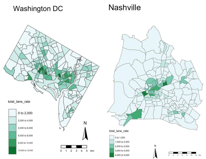
Chapter 5

 Results

Visualization of Findings:

 Figure 4 illustrates how Freeman’s (2005) index classifies the tracts in Washington D.C.
and Nashville, Tennessee. Figure 5 shows the bicycle infrastructure measure. These cities are
shown solely for demonstrative purposes to illustrate the results of the methods described in the
previous section.

Figure 4: Washington D.C. and Nashville Gentrification Status

 26

Figure 5: Washington DC and Nashville Bike Infrastructure ( / )

Statistical Tests Comparing Means:

 Assessing the overall levels of bicycle infrastructure in the tracts by gentrification
classification, the general trend was that gentrifying tracts had higher rates of infrastructure than
advantaged tracts and not gentrifying tracts. This relationship was statistically significant (p

by cycling infrastructure type, city size, and city region and the significance levels of the
differences between the three tract types are reported in Appendix C. Additionally, the level of
cycling infrastructure in each tract type for each individual city can be found in Appendix E.

Figure 6: Average Cycling Infrastructure by Lane or Trail Type

 Average Cycling Infrastructure by Type
 2000

 1500
 Bike Infrastructure m/km^2

 gent_status
 Advantaged
 1000
 Gentrifying
 Not Gentrifying

 500

 0

 Bike Boulevard Protected Lane Regular Separated Trail/Path Shared Lane Total
 Lane Type

 Analyzing bicycle infrastructure by gentrification status and city region was more
ambiguous. Cities in the Midwest and on the West Coast had substantially higher rates of cycling
infrastructure in all three gentrifying groups relative to the other three regions. Among the three
groups of tracts, gentrifying regions in both the Midwest and West Coast had the highest rates of
cycling infrastructure, and the differences between advantaged and not-gentrifying tracts was not
statistically significant. Cities in the South, Northeast and Interior West all had lower overall
rates of cycling infrastructure, and all differences were statistically significant, suggesting greater
disparities in cycling infrastructure. In those three regions, gentrifying tracts had higher rates of
cycling infrastructure relative to not gentrifying and advantaged tracts. In the Interior West and

 28

South, advantaged tracts had higher rates of cycling infrastructure than non-gentrifying tracts,
but in the Northeast, non-gentrifying tracts had higher rates of cycling infrastructure.

Figure 7: Average Cycling Infrastructure by City’s Region in the US
 Average Cycling Infrastructure by Region
 Bike Infrastructure m/km^2

 2000

 gent_status
 Advantaged
 Gentrifying
 Not Gentrifying
 1000

 0

 Interior West Midwest Northeast South West Coast
 City Region

 Extremely large cities had higher rates of cycling infrastructure in advantaged and not
gentrifying tracts relative to gentrifying tracts, but far lower rates on the whole compared with
medium and large cities. In extremely large cities, there was no statistically significant difference
in the cycling infrastructure in each of the three groups. In large cities, gentrifying tracts had
higher rates of cycling infrastructure relative to advantaged tracts, and advantaged tracts had
higher rates of cycling infrastructure relative to non-gentrifying tracts. In medium-sized cities,
gentrifying tracts also had the highest rates of cycling infrastructure, but non-gentrifying tracts
had higher rates of infrastructure than advantaged tracts.

 Appendix D visualizes the percent difference when comparing the level of cycling
infrastructure in gentrifying tracts to not gentrifying or advantaged tracts. These were calculated

 29

by taking the difference in infrastructure rates in gentrifying and the other tract type of tract and
dividing by the level of infrastructure in the gentrifying tract. Both charts’ bars are colored by the
city size. Numbers close to 1 indicate that gentrifying tracts had substantially higher levels of
cycling infrastructure relative to the other group. Numbers close to 0 indicate relative
equivalence between the two groups, and negative numbers indicate that the tract type to which
gentrifying tracts were compared had higher rates of cycling infrastructure in that city. In both
charts, the two extreme negative values come from Hartford, CT and Miami, FL. According to
the data collected I collected, Hartford lacked cycling infrastructure in gentrifying tracts entirely,
and Miami had extremely low levels of cycling infrastructure in gentrifying tracts. More broadly,
however, in both charts, the wide range of values suggested that cities were relatively
heterogeneous in relative cycling infrastructure allocation among the three tract types. From the
comparison between gentrifying and advantaged tracts, medium cities tended to have higher
levels of cycling infrastructure relative to large and extremely large cities, but this trend was not
as readily apparent in the other chart.

Figure 8: Average Level of Cycling Infrastructure by City Size

 Average Cycling Infrastructure by City Size
 Bike Infrastructure m/km^2

 2000

 gent_status
 Advantaged
 Gentrifying
 Not Gentrifying
 1000

 0

 Extremely Large Large Medium
 City Size

 30

Regression Analysis:
 The “full model” described above (see Table 2) used data from all cities. As noted above,
the unit of analysis was the census tract, and the dependent variable was meters of bicycle
infrastructure per square kilometer. The predictor variables are the Euclidian distance from the
centroid of the census tract to the city’s CBD, the population density, total population ages 18-34
as of 2019, the total minority population in 2019, a dummy variable for each city, and two
dummy variables indicating whether the tract was advantaged, not gentrifying, or gentrifying.
The last two dummy variables serve as the independent variables while the other variables
controlled for urban form-related factors that external to gentrification could predict cycling
infrastructure. Note that due to this specification, gentrification was the baseline to which non-
gentrifying and advantaged tracts were compared. I also ran similar models considering each city
by region (Table 6) and by city size (Table 7).

Table 2: Full Model Regression Results 5

 total_lane_rate
is_not_gentrifying -131.187** (56.534)
is_advantaged -79.569 (55.548)
dist_to_cbd_km -42.673*** (2.461)
pop_density 0.006*** (0.002)
pop_18_34_2019 0.400*** (0.023)
minority_2019 -0.169*** (0.011)
Constant 935.806*** (143.537)
N 10,882
R2 0.665
Adjusted R2 0.663
Residual Std. Error 1,447.188 (df = 10830)
F Statistic 420.974*** (df = 51; 10830)
 ***p
Note: < .01; **p < .05; *p < .1
 The results demonstrated that gentrifying tracts have statistically significantly (p

variables were all meaningful predictors of cycling infrastructure. Specifically, when controlling
for the other factors in the model, on average gentrifying tracts had about 131 / 2 more
cycling infrastructure than non-gentrifying tracts. The difference between gentrifying and
advantaged tracts was not statistically significant. Each of the predictors were strongly
statistically significant (p

Medium Large Extremely Large
is_not_gentrifying 254.932 (169.437) -50.939 (155.064) 137.578* (77.795)
is_advantaged 361.072** (171.080) 748.356*** (153.313) 24.952 (74.150)
 *** ***
dist_to_cbd_km -98.492 (10.434) -88.620 (8.068) -11.226*** (2.233)
pop_density 0.602*** (0.030) 0.153*** (0.009) -0.018*** (0.001)
pop_18_34_2019 -0.017 (0.076) 0.371*** (0.057) 0.409*** (0.028)
minority_2019 -0.269*** (0.036) -0.162*** (0.030) -0.103*** (0.011)
Constant 1,813.829*** (188.579) 1,780.332*** (170.270) 700.285*** (81.922)
N 3,859 2,415 4,608
 2
R 0.176 0.273 0.078
Adjusted R2 0.175 0.271 0.077
Residual Std. Error 2,923.187 (df = 3852) 2,148.448 (df = 2408) 1,068.393 (df = 4601)
F Statistic 137.123 (df = 6; 3852) 150.938*** (df = 6; 2408) 64.733*** (df = 6; 4601)
 ***

 ***p
Note: < .01; **p < .05; *p < .1

 The control variables for each city group followed the same pattern as described above.
Higher numbers of minority residents in 2019 predicted lower rates of cycling infrastructure.
Otherwise, proximity to the CBD, increased population density, and greater number of residents
ages 18-34 in 2019 all predicted increased rates of cycling infrastructure. The only exception was
that the population density variable was not statistically significant for cities in the Midwest. All
else equal, gentrifying tracts in cities in the Interior West and South had statistically significant
and higher rates of cycling infrastructure relative to non-gentrifying tracts. Cities on the West
Coast and in the Midwest had no statistically significant (p

(301.589) (232.862) (90.193) (122.659) (114.362)
is_advantaged 393.601 -81.034 -108.683 26.826 -481.881***
 (300.746) (219.641) (92.124) (126.352) (105.769)
 *** *** *** ***
dist_to_cbd_km -225.943 -56.482 -47.085 -99.839 -112.738***
 (15.706) (5.185) (4.105) (7.450) (4.995)
 *** *** ***
pop_density 0.010 0.071 0.118 0.159 -0.046***
 (0.011) (0.009) (0.016) (0.019) (0.002)
 ** *** *** ***
pop_18_34_2019 0.218 0.541 0.279 0.178 0.660***
 (0.110) (0.068) (0.045) (0.054) (0.047)
minority_2019 -0.164** -0.230*** -0.179*** -0.096*** -0.088***
 (0.065) (0.034) (0.018) (0.028) (0.019)
 *** *** *** ***
Constant 3,993.298 2,411.753 1,548.467 1,803.379 2,592.321***
 (311.236) (236.284) (96.142) (127.167) (122.576)
N 2,493 1,948 1,705 1,546 3,190
R2 0.098 0.160 0.205 0.229 0.298
 2
Adjusted R 0.096 0.158 0.203 0.226 0.297
Residual Std. 3,576.815 (df 2,148.304 (df 1,010.733 (df 1,397.991 (df 1,537.046 (df =
Error = 2486) = 1941) = 1698) = 1539) 3183)
 44.871*** (df 61.716*** (df 73.177*** (df 76.128*** (df 225.642*** (df
F Statistic
 = 6; 2486) = 6; 1941) = 6; 1698) = 6; 1539) = 6; 3183)
 ***p
Note: < .01; **p < .05; *p < .1

 34

Chapter 6

 Discussion

 On the whole, the results suggested that there was a substantial difference in bicycle
infrastructure in gentrifying, advantaged, and not gentrifying census tracts in major American
cities. Overall, gentrifying tracts tended to have greater levels of cycling infrastructure than both
advantaged and not gentrifying tracts. When controlling for population density, young residents,
minority residents, and distance to the CBD, gentrifying tracts still had, on average, higher levels
of cycling infrastructure relative to non-gentrifying tracts. However, the differences between
gentrifying and advantaged tracts became statistically insignificant. There was also substantial
heterogeneity by city size and region.
 One potential explanation for the discrepancies between the statistical tests was that
gentrifying tracts and bicycle infrastructure tended to be closer to the CBD. Specifically, on
average, gentrifying tracts were 6.8 km from the CBD whereas non-gentrifying and advantaged
tracts were 9.5 km and 11.7 km from the CBD, respectively (see Appendix F). Additionally, the
academic literature (Braun, 2018; Flanagan et al., 2016; Houde et al., 2018) recognized the
association between proximity to the CBD and higher rates of cycling infrastructure, a
conclusion I also reached. Specifically, in a univariate regression, the two were strongly
negatively associated (p

This thesis’s findings that overall, across cities of all sizes, and in cities of all regions,
minority resident presence had negative associations with cycling infrastructure were generally
supported by the literature. Braun (2018) found that the increased presence of Hispanic residents
had negative associations with bicycle infrastructure. Flanagan et al. (2016) concluded that tracts
that were more than 40% non-White tended to have less cycling infrastructure investment in
Chicago. More broadly, Braun (2018), Flanagan et al. (2016), and Tucker & Manaugh (2018) all
reached similar conclusions that disadvantaged regions, admittedly defined uniquely in each
paper, had relatively less cyling infrastructure even when controlling for the above factors. Also,
in the American context, Braun (2018) used data from 2000 as well as 2011-2015, and Flanagan
et al. (2016) utilized data from 1990 – 2010. As noted above, this thesis used demographic data
from 2015-2019 and cycling data from 2015-2020, suggesting that the relative inequity of
cycling infrastructure has persisted at least through the 2010s in the United States. Notably, this
finding contrasted with Montreal and two surrounding cities where disadvantaged residents had
good access to the cycling network, in part because space was available in those areas after they
experienced industrial decline (Houde et al. 2018).
 By studying 46 cities, this thesis suggested that there was substantial spatial
heterogeneity in the allocation of cycling infrastructure by tract gentrification status at the city
scale. Specifically, I found that when controlling for the urban form covariates, cities in the
South and Interior West drove the overall trend between gentrifying and non-gentrifying tracts’
cycling infrastructure. However, the Northeast showed an entirely distinct relationship with
advantaged tracts having lower levels of cycling infrastructure relative to gentrifying tracts.
Using p