Computational models and experimental validation at the physics teacher training college using scilab and arduino - ResearchGate
←
→
Page content transcription
If your browser does not render page correctly, please read the page content below

Journal of Physics: Conference Series

PAPER • OPEN ACCESS

Computational models and experimental validation at the physics
teacher training college using scilab and arduino™
To cite this article: Carlos Dibarbora 2021 J. Phys.: Conf. Ser. 1882 012139

View the article online for updates and enhancements.

                             This content was downloaded from IP address 178.173.235.161 on 14/05/2021 at 03:15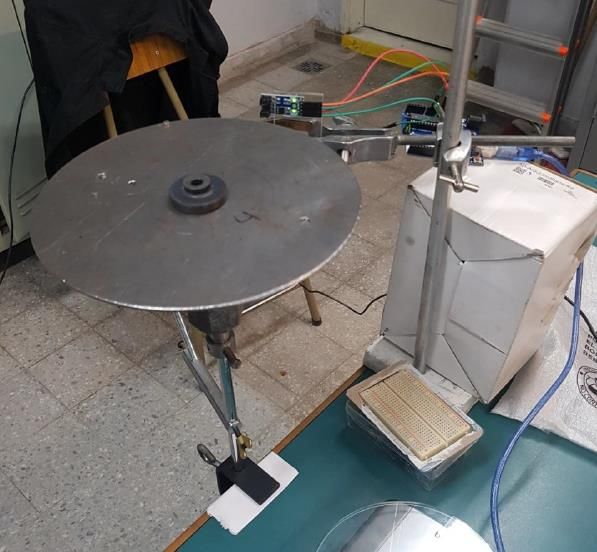
SEA-STEM 2020                                                                                                   IOP Publishing
Journal of Physics: Conference Series                         1882 (2021) 012139          doi:10.1088/1742-6596/1882/1/012139

Computational models and experimental validation at the
physics teacher training college using scilab and arduino™

                     Carlos Dibarbora1
                     1
                         National Superior Institute of Technical Teaching, Universidad Tecnológica
                         Nacional (INSPT-UTN), Av. Triunvirato 3174, CP 1427, Buenos Aires, Argentina

                     E-mail: carlos.dibarbora@inspt.utn.edu.ar

                     Abstract. This work provides an overview of the main activities developed for an Information
                     Technology course at Physics Teacher Training College - an 80 minutes per week, two semesters
                     long course in a four-year physics teachers program - which incorporates the modelling process
                     as a core topic. It proposes the implementation of software tools to aid this process, focusing
                     mainly on physics models rather than technicalities associated with the underlying math, which
                     is solved using numerical techniques. It also focuses on the experimental validation as a
                     fundamental part of the process which in this case is solved using low cost and easy accessible
                     materials as Tracker software or the Arduino boards and sensors, and describes the teaching
                     strategies implemented to reach that goal, assessed through students’ productions.

1. Introduction
The value of simulation and computational modelling in the curriculum of physics has been discussed
many times and it has been proved that the use of pre-built simulation is valuable to the learning-teaching
process [1] and that the development of the modelling process by the students has a didactic value to the
future physicists [2].
    In the education of future certified teachers, however, the graduates will teach physics in middle and
high school settings and they will work with simple deterministic models. Here, the modelling process
as a means for solving problems has real value in terms of learning, but computational modelling is a
technique not so widely researched in the field of physics education.
    In this paper, we describe the teaching strategies and tasks that we develop during an academic year
with the third year students from the physics teaching program offered in the National Technical
Teaching Institute from the Argentinian National Technological University (INSPT-UTN from its
initials in Spanish: “Instituto Nacional Superior del Profesorado Técnico - Universidad Tecnológica
Nacional”). These tasks and strategies were implemented as part of the STEM curriculum of the course
Information Technology III (Original name “Computación III”) which since 2014, has had 32 students
who have passed it.
    The program we are referring to is a course of studies to get a bachelor degree which is not the same
degree as the one held by the physicists who work in research and industries. Teacher trainees have less
math and physics credits, but they are required get some credits in education courses. Getting this degree
means national certification for teaching physics in middle and highschool and that is the main career
the graduates can pursue.
    The main goal of the course is that the students must be able to make connections between dynamical
models represented by ordinary differential equations which describe ideal situations, and the real
              Content from this work may be used under the terms of the Creative Commons Attribution 3.0 licence. Any further distribution
              of this work must maintain attribution to the author(s) and the title of the work, journal citation and DOI.
Published under licence by IOP Publishing Ltd                          1
SEA-STEM 2020                                                                               IOP Publishing
Journal of Physics: Conference Series           1882 (2021) 012139    doi:10.1088/1742-6596/1882/1/012139

physical phenomena which they have to measure using technological tools like Tracker software and
the Arduino platform with sensors, generalizing the proposals of Calderon [3], Rubinstein and Schenoni
[4], between a great variety of works and dissertations with this theme.

1.1. Theoretical framework and context
There are numerous published works about different uses of simulations in physics education, and about
how students assess learning with different approaches and theoretical frameworks [1][5][6][7].
    This course is oriented to future teachers who will use simulations in their pedagogical practices.
One of the main goals is that they learn to recognise possibilities and limitations of specific simulation
or computational models, while they gain some familiarity with the process of construction of these.
Future teachers are probably not going to develop their own simulations to teach a topic, but in this
course they will reflect about them and the important elements to be considered when using these tools.
    In Argentina, to be a physics teacher you must obtain a specific four years degree (“Profesorado”)
that is similar to a bachelor degree which you can get in some colleges. To be a physicist, on the other
hand, you must study in different colleges, and get a 5 or 6 year degree. These are by tradition, different
courses of studies with different careers and different social backgrounds. This means that people who
study to be a teacher, will only be able to use their degree to work as a teacher. There are exceptions but
this means that the curriculum is not the same for teachers as for physicists.
    The course has a duration of two semesters, with an 80-minutes lesson per week, so it is not an
important course, but it is a mandatory one.
    We can distinguish between two types of computer models in physics. These are exploratory models,
which allow students to interact with pre-built models handling their parameters to visualize different
results and behaviours, and expressive models which are the richest. The expressive models allow
students to express their own ideas on a domain, specifying relationships between concepts and different
variables and exploring the consequence of those representations. In this line of work, they learn through
an active process [5].
    In a constructivist learning environment, students do not receive the knowledge, they are not passive
listeners. Bonwell and Eison say “it is proposed that strategies promoting active learning be defined as
instructional activities involving students in doing things and thinking about what they are doing” [8].
    Students at INSPT-UTN already possess the basic physics knowledge but through the models they
build, they can go deeper into the topics and strengthen the existent relations from the explicit model.
One of the main advantages of the computational models is that they allow students to add relations and
parameters beyond the point where the math model is virtually unsolvable, or really hard to solve using
the traditional methods for differential equations, but is still within the range of numerical calculation
methods.
    The cycle for making a simulation or building a computational model has a vital step which is
‘Validation’, which is fundamental in engineering and science to guarantee the predictions of the model
will be reliable. The results obtained from the computational model must be validated comparing them
with empirical data, providing feedback to improve or change the model [9].
    One important clarification about computer models and simulations is that they do not necessarily
predict every phenomenon corresponding to a given field. There will always be a set of initial conditions
for which the model will not be able to predict valid results and there will be an uncertainty associated
with that model. For example, we could have a computer program which runs a simulation according to
Newtonian dynamics, but if the size of the objects were comparable to the size of atoms, the model
would not represent the reality.
    The modelling process proposed by Hestenes [9] constitutes not only the description of the models
construction process from an epistemological point of view but also the main topic of his ‘theory of
physics instruction’ [2] which has now been further developed but still has value for future teachers.

                                                     2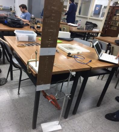
SEA-STEM 2020                                                                                 IOP Publishing
Journal of Physics: Conference Series            1882 (2021) 012139     doi:10.1088/1742-6596/1882/1/012139

                          Figure 1. Modeling process proposed by Hestenes [9]

The students are not going to be physicists or do formal science, but they are going to teach it and they
must have some scientific abilities to do that. The tasks they must perform to build a computer model,
validate it experimentally, and use the results of these comparisons to describe the limits of validity of
the model, plus the writing of a final paper describing the whole process, requires them to practice the
seven scientific abilities: A. the ability to represent physical processes in multiple ways; B. the ability
to devise and test a qualitative explanation or quantitative relationship; C. the ability to modify a
qualitative explanation or quantitative relationship; D. the ability to design an experimental
investigation; E. the ability to collect and analyze data; F. the ability to evaluate experimental predictions
and outcomes, conceptual claims, problem solutions, and models, and G. the ability to
communicate[10].

2. Methods
2.1. Implementation
During the course a lot of different activities with the computer were conducted with the goal of
providing students with the necessary Information Technology skills for developing their own computer
models, designing their own experiments with Arduino and being able to analyze and compare results.
    The software packages involved have changed with the years but the core toolkit consists in a
programming language (currently we use Scilab and Python), numerical methods to solve ordinary
differential equations [11][12] and some apps which allow us to digitize physical information such as
Tracker software, or Arduino with some sensors.
    Once students achieved sufficient competence with these tools, they were able to move forward to
the main activity, and develop their own model for a real situation, with the respective validity tests.

2.2. Simple models and numerical solutions. How to build a model?
The course standard procedure to build a dynamical mechanical model, starts by applying Newton’s
second law of motion for every element in the system. The goal is to get an expression for the

                                                       3
SEA-STEM 2020                                                                                 IOP Publishing
Journal of Physics: Conference Series           1882 (2021) 012139      doi:10.1088/1742-6596/1882/1/012139

acceleration of every particle in the system (1). Once the student has a differential equation system for
the accelerations of the particles, the remaining step is to integrate those equations to get the position
and velocity of the elements of the physical system.
    The integration of the equation system is not an ability we are trying to develop in this course, so the
students use numerical methods to get the results. Once they have built the model, they can modify the
parameters, add new parameters to analyze the qualitative behaviour of the system, or if they want
reliable numerical results, reduce the time step and improve the numerical results.

    Figure 2. Position, velocity and acceleration of Figure 3. Two bodies problem. Trajectory of
    the throwing of a spherical body considering Jupiter around the sun, solved using Euler-
    friction with the air, done by a student.        Cromer method in Scilab by another student.

The numerical method we chose to solve the differential equations is the Euler method (figure 4), for
its simplicity, and as a means to keep the focus of the task in looking for the right parametrization of the
formal model and not spending time in the implementation of more complex algorithms. Some students
have chosen to implement more advanced two and four steps algorithms, but they are allowed to do it
only once they have understood the goal of the task.

                                                          Figure 4. Euler algorithm for a particle traveling
                                                          in one dimension considering friction with a
                                                          viscous fluid as a linear term. The core of the
                                                          “simulation” has only five code lines.

2.3. Experimental measures and data acquisition
There are numerous tools for measuring and digitizing data from a physical system. In this course the
selected tool to get position values and time intervals with a camera was Tracker, and since 2017
Arduino has been incorporated into the course syllabus. The reason behind this incorporation was that
the majority of schools in Argentina where future teachers are going to work have poorly equipped labs,
and Arduino represents a cost-efficient solution to this problem, with capability for handling digital and
analog sensors for a wide range of physical variables.
    Arduino is an electronic computer that allows users to process different measurements obtained with
devices like photogates, position and temperature sensors, and it is available for a cost that goes from
five to fifteen american dollars. The students complete some simple tasks to train their programming
and electronics skills: making the connections to measure small currents and voltages directly with
analog ports (figure 5); controlling some actuators like LEDs and DC motors; and configuring some
sensors like ultrasonic position sensor HC-SR04 or photogates made with IR LED and phototransistors
(figure 6).

                                                      4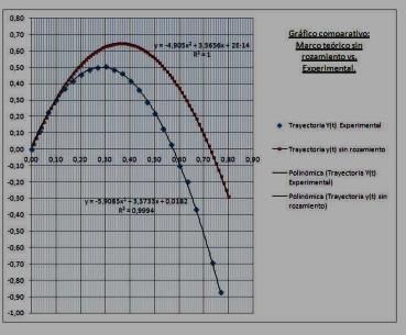
SEA-STEM 2020                                                                               IOP Publishing
Journal of Physics: Conference Series          1882 (2021) 012139     doi:10.1088/1742-6596/1882/1/012139

 Figure 5. Arduino device measuring voltages vs          Figure 6. Photogate prototype built by students
 time on a RC circuit                                    with a phototransistor and an IR LED.

3. Results and Discussion
3.1 Students’ STEM project and final papers
Students choose the physical situation they want to represent. They define their system, build a simple
model and design an experiment to measure one or more of their model’s parameters. As they make
measurements, they refine the model to adapt it to reality, and the experiment to find the limits of
validity of the model. Once they have gathered enough data, they write a final paper.
    Students have developed a variety of projects in topics such as mechanics, electromagnetism and
thermal systems. Here we present some examples of the productions highlighting their distinctive
characteristics.
    Some of the projects developed which involved Tracker to get the experimental data were flying and
falling objects - modeled taking on account air viscosity and friction-, ball collisions and pendulum.
Using Arduino, students chose to study oscillatory systems more than once, including simple and
physical pendulums (figure 7), non punctual pendulums and damped spring-mass systems. Generally
they used ultrasonic sensors to measure positions for these systems, but they also measured periods with
photogates. Regarding photogates, they studied steel flywheels twice (figure 8) and once a student
measured the speed of a little ball launched with a cannon at different heights.
    Regarding thermal systems, they used temperature sensors to model a body being heated by an
incandescent lamp, and different color bodies with hot water inside cooling down. In electromagnetism
the only projects they have developed so far are resistor-capacitor circuits.

 Figure 7. Physical pendulum. A rectangular Figure 8. A steel flywheel moment of inertia
 wood piece. The period is measured with measured indirectly with a speed sensor lm393
 homemade plastic pipe photogate, placed in which is a little integrated photogate.
 different heights.
   It is important to mention that these models and experiments are not original nor special - this is
not a requirement. They are simple experiments designed by students to acquire data about one or

                                                     5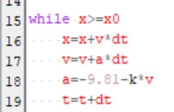
SEA-STEM 2020                                                                            IOP Publishing
Journal of Physics: Conference Series         1882 (2021) 012139   doi:10.1088/1742-6596/1882/1/012139

more variables of the mathematical model, to compare and obtain information from the physical
situation as feedback for the model.

   Figure 9. Example of a first approach to the study of a flying object, when the model without
        considering air friction is clearly divergent with the data acquired from measures.

3.2. Assessment
The way to assess the project was through examining the final papers submitted by the students. We
developed a grid with the fundamental topics that must be included in every student project to prove
that the task was satisfactorily completed (table 1). Students who had covered every topic with enough
depth in their final productions, passed the course, and students who were not able to comply with the
standard, or did not approach some topic, received personal feedback and recommendations to improve
upon their work, and reach the minimum expected level.

                                                   6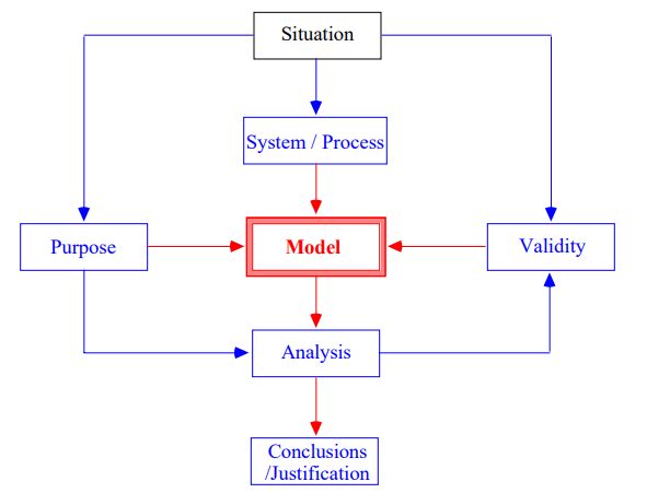
SEA-STEM 2020                                                                              IOP Publishing
Journal of Physics: Conference Series           1882 (2021) 012139   doi:10.1088/1742-6596/1882/1/012139

                            Table 1. Main indicators for assessing the task success

Fundamental points                                        Description
Relevance               Choice of a real situation that is pertinent to physics. Which allows students to
                        build a model.
Quality of analysis     This topic relates to the model, its complexity, the variables and parameters
                        identified on it and the possible representations. The model must have at least
                        one ordinary differential equation
Experiment to test      Technical validity of experiment. The design of the experiment, deciding which
validity                results are valids, sources of error, dependence between variables
Depth of analysis    This topic refers to the contrast phase. Quantity of observations and experiments,
                     thoroughness, quantity of data obtained and evaluation of the experiment vs
                     model.
Validity of computer Technical validity of the computer model. Selected algorithm, code, and initial
model                conditions. How much the model represents the chosen situation and how good
                     it is programmed.

   Since 2017, new categories were added to that list, not as minimum requirements to pass the course
but simply to give a more complete feedback to students. The added topics related to the identification
of hypotheses (explicit and implicit), the decisions taken to simplify or to put boundaries to the model,
and other sub abilities related to the experimental design, were taken from the rubrics available in [10].
   For the last few years we have been taking the feedback the students have given us into account to
modify the tasks and the assessment grid we use to evaluate them.

4. Conclusions
This is a minor course in the general structure of the physics education program, but the tasks are
significant for the future teachers as they apply real scientific abilities.
    The students take the initiative. They decide what they want to model and how they want to measure
a real system. They have to practice their experimental, mathematical, and programming skills and, if
they use Arduino to build their experiment, they practice their electronics skills too. Many STEM skills
are also put into practice. They are not going to be physicists -because in Argentina that requires a
different degree- but before graduating they will have experienced working as if they were scientists,
which is fundamental for future science teachers.
    While designing their experiments, students try out some low cost technology they can use when
teaching in the schools, which usually have low budgets for science and lab equipment. Moreover, they
learn how to think about these technologies before using them, taking into account the scope of each
sensor and tool.
    Finally, as an active learning strategy, it is engaging: students have repeatedly claimed so in their
final feedback.

References
[1] García Barneto A, Gil Martín M 2006. Entornos constructivistas de aprendizaje basados en
        simulaciones informáticas Rev. Elect. de Ens. de la Ciencia. 5 2 304-322
[2] Hestenes D 1987 Toward a modeling theory of physics instruction Am. J. Phys. 55 5 440-454
[3] Calderón S, Nuñez P, Gil S 2009 La cámara digital como instrumento de laboratorio: estudio del
        tiro oblicuo Lat. Am. J. Phys. Educ. 3 1 87–92
[4] Rubinstein J, Schenoni A 2007 Modelado de una caída de un cuerpo en aire en el laboratorio de
        física básica universitaria Rev. Argentina Enseñanza de la Ing. 8 14 57–64

                                                     7
SEA-STEM 2020 IOP Publishing
Journal of Physics: Conference Series 1882 (2021) 012139 doi:10.1088/1742-6596/1882/1/012139
[5] Jimoyiannis A, Komis V 2001 Computer simulations in physics teaching and learning: a case
study on students’ understanding of trajectory motion Comput. Educ. 36 2 183–204
[6] Holton D 2010 How People Learn with Computer Simulations Handbook of Research on Human
Performance and Instructional Technology Ed H Song and T Kidd (New York: IGI Global)
[7] Alzugaray G, Massa M, Moreira M 2014 La potencialidad de las simulaciones de campo eléctrico
desde la perspectiva de la teoría de los campos conceptuales de Vergnaud Lat. Am. J. Phys.
Educ 8 1 91-99
[8] Bonwell C, Eison J 1991 Active Learning: Creating Excitement in the Classroom. ASHE-ERIC
Higher Education Report (Washington DC: George Washington University)
[9] Hestenes D 1996 Modeling Software for learning and doing physics Thinking Physics for
Teaching Ed C. Bernardini et al (New York: Plenum)
[10] Etkina E, Van Heuvelen A, White-Brahmia S, Brookes D, Gentile M, Murthy S, Rosengrant D,
Warren A 2006 Scientific abilities and their assessment Phys. Rev. ST Phys. Educ. Res. 2
020103
8You can also read