Explore and Control with Adversarial Surprise - arXiv
←
→
Page content transcription
If your browser does not render page correctly, please read the page content below

Explore and Control with Adversarial Surprise

                                                      Arnaud Fickinger∗1 , Natasha Jaques∗12 , Samyak Parajuli1 , Michael Chang1 ,
                                                         Nicholas Rhinehart1 , Glen Berseth1 , Stuart Russell1 , Sergey Levine12
                                                                                     1
                                                                                       UC Berkeley
                                                                             2
                                                                               Google Research, Brain Team
                                                         arnaud.fickinger@berkeley.edu, natashajaques@google.com
arXiv:2107.07394v1 [cs.LG] 12 Jul 2021

                                                                                          Abstract

                                                      Reinforcement learning (RL) provides a framework for learning goal-directed
                                                      policies given user-specified rewards. However, since designing rewards often
                                                      requires substantial engineering effort, we are interested in the problem of learning
                                                      without rewards, where agents must discover useful behaviors in the absence
                                                      of task-specific incentives. Intrinsic motivation is a family of unsupervised RL
                                                      techniques which develop general objectives for an RL agent to optimize that lead
                                                      to better exploration or the discovery of skills. In this paper, we propose a new
                                                      unsupervised RL technique based on an adversarial game which pits two policies
                                                      against each other to compete over the amount of surprise an RL agent experiences.
                                                      The policies each take turns controlling the agent. The Explore policy maximizes
                                                      entropy, putting the agent into surprising or unfamiliar situations. Then, the Control
                                                      policy takes over and seeks to recover from those situations by minimizing entropy.
                                                      The game harnesses the power of multi-agent competition to drive the agent to
                                                      seek out increasingly surprising parts of the environment while learning to gain
                                                      mastery over them. We show empirically that our method leads to the emergence
                                                      of complex skills by exhibiting clear phase transitions. Furthermore, we show both
                                                      theoretically –via a latent state space coverage argument– and empirically that our
                                                      method has the potential to be applied to the exploration of stochastic, partially-
                                                      observed environments. We show that Adversarial Surprise learns more complex
                                                      behaviors, and explores more effectively than competitive baselines, outperforming
                                                      intrinsic motivation methods based on active inference, novelty-seeking (Random
                                                      Network Distillation (RND)), and multi-agent unsupervised RL (Asymmetric Self-
                                                      Play (ASP)) in MiniGrid, Atari and VizDoom environments.

                                         1       Introduction
                                         Despite promising results across a number of domains (e.g., [5, 26, 28, 46]), a major challenge in
                                         reinforcement learning (RL) is that the effectiveness of current methods depends heavily on task-
                                         specific rewards [34, 45]. For many tasks, designing dense and informative rewards require significant
                                         engineering effort, and sparse rewards make learning slow and difficult [34, 45]. Yet humans and
                                         animals easily learn from their own experience without being constantly told what to do. Therefore,
                                         significant prior research has focused on developing a class of unsupervised RL methods that optimize
                                         for intrinsic motivation (IM) – alternative objectives (such as seeking novelty) that incentivize the
                                         agent to autonomously explore and learn about the world without being entirely dependent on explicit
                                         goals and task incentives.
                                         Many prior works have approached the problem of unsupervised RL as one of pure novelty-seeking,
                                         training agents to optimize for surprise in the hopes of facilitating better exploration, which can
                                             ∗
                                                 Equal contribution.

                                         Preprint. Under review.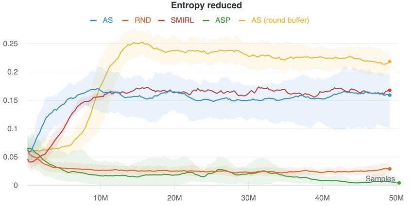
(a) Adversarial game                     (b) Explore and Control policy taking turns

Figure 1: Adversarial Surprise is a multi-agent competition in which two policies take turns controlling
an RL agent. The Explore policy acts first, and tries to put the agent into surprising, high entropy
states. On its turn, the Control policy tries to minimize surprise by finding familiar, low-entropy,
predictable states. Figure (b) shows an example rollout of a game. In the Explore policy’s first turn, it
attempts to maximize entropy by remaining in the first room with flashing lights (a noisy TV state).
When the Control policy takes over, it is able to take an action to control the environment, by flipping
the switch to stop the lights from flashing. Therefore, when the Explore policy acts again it moves
into the next room; this is predicted by our theoretical results, which show that the Explore policy
must maximize entropy over the true state space. During the Control policy’s next turn it remains in
the dark room. This process continues until all of the rooms have been visited.

be helpful for learning downstream tasks. However, current novelty-seeking methods don’t always
produce the desired explorative behavior. In stochastic environments for example, such methods can
suffer from the “noisy TV" problem where the agent becomes distracted by inherently high-entropy
elements [39]. In contrast, some biologically-inspired approaches like active inference suggest
that complex human-like behaviors are obtained by minimizing the expected surprise on future
observations [15, 18, 6]. However, in the absence of an informative observation prior that guide the
agent towards interesting behaviors, such methods suffer from the “dark room" problem [16]: if what
the agent can observe from the environment is not surprising, the agent will not be incentivized to
learn any complex behavior. This is especially problematic in partially-observed environments. Yet
humans seem to always maintain a tension between optimizing for both novelty and familiarity. For
example, a child in a play room does not just try to toss their toys on the floor in every possible
pattern, but instead tries to stack them together, find new uses for parts, or combine them in various
ways. In the same way, we suggest that the right objective for unsupervised RL should be to actively
maintaining a tension between exploration and control. Such method would have the potential to
produce increasingly complex and interesting behaviors without the limitations of optimizing for
novelty or familiarity alone.
In this paper, we maintain a tension between exploration and control by formulating an adversarial
game between two policies, which each take turns sequentially acting for the same RL agent. The
Explore policy is novelty-seeking, and attempts to maximize surprise over the course of the episode,
putting the agent into a diverse range of novel states. In turn, the Control policy must minimize
surprise, by learning to manipulate its environment in order to return to safe and predictable states.
When combined, the two adversaries engage in an arms race, repeatedly putting the agent into
challenging new situations, then attempting to gain control of those situations. Figure 1 shows an
illustration of the method, including a sample interaction. Rather than simply adding noise to the
environment, the Explore policy learns to adapt to the Control policy, and to search for increasingly
challenging situations from which the Control policy must recover. Thus our method, Adversarial
Surprise (AS), leverages the power of multi-agent training to generate a curriculum of increasingly
challenging exploration and control problems. We show empirically that the competition between
the two policies produces the emergence of increasingly complex observable behaviors in the agent
by exhibiting clear phase transitions. Furthermore, we show theoretically and empirically that the
increasingly complex control and exploration strategies found by the competing policies enable
the efficient exploration of stochastic, partially-observable environments that previous methods
optimising for novelty or familiarity alone fail to explore.
Our main contribution is the Adversarial Surprise (AS) algorithm, an unsupervised RL method
to actively maintain a tension between exploration and control which leads to the emergence of
increasingly complex behaviors. We derive our method, and perform a theoretical analysis in the
recently introduced Block MDP setting [12] which shows –via a latent space coverage argument–

                                                   2
that our method can be applied to the exploration of partially-observed, stochastic environments.
We present a practical instantiation based on deep reinforcement learning, and provide an empirical
evaluation that compares our approach to recent intrinsic motivation and unsupervised RL techniques.
Our results demonstrate that our method induces the emergence of complex behaviors that can be
used for both control and exploration. As suggested by our theoretical results, we show empirically
that our method can be applied to the exploration of partially-observable, stochastic environments,
outperforming previous methods like Random Network Distillation (RND) [7], Suprise-Minimization
RL (SMiRL) [6] and Asymmetric Self Play (ASP). We also show that AS produces more meaningful
behaviors in VizDoom [24] and Atari [3] without any external reward.

2   Related Work

Our method enables the emergence of complex skills without supervision and thus enters into the
budding field of unsupervised RL that we briefly survey below. A common strategy in this field is to
formulate a task-agnostic objective that uses environment statistics only and to derive an intrinsic
reward that enables exact or approximate optimization of this objective using standard RL algorithms.
A recurrent question in this field is the applicability of the skills learned. We will show that our method
has the potential to be applied to the exploration of stochastic, partially-observable environments.
Novelty-seeking intrinsic motivation: One of the most frequently studied forms of intrinsic motiva-
tion is novelty-seeking, or curiosity, which can be formulated as maximizing the information gain on
the agent’s dynamics model of the environment [20, 42, 4, 32, 37]. Common intrinsic rewards used
to approximate curiosity include surprise [1, 37, 48, 32, 7] and ensemble disagreement [41, 33]. A
novelty-seeking agent is motivated to explore its environment. However, naïvely maximizing surprise
leads to methods that are vulnerable to the noisy TV problem, where the agent becomes distracted by
inherently high-entropy, unpredictable elements in the environment, such as white noise (e.g. static
on a TV) [39]. In this case, a curious agent will not be able to learn meaningful behaviours. We will
show that AS overcomes this problem, and fully explores the state space even when there are highly
stochastic elements.
Surprise minimization and the free energy principle: Rather than maximizing surprise, the free
energy principle [13, 15, 18, 17, 44] proposes that biological agents actually minimize long-term
average surprise by seeking familiar, stable states, and controlling their environment to make it more
predictable. Inspired by this idea, Berseth et al. [6] built a surprise-minimizing RL agent, SMiRL,
which outperforms curiosity-maximizing methods like ICM [32] in high-entropy environments.
However, in partially observed or low-entropy environments, surprise minimization is vulnerable to
the dark room problem: if the agent can simply stay in a highly-predictable part of the environment
where nothing happens, it will [16]. In this scenario, a surprise-minimizing agent cannot learn
meaningful behaviors either. AS is designed to avoid this problem, because the Explore policy will
not allow the Control policy to remain in a dark room.
Empowerment: The goal of empowerment [25, 36] is to maximize the mutual information between
the agent’s actions and its future states. Empowerment encourages agents to “keep their options open"
by exploring many states, while still maintaining a high degree of control in those states. However,
calculating empowerment in high dimensional environments is intractable, leading to various methods
for approximating it (e.g., [22, 35, 50, 9, 49, 21, 30]). Unfortunately, these methods can also be
difficult to get working with high dimensional function approximation [19]. In contrast, we show that
Adversarial Surprise works with deep neural networks applied to pixel inputs in Atari environments.
Emergence in multi-agent setting: Multi-agent competition can provide a mechanism for driving
RL agents to automatically learn increasingly complex behavior [27]. As each agent adapts, it
makes the learning problem for the other agent increasingly difficult, leading to the emergence of an
automatic curriculum of challenging learning tasks [2, 10, 47, 14]. For example, Schmidhuber [38]
proposed having two classifiers compete by repeatedly selecting examples which they can classify
but which the other cannot. Asymmetric Self Play (ASP) [43, 31] rewards one agent, Alice, for
executing the shortest trajectory that a second agent, Bob, cannot copy (or reverse). Similarly to ASP,
Adversarial Surprise is formulated as an adversarial game between two policies. However, unlike
ASP our method is formulated in terms of general information theoretic quantities which make it more
generally applicable. For example, we show that ASP can fail to explore stochastic environments,

                                                    3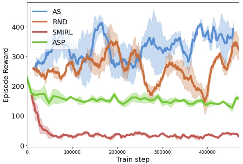
because Alice can easily produce a random goal state which Bob is not able to reproduce. In contrast,
AS works well in stochastic environments, outperforming ASP.

3   Background
Partially Observed Markov Decision Process: A POMDP is a tuple (S, A, T , O, r, γ), where
s ∈ S are states, a ∈ A are actions, r(a, s) is the reward function, and γ ∈ [0, 1) is a discount
factor. The environment is partially observed, so the agent cannot observe the true state s, but rather
observes o ∼ p(O|s). At each timestep t, the agent selects an action at according to its policy
π(at |ot ), receives reward r(at , st ), and the environment transitions to the next state according to
T (st+1 |st , at ). We are interested in stochastic environments, in which the emission distribution
distribution is inherently entropic for some states, i.e. ∃s : H(p(O|s)) > 0.
Block Markov Decision Process: A BMDP [12] is a POMDP with an additional disjointness
assumption: for any s, s0 ∈ S, s 6= s0 ⇒ supp(p(O|s)) ∩ supp(p(O|s)) = ∅. Our theoretical results
show that the AS algorithm fully covers the latent state space of a large family of BMDPs.
Intrinsic motivation: IM can either be used in combination with a task objective, in which case
intrinsic motivation serves to facilitate exploration, or by itself, in which case the agent receives no
external task rewards, and aims only to maximise its intrinsic objective, leading it to learn skills
that may potentially be useful for downstream tasks. In this paper, we study how an agent can learn
skilled behaviour without rewards. Therefore, we consider agents that seek to optimize cumulative
                                          PT
intrinsic reward over the episode: R = t=0 γ t ri (at , st ).
Surprise minimizing agents (SMiRL): The free energy principle [13, 15, 18, 17, 44] suggests that
biological agents may minimize surprise, or state entropy, in order to remain in safe and stable states.
Minimising surprise for an RL agent can be done by keeping track of the state history of the agent via
a density model, pθ (s), which bounds the state marginal density of the policy, dπ , given states seen
so far in an episode, τt = {s0 , ...st }. Indeed, Berseth et al. [6] shows that we can use the intrinsic
reward ri (st ) = log pθ (s) to minimize the entropy of the state marginal distribution H(dπ (s)):
                                                                   "∞                 #
                                                                    X
                        π                                                t
                   H(d (s)) ≤ −Es∼dπ (s) (log pθ (s)) = −Eπ             γ log pθ (st )               (1)
                                                                     t=0

where the bound becomes tight as log pθ (s) → dπ (st ); that is, as the density model approaches the
true state marginal density. A SMiRL agent trained with this objective learns emergent behaviors to
reduce entropy in stochastic environments—such as stable walking robots or playing Tetris—even in
the absence of any external reward. However, when applied to partially observed environments, the
agent is susceptible to the dark room problem; rather than learning to control the environment, it can
simply control its observations by remaining in unsurprising parts of the environment. Or, simply
turning to look at a wall. In our method, we build on surprise minimization, incorporating it into a
two player game that alleviates this shortcoming.

4   Adversarial Surprise
The goal of Adversarial Surprise (AS) is to produce complex behaviors that can be used for exploration
and control. To this end, AS pits two policies against each other in a two-player competition over
the amount of surprise an RL agent experiences. Specifically, we learn an Explore policy, π E , and a
Control policy, π C . The goal of the Control policy is to minimize its own surprise, or observation
entropy, using a learned model pθ (o). However, the Explore policy’s goal is to maximize the surprise
that the Control policy experiences.
The policies take turns taking actions for the agent, switching back and forth throughout the episode.
The policy controlling the RL agent change every k steps, such that:
                                E
                                   π (at |ot ) if ∃n, t ∈ [2nk, (2n + 1)k[
                          at ∼                                                                     (2)
                                   π C (at |ot ) otherwise
Each policy is given several steps to act because it enables it to reach states that will be challenging for
the other policy to recover from, thus facilitating learning more complex and long-term exploration
and control behaviors (see Figure 1).

                                                     4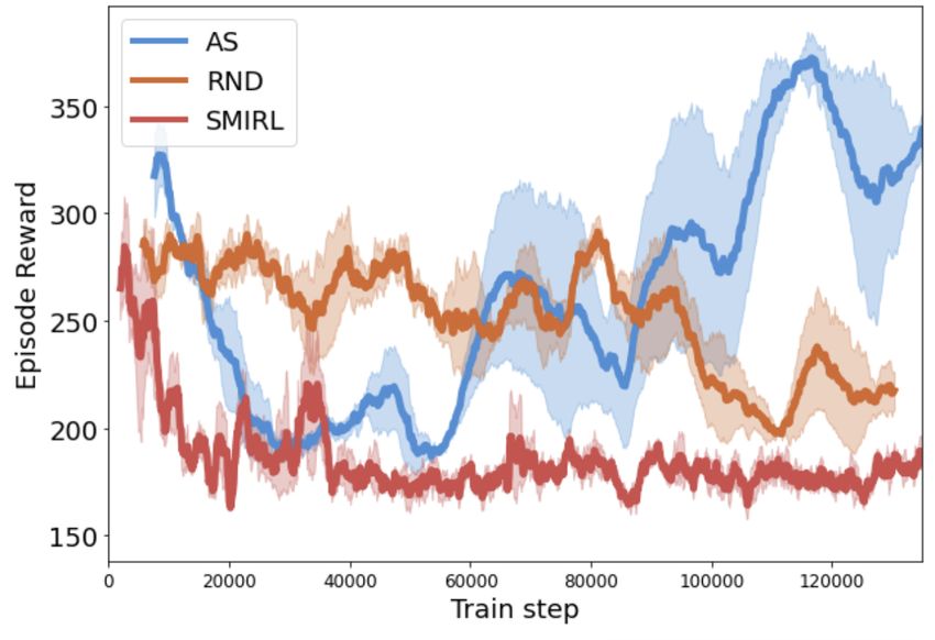
Algorithm 1: Adversarial Surprise
Randomly initialize φE and φC ;
for episode = 0, ..., M do
Initialize θ, Ri = 0, β ← {}, explore_turn = True, tC = k, s0 ∼ p(s0 ), o0 ∼ p(O0 |s0 );
for t ← 0 to T do
if explore_turn then
at ∼ π E (ot , hE
t ); // Explore
else
at ∼ π C (ot , hC
t ); // Control
end
st+1 ∼ T (st+1 |st , at ), ot+1 ∼ p(Ot+1 |st+1 ) ; // Environment step
rti = log pθ (ot+1 ) ; // Compute intrinsic reward
if not explore_turn and t − tC > k/2 then
Ri = Ri + r i ;
end
β = β ∪ {ot , at , ot+1 } ; // Update buffer
if t == tC then
explore_turn = not explore_turn ; // Switch turns
tC = tC + 2k;
end
θt+1 =MLE_update(β, θt ) ; // Fit density model
end
φE =RL_update(β, −Ri ) ; // Train Explore policy π E with reward −Ri
C i
φ =RL_update(β, R ) ; // Train Control policy π C with reward Ri
end
To estimate surprise, we learn a density model which estimates the agent’s likelihood of experiencing
observation o, pθ (o). Because the Control policy is surprise-minimizing, its reward is riC (st ) =
log pθ (ot ), which resembles SMiRL [6], except using the observation in place of the state. The goal
of the Explore policy is to maximize the observation surprise of the RL agent when the Control policy
is in control. This creates an adversarial game, in which the Explore policy attempts to find surprising
situations with which to expose the Control policy, and the Control policy’s objective is to recover
from them. Therefore, the Explore policy’s reward is based on the surprise for the observations of the
Control policy. Assume that the Control policy’s turn begins at timestep tC , and it receives a total
PtC +k
reward of Ri = t=tC γ k ri (at , st ) for that turn. Then, the Explore policy’s reward is −Ri , and
is applied to the last timestep of the Explore policy’s turn (i.e. timestep tC − 1). The full training
procedure for Adversarial Surprise is given in Algorithm 1.
Thus, Adversarial Surprise defines the following adversarial game between the two policies:
C
tX+k
max min −E log pθ (ot ) , (3)
πE πC
t=tC
where the Explore policy can only effect p(ot ) through the final state that it produces at the end
of its turn, which is the initial state for the Control policy. We show in Appendix Section A the
equivalent of eq. 1 in the partially observable setting. As a corrolary, the objective of the Explore
policy approaches maximizing the entropy of the Control policy’s observations:
C
tX+k
J E = −E log pθ (ot ) ≈ H(dπC (o)), (4)
t=tC
Analogously, the Control policy’s goal is to minimize entropy:
C
tX +k
JC = E log pθ (ot ) ≈ −H(dπC (o)) (5)
t=tC
5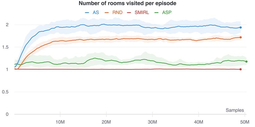
Implementation details: We parameterize the policies for the Explore and Control policy using
deep neural networks (NN) with parameters φE and φC , respectively. We policy is based on a
convolutional NN which conditions on a stack the last 4 observation frames. The networks are trained
using Proximal Policy Optimization (PPO) [40]; further details and hyperparameters are given in
Appendix B. Following [6], the density model pθ (o) is re-initialized each episode and trained using
maximum likelihood estimation (MLE) to fit the observations of the agent within a single episode,
which are stored in a buffer β. The density model is either represented using a Gaussian distribution
as in [6], or using independent categorical distributions. We have found it helpful to only compute
the surprise reward using observations from the second half of the Control policy’s turn; this gives
the agent greater ability to take actions that may lead to initial surprise, but reduce entropy over the
long term. We also experiment with when to reset the buffer β; we find that resetting the buffer after
each round (after the Explore policy and Control policy each take one turn) can sometimes improve
performance. Finally, we allow the Explore and Control policys to act for a different number of
timesteps, tuning the emphasis on exploration or control depending on the environment.

5   Adversarial Surprise maximizes state coverage in Block MDPs
In this section, we show that our method covers the state space under some restrictions on the
structure of the POMDP, and the density of states with low observation entropy. Full proofs are in the
Appendix.
                                                                          P∞
We define the marginal observation distribution as: dπ (o) = (1 − γ) t=0 γ t p(ot = o). We are
interested in maximizing the state marginal entropy dπ (s) by using a density model of the observation,
pθ (o). To that end, we prove the following lemma in Appendix Section A:
Lemma 1. The cumulative surprise measured by the observation density model pθ (o) forms an upper
bound of the observation marginal entropy H(dπ (o)), which P∞ becomes tight when the observation
density model fits the observation marginal dπ (o): −Eπ t=0 log pθ (ot ) ≥ H(dπ (o))

We start with an assumption on the structure of the POMDP:
Assumption 1 (Block MDP (BMDP) [29]). We suppose that every two different states have disjoint
emission supports: for any s, s0 ∈ S, s 6= s0 ⇒ supp(p(O|s)) ∩ supp(p(O|s)) = ∅

Under this assumption, we show a useful relation between observation marginal entropy and state
marginal entropy:
Lemma 2. In a BMDP, we can decompose the observation marginal entropy:
                          H(dπ (o)) = Edπ (s) H(p(O|S = s)) + H(dπ (s))                             (6)

See Appendix Section A for the proof. Equation 6 shows that maximizing entropy in the marginal
observation distribution dπ (o) amounts to maximizing two terms: the emission entropy H(p(O|S)),
and the state marginal entropy H(dπ (s)).
Suppose that we have a small number of latent states with rich observations, i.e. where the entropy of
the emission distribution is very high: ∃s : H(p(O|S = s))  log |S|. We can think of these states
as “noisy TVs". In this case, if we are trying to maximize the marginal observation entropy, we have:
                           max H(dπ (o)) ≈ max Edπ (s) H(p(O|S = s))                                (7)
                           dπ (s)          π  d (s)

The RHS is maximized by taking:
                             dπ (s) = 1(s = arg max H(p(O|S = s)))                                  (8)
                                                 s∈S

This shows that conventional methods that focus on maximizing entropy over observations can
trivially maximize dπ (o) by remaining in a state with rich observation. We will show that Adversarial
Surprise is not subject to this problem.
To this end, we define a (semiquasi)metric on the latent state space: d(s,       ˜ s0 ) = min{k :
       π 0                                        π
∃π, Pk (s |s) = 1}, where by convention P0 (s|s) = 1 for all s. In other words, d(s,      ˜ s0 ) = k
if there is a policy that reaches s0 from s in k steps with probability 1. We symmetrize this metric by
defining the following semimetric: d(s, s0 ) = max{d(s, ˜ s0 ), d(s
                                                                 ˜ 0 , s)}

                                                   6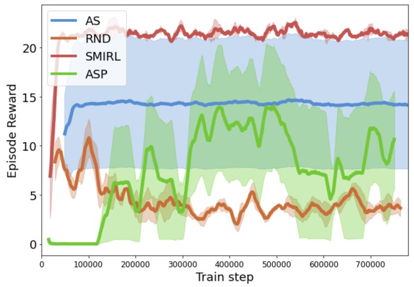
We now give a formal definition of dark rooms. We say that a state s is a dark room if it has
minimal emission entropy: H(p(O|S = s)) = mins∈S H(p(O|S = s)). We will use the following
assumption about the density of dark rooms in the latent state space:
Assumption 2. We make three assumptions concerning the density of dark rooms:

     (a) We suppose that for every state s, there is a dark room such that d(s, s0 ) ≤ T . That is, the
         set of dark rooms is a T -cover of the state space with respect to d.
     (b) We suppose that for every state s, there is a dark room such that PTπ (s0 |s) = 1, that is a
         dark room can be reached in exactly T steps.
                                                                    ˜ s0 ) ≤ T , then d(s, s0 ) ≤ T ,
     (c) We suppose that for any state s and any dark room s0 , if d(s,
         that is if we can reach a dark room from a state s in less than T steps, then we can also
         reach s from this dark room is less than T steps.

We can now state our main result:
Theorem 1. Under Assumptions 1 and 2 the Markov chain induced by the following AS game:
                                         max        min         H (dπTC (o))                                 (9)
                                       dπE (s0 ) dπ C
                                                  1:T (s|s0 )

T -covers the state space, i.e., for all states s, there is a state s0 such that dπ (s0 ) > 0 and d(s, s0 ) ≤ T ,
where dπ is the state marginal distribution induced by the game between the Explore (πE ) and
Control (πC ) policies.

Assumption 2 guarantees that for any states that the Explore policy reaches, the Control policy can
find a low-emission-entropy state within its turn, such that H(p(O|s)) is minimized. Thus, from
the perspective of the Explore policy, the first term in its objective in Eq. 6 is minimized, and it
must focus on maximizing the second term, H(dπ (s)). In order to maximize entropy over the state
marginal distribution dπ (s), the Explore policy must fully explore the state space.

6    Experimental results
In this section we present experimental results designed to answer the following four questions:

      1. Exploration and state coverage: how well does AS explore the underlying state space
         in a stochastic, partially-observed world, as compared to alternative methods? Given our
         theoretical results in Section 5, we hypothesize that methods based on novelty-seeking will
         become distracted by noisy elements, while AS will fully explore the environment. We will
         use the number of rooms visited in a navigation task as a measurement of state coverage.
      2. Control: will AS learn to take actions to control its environment, and recover from surprising
         situations? We measure control as the number of actions taken that cause changes to elements
         in the environment, such as flipping a switch to stop flashing lights.
      3. Emergence of complexity: is AS able to produce an arms race between the Control and
         Explore policies that leads to the agent’s acquisition of increasingly complex observable
         behaviors? If this is the case, we expect to observe the alternation of relatively long learning
         phases, where the two policies are competing without visible change in the agent’s behavior,
         and relatively short phase transition that separate two clearly distinguishable behavior.
      4. No-reward learning: will AS enable the agent to learn meaningful behaviors in the absence
         of any external reward? To assess this, we train the IM methods using only intrinsic reward,
         then assess the amount of task reward they obtain in the standard Atari benchmark [3].
         While there is no reason to expect AS to always correlate with the objectives in arbitrary
         MDPs, we expect that the twin goals of maximizing coverage while achieving high control
         should correlate well with objectives in many reasonable MDPs, particularly video games
         of the sort present in Atari. Many of these games have a notion of progress, which roughly
         corresponds to coverage, but at the same time have many dangerous states that could result
         in ‘death’, which leads to an unexpected jump back to the starting state. Therefore, we
         hypothesize that AS should, without even being aware of the task reward, perform well in
         these environments. Comparing to prior methods in these domains is interesting, because

                                                         7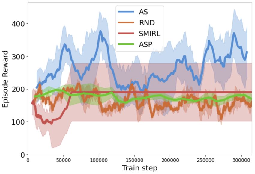
(a) Cumulative exploration                       (b) Exploration within an episode
Figure 2: Q1. Exploration and state coverage: the number of rooms explored in partially-observed
environments containing both stochastic elements and dark rooms, both (a) cumulatively over training,
and (b) within an episode. Part (a) shows how well each method works as an exploration bonus to
encourage collecting experience from all states, and part (b) provides a measure of how well the
asymptotic policy learned by each method continues to explore the state space at convergence. AS
outperforms surprise-minimizing SMiRL, which minimizes observation surprise by turning to face
the wall, or remains in dark rooms. AS also explores better than the state-of-the-art exploration
methods RND and ASP, which both become distracted by noisy elements.

         prior work has variously argued that both novelty-seeking exploration methods [7] and
         surprise-minimization methods [6] should be expected to achieve high scores in these
         domains. Note that when we assess all three metrics we look at the performance of the agent
         as a whole, which is jointly controlled by both the Explore and Control policy.

We include videos of the AS agent learning to play games with no reward, as well as performing
navigation tasks, at https://sites.google.com/view/adversarial-surprise/home.
Baselines: We compare AS to three competitive unsupervised RL baselines: Asymmetric Self-Play
(ASP) [43] (a state-of-the-art multi-agent curriculum method), Random Network Distillation (RND)
[7] (a state-of-the-art exploration method), and SMiRL [6] (a recently proposed method based on
surprise minimization). These three methods are all related to AS: like RND, the Explore policy
aims to maximize surprise, though not instantaneously but rather over the Control policy’s episode;
like SMiRL, the Control policy aims to minimize surprise, but starting from the initial states that
the Explore policy puts it in, and in a partially observed setting; like asymmetric self-play (ASP),
AS consists of a two-player game, though the AS two-player game is symmetric and zero-sum, and
based on observational entropy rather than goal-reaching. All methods use PPO as RL optimization
algorithm, with hyperparameters given in Appendix B.
Environments: To evaluate Q1 and Q2, we need partially-observed environments that present an
exploration challenge, and which include stochastic phenomena. Since standard benchmarks do
not consistently exhibit these properties, we constructed a custom family of procedurally generated
navigation tasks based on Minigrid [8]. These environments contain rooms that are either empty
(dark), or contain stochastic elements such as flashing lights that randomly change color. They also
contain elements such as doors that can be opened, and switches that, when flipped, stop the stochastic
elements from changing. An example is shown in Figure 1. As in MiniGrid, the environments are
partially observed; the agent only sees a 5x5 window of the true state. To evaluate Q3, we choose
a relatively simpler version of our custom Minigrid environment that includes only two rooms to
clearly distinguish the gain of complexity due to AS from the complexity of the environment. While
these environments allow us to carefully study the effects of partial observability and stochasticity, we
would also like to compare to prior work on a standardized benchmark. For this purpose, to evaluate
Q4 we use the Atari Arcade Learning Environment (ALE) [3] (see Figure 5), which was used by
both SMiRL [6] and RND [7] to establish their effectiveness, as well as the ViZDoom environment
[24]. Due to limited computational resources, we do not conduct experiments in all possible Atari
games (which is consistent with prior work [6, 7]), but we show results for each of the games that we
test, both in Section 6.4 and Appendix B.4.

                                                   8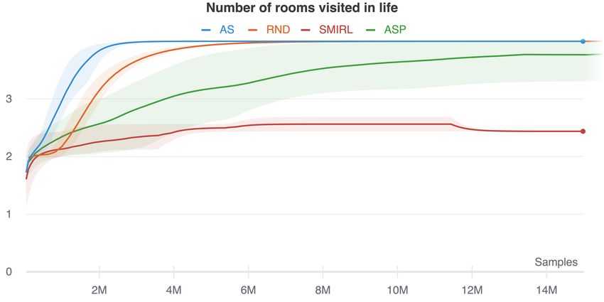
6.1   Exploration and state coverage:

Figure 2 shows the results of training the AS agent in the procedurally-generated navigation envi-
ronments in terms of the number of rooms the agent learns to visit (our measure of state coverage).
We measure the number of rooms cumulatively, over the course of training (Figure 2a), to assess
whether each method will lead the agent to collect experience from all possible states. This measure
is relevant to whether the technique can be used as an effective exploration bonus to aid learning
a downstream task. We also measure the number of rooms explored within each episode (Figure
2b). This allows us to assess whether the asymptotic policy learned by the algorithms continues to
explore once it has converged. As predicted by our theoretical analysis, we see that AS learns to more
fully explore the environments, visiting significantly more rooms over a lifetime (Figure 2a) and per
episode (Figure 2b) than competing methods. It learns more quickly and explores more thoroughly
than RND, which becomes distracted by the inherently random elements in the environment which
lead to high prediction error. The stochastic elements also hinder learning for ASP, since Alice can
easily produce random goals that are difficult for Bob to replicate. Finally, we see that SMiRL, which
is designed for fully observed environments, does not explore effectively because it suffers from the
dark room problem – it prefers to stay within the empty rooms, and not venture into rooms with
high-entropy, stochastic elements.

6.2   Control:

                                                       To measure whether the agent learn to control
                                                       their environment, we investigate how many
                                                       times the agent press switches in the navigation
                                                       environment that stop the stochastic elements
                                                       in the environment from changing color. The
                                                       results are shown in Figure 3. Since RND has no
                                                       incentive to learn to control the environment, it
                                                       never learns to press the switch. A similar result
                                                       is observed for ASP, since reducing the entropy
                                                       would make it easier for the Bob agent to repli-
                                                       cate the Alice agent’s final state. Thus, ASP will
Figure 3: Q2. Control: the average number of not always lead the agent to learn all possible be-
times the agent flip a switch to stop lights from haviors relevant to controlling the environment.
flashing. ASP and RND do not learn to press the Both SMiRL and AS learn to take actions to
switch, while SMiRL and AS both press the switch reduce entropy. However, when we train AS
a similar number of times. Resetting the AS buffer by resetting the buffer β used to fit the density
more frequently enables it to exceed even SMiRL model p (o) after each round (that is, after both
                                                                θ
in taking actions to control the environment.          the Explore and Control policy have taken one
                                                       turn), rather than after each episode, we see that
AS increases the number of actions it takes to reduce entropy even over SMiRL. This is likely because
resetting the buffer removes any incentive to return to states that the agent has previously seen within
its lifetime, and instead gives a stronger incentive to reduce entropy immediately.

6.3   Emergence of Complexity:

To show that Adversarial Surprise leads to emergence of complexity by phases, we plot the temporal
acquisition of two behaviors in order of complexity in the MiniGrid environment. The results are
shown in Figure 4. This environment includes a dark room and a noisy room separated by a door.
The position of the door changes at each episode. Initially, the agent is inside the noisy room and
the door is open. One episode consists of 96 steps: the Control policy takes control of the agent
during 32 steps, then the Explore policy takes control of the agent during 32 steps, finally the Control
policy takes control of the agent during 32 steps. The first acquired behavior by the Control policy
is identifying where the door is and going to the dark room during the first round. It is a short-
term suprise minimizing behavior and an agent trained with a SMIRL objective can converge to it.
However, the Explore policy learns to go back to the noisy room and to reach the farthest point from
the door such that the Control policy does not have the time to reach a state of minimum entropy
before the surprise of the agent is computed in the reward. This in turn incentivizes the acquisition
of a more complex behavior by the Control policy: it learns to go in the dark room and to lock the

                                                   9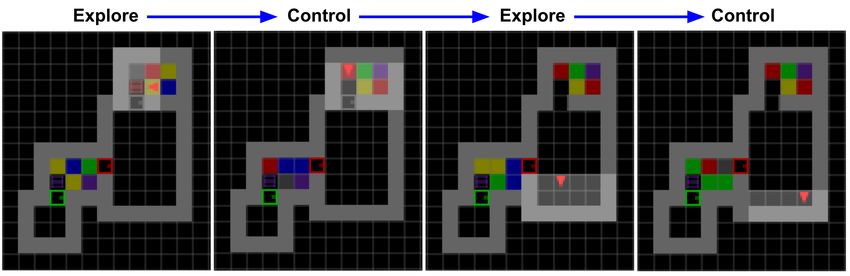
(a) Acquisition of two behaviors by phases in order of (b) The Control policy learns to lock the agent in the
 complexity and long-term impact on the surprise        dark room to minimize long-term surprise
Figure 4: Q3. Emergence of Complexity: In spite of the relative simplicity of the environment
(right), we observe two relatively short phase transitions separating three learning phases with three
clearly distinguishable behaviors: randomly exploring, going to the dark room, locking the agent
in the dark room (left). This is evidence of an emergent curriculum induced by the multi-agent
competition.

       (a) Berzerk                 (b) Assault                 (c) Freeway              (d) Space Invaders

Figure 5: Q4. No-reward learning in Atari: Each method is trained in Atari using only intrinsic
reward. Plots show how much of the true game reward the agent obtains, with error bars showing
95% Confidence Interval (CI) of three seeds. Since the games reward behavior such as staying alive
and learning to shoot enemies, obtaining higher reward indicates the agent has learned meaningful
behaviors. AS outperforms both RND and SMiRL, showing that AS provides a general way to learn
useful behaviors across multiple environments, in the absence of external reward.

agent inside by closing the door during the first round, making it harder for the Explore policy to
learn to reach a state that will surprise the agent during the Control policy’s second round. This
behavior reminiscent of Dr. Jekyll and Mr. Hyde highlights the potential of Adversarial Surprise to
learn long-term suprise-minimizing behaviors.

6.4   No-reward learning:

Figures 5 and 6 show how well each method can be used
to learn interesting behaviors in the absence of external
reward. To assess whether they can learn useful skills,
we measure the game reward obtained in several Atari
environments and the VizDoom Take Cover environment.
Because the games reward complex behaviors like shoot-
ing or avoiding enemies, a high game reward indicates the
agent has learned interesting skills, purely from optimiz-
ing the instrinsic objective. Across the environments, AS
performs better than RND, SMiRL, and ASP. While RND
is effective in some environments, its performance often
                                                                  Figure 6: Q4. No-reward learning in
decreases over time due the bonus from the prediction
                                                                  Doom. Consistent with the Atari results,
error shrinking as more states become familiar. Further,
                                                                  AS learns more meaningful behaviors
maximizing novelty in environments like Freeway, Space
                                                                  (i.e. moving while avoiding enemy bul-
Invaders, and Doom can lead to the agent dying, corre-
                                                                  lets) than other techniques. This leads to
sponding to low reward. SMiRL performs well in Freeway,
                                                                  higher environment reward during evalu-
where minimizing entropy corresponds closely to staying
                                                                  ation.
alive and not being hit by cars. However in the other en-
vironments, SMiRL performs poorly, because it avoids

                                                      10
entropy by hiding from enemies (it prefers to stay in dark rooms when they are available). ASP also
performs poorly because it is possible for Alice to quickly reach states which Bob cannot easily
replicate, preventing the algorithm from learning meaningful behaviors. In contrast, AS consistently
obtains high returns across all environments, indicating that optimizing for both exploration and
control provides a broadly useful inductive bias for learning interesting behaviors in the absence of
external reward.
7 Discussion
We proposed Adversarial Surprise as a general approach for unsupervised reinforcement learning.
Adversarial Surprise corresponds to a two-player adversarial game, in which two policies compete
over the amount of surprise, or observation entropy, that an agent experiences. Reminiscent of
Dr. Jekyll and Mr. Hyde, the Explore policy acts to expose the Control policy to highly entropic
states from which it must recover by learning to manipulate the environment. We show that AS
produce increasingly complex control and exploration strategies and has the potential to be applied
to the exploration of stochastic, partially observed environments. In such environments, prior
methods can become distracted by noisy elements, or suffer from the “dark room” problem, in which
observation entropy is minimized by simply hiding in a low-entropy part of the state space. We show
both theoretically and empirically that AS is robust against these issues, and learns to explore the
environment more thoroughly, and control it more effectively, than state-of-the-art prior works like
RND, ASP, and SMiRL.
Future work: Our evaluation of AS focuses on coverage and unsupervised exploration, where we
demonstrate that AS improves over pure novelty-seeking and pure surprise minimization methods
when the environment exhibits both unpredictable and stochastic components and partial observability.
However, the potential value of unsupervised reinforcement learning methods extends more broadly:
such methods could be used to acquire skills for downstream task learning, controlling an environment
to reach states from which more behaviors could be performed successfully, and other applications.
Future work could study how AS and its extensions could enable these applications, for example
by collecting data for downstream reward-guided learning. Further, we see a potentially exciting
method which combines AS with hierarchical RL, by training a meta-policy to select when to invoke
the Explore and Control sub-policies. In this way, the meta-policy could explicitly decide when to
explore and when to exploit.
References
[1] Joshua Achiam and Shankar Sastry. Surprise-based intrinsic motivation for deep reinforcement
learning. arXiv preprint arXiv:1703.01732, 2017.
[2] Bowen Baker, Ingmar Kanitscheider, Todor Markov, Yi Wu, Glenn Powell, Bob McGrew,
and Igor Mordatch. Emergent tool use from multi-agent autocurricula. arXiv preprint
arXiv:1909.07528, 2019.
[3] Marc G Bellemare, Yavar Naddaf, Joel Veness, and Michael Bowling. The arcade learning
environment: An evaluation platform for general agents. Journal of Artificial Intelligence
Research, 47:253–279, 2013.
[4] Marc G Bellemare, Sriram Srinivasan, Georg Ostrovski, Tom Schaul, David Saxton, and
Remi Munos. Unifying count-based exploration and intrinsic motivation. arXiv preprint
arXiv:1606.01868, 2016.
[5] Christopher Berner, Greg Brockman, Brooke Chan, Vicki Cheung, Przemysław D˛ebiak, Christy
Dennison, David Farhi, Quirin Fischer, Shariq Hashme, Chris Hesse, et al. Dota 2 with large
scale deep reinforcement learning. arXiv preprint arXiv:1912.06680, 2019.
[6] Glen Berseth, Daniel Geng, Coline Devin, Nicholas Rhinehart, Chelsea Finn, Dinesh Jayaraman,
and Sergey Levine. Smirl: Surprise minimizing reinforcement learning in dynamic environments.
arXiv preprint arXiv:1912.05510, 2019.
[7] Yuri Burda, Harrison Edwards, Amos Storkey, and Oleg Klimov. Exploration by random
network distillation. arXiv preprint arXiv:1810.12894, 2018.
[8] Maxime Chevalier-Boisvert, Lucas Willems, and Suman Pal. Minimalistic gridworld environ-
ment for openai gym. https://github.com/maximecb/gym-minigrid, 2018.
11[9] Ildefons Magrans de Abril and Ryota Kanai. A unified strategy for implementing curiosity and
empowerment driven reinforcement learning. arXiv preprint arXiv:1806.06505, 2018.
[10] Michael Dennis, Natasha Jaques, Eugene Vinitsky, Alexandre Bayen, Stuart Russell, Andrew
Critch, and Sergey Levine. Emergent complexity and zero-shot transfer via unsupervised
environment design. arXiv preprint arXiv:2012.02096, 2020.
[11] Prafulla Dhariwal, Christopher Hesse, Oleg Klimov, Alex Nichol, Matthias Plappert, Alec
Radford, John Schulman, Szymon Sidor, Yuhuai Wu, and Peter Zhokhov. Openai baselines.
https://github.com/openai/baselines, 2017.
[12] Simon Du, Akshay Krishnamurthy, Nan Jiang, Alekh Agarwal, Miroslav Dudik, and John
Langford. Provably efficient rl with rich observations via latent state decoding. In International
Conference on Machine Learning, pages 1665–1674. PMLR, 2019.
[13] Mohammadjavad Faraji, Kerstin Preuschoff, and Wulfram Gerstner. Balancing new against old
information: the role of puzzlement surprise in learning. Neural computation, 30(1):34–83,
2018.
[14] Yannis Flet-Berliac, Johan Ferret, Olivier Pietquin, Philippe Preux, and Matthieu Geist. Adver-
sarially guided actor-critic. arXiv preprint arXiv:2102.04376, 2021.
[15] Karl Friston. The free-energy principle: a rough guide to the brain? Trends in cognitive sciences,
13(7):293–301, 2009.
[16] Karl Friston, Christopher Thornton, and Andy Clark. Free-energy minimization and the dark-
room problem. Frontiers in psychology, 3:130, 2012.
[17] Karl Friston, Thomas FitzGerald, Francesco Rigoli, Philipp Schwartenbeck, Giovanni Pezzulo,
et al. Active inference and learning. Neuroscience & Biobehavioral Reviews, 68:862–879, 2016.
[18] Karl J Friston, Jean Daunizeau, and Stefan J Kiebel. Reinforcement learning or active inference?
PloS one, 4(7):e6421, 2009.
[19] Karol Gregor, Danilo Jimenez Rezende, and Daan Wierstra. Variational intrinsic control. arXiv
preprint arXiv:1611.07507, 2016.
[20] Rein Houthooft, Xi Chen, Yan Duan, John Schulman, Filip De Turck, and Pieter Abbeel. Vime:
Variational information maximizing exploration. arXiv preprint arXiv:1605.09674, 2016.
[21] Natasha Jaques, Angeliki Lazaridou, Edward Hughes, Caglar Gulcehre, Pedro Ortega,
DJ Strouse, Joel Z Leibo, and Nando De Freitas. Social influence as intrinsic motivation
for multi-agent deep reinforcement learning. In International Conference on Machine Learning,
pages 3040–3049. PMLR, 2019.
[22] Maximilian Karl, Justin Bayer, and Patrick van der Smagt. Efficient empowerment. arXiv
preprint arXiv:1509.08455, 2015.
[23] Michal Kempka, Marek Wydmuch, Grzegorz Runc, Jakub Toczek, and Wojciech Jaskowski.
Vizdoom: A doom-based AI research platform for visual reinforcement learning. CoRR,
abs/1605.02097, 2016. URL http://arxiv.org/abs/1605.02097.
[24] Michał Kempka, Marek Wydmuch, Grzegorz Runc, Jakub Toczek, and Wojciech Jaśkowski.
ViZDoom: A Doom-based AI research platform for visual reinforcement learning. In IEEE
Conference on Computational Intelligence and Games, pages 341–348, Santorini, Greece, Sep
2016. IEEE. URL http://arxiv.org/abs/1605.02097. The best paper award.
[25] Alexander S Klyubin, Daniel Polani, and Chrystopher L Nehaniv. All else being equal be
empowered. In European Conference on Artificial Life, pages 744–753. Springer, 2005.
[26] Jens Kober, J Andrew Bagnell, and Jan Peters. Reinforcement learning in robotics: A survey.
The International Journal of Robotics Research, 32(11):1238–1274, 2013.
[27] Joel Z Leibo, Edward Hughes, Marc Lanctot, and Thore Graepel. Autocurricula and the
emergence of innovation from social interaction: A manifesto for multi-agent intelligence
research. arXiv preprint arXiv:1903.00742, 2019.
[28] Sergey Levine, Chelsea Finn, Trevor Darrell, and Pieter Abbeel. End-to-end training of deep
visuomotor policies. The Journal of Machine Learning Research, 17(1):1334–1373, 2016.
[29] Dipendra Misra, Mikael Henaff, Akshay Krishnamurthy, and John Langford. Kinematic state
abstraction and provably efficient rich-observation reinforcement learning. In International
conference on machine learning, pages 6961–6971. PMLR, 2020.
12[30] Shakir Mohamed and Danilo Jimenez Rezende. Variational information maximisation for
intrinsically motivated reinforcement learning. arXiv preprint arXiv:1509.08731, 2015.
[31] OpenAI OpenAI, Matthias Plappert, Raul Sampedro, Tao Xu, Ilge Akkaya, Vineet Kosaraju, Pe-
ter Welinder, Ruben D’Sa, Arthur Petron, Henrique Ponde de Oliveira Pinto, et al. Asymmetric
self-play for automatic goal discovery in robotic manipulation. arXiv preprint arXiv:2101.04882,
2021.
[32] Deepak Pathak, Pulkit Agrawal, Alexei A Efros, and Trevor Darrell. Curiosity-driven exploration
by self-supervised prediction. In International Conference on Machine Learning, pages 2778–
2787. PMLR, 2017.
[33] Deepak Pathak, Dhiraj Gandhi, and Abhinav Gupta. Self-supervised exploration via disagree-
ment. In International Conference on Machine Learning, pages 5062–5071. PMLR, 2019.
[34] Martin Riedmiller, Roland Hafner, Thomas Lampe, Michael Neunert, Jonas Degrave, Tom
Wiele, Vlad Mnih, Nicolas Heess, and Jost Tobias Springenberg. Learning by playing solving
sparse reward tasks from scratch. In International Conference on Machine Learning, pages
4344–4353. PMLR, 2018.
[35] Christoph Salge, Cornelius Glackin, and Daniel Polani. Changing the environment based on
empowerment as intrinsic motivation. Entropy, 16(5):2789–2819, 2014.
[36] Christoph Salge, Cornelius Glackin, and Daniel Polani. Empowerment–an introduction. In
Guided Self-Organization: Inception, pages 67–114. Springer, 2014.
[37] Jürgen Schmidhuber. A possibility for implementing curiosity and boredom in model-building
neural controllers. In Proc. of the international conference on simulation of adaptive behavior:
From animals to animats, pages 222–227, 1991.
[38] Jürgen Schmidhuber. What’s interesting? IDSIA Technical Report, 1997.
[39] Jürgen Schmidhuber. Formal theory of creativity, fun, and intrinsic motivation (1990–2010).
IEEE Transactions on Autonomous Mental Development, 2(3):230–247, 2010.
[40] John Schulman, Filip Wolski, Prafulla Dhariwal, Alec Radford, and Oleg Klimov. Proximal
policy optimization algorithms. arXiv preprint arXiv:1707.06347, 2017.
[41] Pranav Shyam, Wojciech Jaśkowski, and Faustino Gomez. Model-based active exploration. In
International Conference on Machine Learning, pages 5779–5788. PMLR, 2019.
[42] Susanne Still and Doina Precup. An information-theoretic approach to curiosity-driven rein-
forcement learning. Theory in Biosciences, 131(3):139–148, 2012.
[43] Sainbayar Sukhbaatar, Zeming Lin, Ilya Kostrikov, Gabriel Synnaeve, Arthur Szlam, and Rob
Fergus. Intrinsic motivation and automatic curricula via asymmetric self-play. arXiv preprint
arXiv:1703.05407, 2017.
[44] Kai Ueltzhöffer. Deep active inference. Biological cybernetics, 112(6):547–573, 2018.
[45] Mel Vecerik, Todd Hester, Jonathan Scholz, Fumin Wang, Olivier Pietquin, Bilal Piot, Nicolas
Heess, Thomas Rothörl, Thomas Lampe, and Martin Riedmiller. Leveraging demonstrations
for deep reinforcement learning on robotics problems with sparse rewards. arXiv preprint
arXiv:1707.08817, 2017.
[46] Oriol Vinyals, Igor Babuschkin, Wojciech M Czarnecki, Michaël Mathieu, Andrew Dudzik, Jun-
young Chung, David H Choi, Richard Powell, Timo Ewalds, Petko Georgiev, et al. Grandmaster
level in starcraft ii using multi-agent reinforcement learning. Nature, 575(7782):350–354, 2019.
[47] Kelvin Xu, Siddharth Verma, Chelsea Finn, and Sergey Levine. Continual learning of control
primitives: Skill discovery via reset-games. arXiv preprint arXiv:2011.05286, 2020.
[48] Naoyuki Yamamoto and Masumi Ishikawa. Curiosity and boredom based on prediction error as
novel internal rewards. In Brain-Inspired Information Technology, pages 51–55. Springer, 2010.
[49] Jin Zhang, Jianhao Wang, Hao Hu, Tong Chen, Yingfeng Chen, Changjie Fan, and Chongjie
Zhang. Metacure: Meta reinforcement learning with empowerment-driven exploration. arXiv
preprint arXiv:2006.08170, 2020.
[50] Ruihan Zhao, Pieter Abbeel, and Stas Tiomkin. Efficient online estimation of empowerment for
reinforcement learning. arXiv preprint arXiv:2007.07356, 2020.
13A Proof details
Firstly, we notice that we have a simple relation between marginal observation entropy and marginal
state entropy by the structure of the POMDP:
X
dπ (o) = (1 − γ) γ t p(ot = o) (10)
t
X X
= (1 − γ) γt p(st = s)p(o|s) (11)
t s
X X
= (1 − γ) p(o|s) γ t p(st = s) (12)
s t
X
= p(o|s)dπ (s) (13)
s
We can use this relation to prove the following lemma:
Lemma 3. The cumulative surprise measured by the observation density model pθ (o) forms an upper
bound of the observation marginal entropy H(dπ (o)), which becomes tight when the observation
density model fits the observation marginal dπ (o).
Proof.
X X
−Eπ log pθ (o) = − dπ (s) p(o|s) log pθ (o) (14)
s o
X
=− dπ (o) log pθ (o) (15)
o
π
≥ H(d (o)) (16)
dπ (o) log pθ (o)−H(dπ (o)) = KL(dπ (o)||pθ (o)) ≥ 0
P
where the last inequality is because − o
We suppose that we are in the Block MDP setting:
Assumption 3 (Block MDP). We suppose that for any s, s0 ∈ S, s 6= s0 ⇒ supp(p(O|s)) ∩
supp(p(O|s)) = ∅
In this case the marginal observation entropy can also be simply related to the marginal state entropy:
Lemma 4. In a block MDP (BMDP) [29], by noticing that H(S|O) = 0, we can decompose the
observation marginal entropy as follows:
H(dπ (o)) = Edπ (s) H(O|S = s) + H(dπ (s)) (17)
Proof.
X X
H(dπ (o)) = p(o|s)dπ (s) log( p(o|s)dπ (s)) (18)
o,s s
X X
= dπ (s) p(o|s) log(p(o|s)dπ (s)) (19)
s o∈Os
X X
= dπ (s)[ p(o|s) log p(o|s) + log dπ (s)] (20)
s o∈Os
= Edπ (s) H(O|S = s) + H(dπ (s)) (21)
that we can also obtain by simply noticing that H(S|O) = 0 in the Block MDP setting and writing
the mutual information between S and O.
14Suppose that we have a small number of latent states with rich observations, that is, there is s such
that H(O|S = s)
log |S|. In this case, if we are trying to maximize the marginal observation
entropy, we have:
max H(dπ (o)) ≈ max Edπ (s) H(O|S = s) (22)
dπ (s) π d (s)
The RHS is maximized by taking:
dπ (s) = I(s = arg max H(O|S = s)) (23)
That is, we are stuck in a noisy TV.
On the contrary, if we are trying to minimize the marginal observation entropy, equation Eq.21 gives
us the exact minimizer:
dπ (s) = I(s = arg min H(O|S = s)) (24)
That is, we are stuck in a dark room.
Now suppose that we are optimizing the following objective:
max min H(dπ1:T
B
(o)) (25)
dπA (s0 ) dπ B
1:T (s|s0 )
Definition 1. We define the following semiquasimetric in the state space:
˜ s0 ) = min{k : ∃π, P π (s0 |s) = 1}
d(s, (26)
k
where by convention P0π (s|s) = 1 for all s. In other words, d(s, s0 ) = k if state there is a policy that
reaches s0 from s in k steps with probability 1.
Definition 2. We define the following semimetric:
˜ s0 ), d(s
d(s, s0 ) = max{d(s, ˜ 0 , s)} (27)
Definition 3. We say that a state s is a dark room if it has minimal emission entropy:
H(O|S = s) = min H(O|S = s) (28)
s∈S
Assumption 4. We make three assumptions concerning the density of dark rooms:
(a) We suppose that for every state s, there is a dark room such that d(s, s0 ) ≤ T . That is, the
set of dark rooms is a T -cover of the state space with respect to d.
(b) We suppose that for every state s, there is a dark room such that PTπ (s0 |s) = 1, that is a
dark room can be reached in exactly T steps.
˜ s0 ) ≤ T , then d(s, s0 ) ≤ T ,
(c) We suppose that for any state s and any dark room s0 , if d(s,
that is if we can reach a dark room from a state s in less than T steps, then we can also
reach s from this dark room is less than T steps.
Theorem 2. Under Assumptions 3 and 4, the Markov chain induced by the following AS game:
max min H(dπTB (o)) (29)
dπA (s0 ) dπ B
1:T (s|s0 )
T -covers the state space, that is for every state s, there is a state s0 such that dπ (s0 ) > 0 and
d(s, s0 ) ≤ T , where dπ is the marginal induced by the game between A and B.
Proof. Given an initial state s0 , Eq.21 shows that the controller will always reach the same state of
lowest emission entropy at step T . By assumption 4(b) the Controller can always reach a dark room
with probability 1 in exactly T steps. Therefore the game is equivalent to the following constrained
objective:
max Edπ (s) H(O|S = s) + H(dπ (s)) (30)
dπ (s)
π
s.t. d ({s : H(O|S = s) = min H(O|S = s)}) = 1 (31)
s
15For any state marginal satisfying the constraint we have:
Edπ (s) H(O|S = s) = C (32)
where C is a constant. Therefore, with probability 1, maximizing this objective is equivalent to
maximizing the state marginal entropy in the set of dark rooms which form a T -cover of the state
space by assumption 4(a). Therefore the Markov chain induced by the game T -covers the state space.
Indeed, suppose by contrapositon that this is not the case. That is, there is s such that for any s0 we
have:
dπ (s0 ) = 0 ∨ d(s, s0 ) > T (33)
Since the set of dark rooms is a T-cover by assumption 4(a), we know that there is a dark room s00
such that d(s, s00 ) ≤ T , which implies that dπ (s00 ) = 0. Therefore the state marginal entropy in the
set of dark rooms is not maximized and the objective is not optimized.
B Hyperparameter details
In every experiment, both the explorer’s and controller’s policies receive a stack of the 4 last
observations, a sufficient statistic of the current observation density model and the index of the
current time step. The 4 last observations are stacked with the sufficient statistic before being fed
into a convolutional layer. Then the output of the convolutional layer is stacked with the index of the
current time step before being fed into a feed forward layer. At every step of the second-half of the
controller’s trajectories, we compute the error of the current observation with respect to the current
observation density model and then feed the adversarial surprise buffer with the current observation
to update the density model. The negative error is the reward of the controller for the current time
step. The buffer is reset at the beginning of every episodes. In our round buffer variant, used in the
plot of the Q2 experiment, the buffer is reset at every round.
B.1 Minigrid
We use 3 convolutional layers with 16, 32 and 64 output channels and a stride of 2 for every
layers. For the MiniGrid experiments using 7 × 7 observations, for our observation density model
we use 7 × 7 independent categorical distributions with 12 classes each instead of independent
Gaussian distributions, which significantly improve the results. The sufficient statistic is the set of
7 × 7 × 12 probabilities. In one episode, each agent acts during 2 rounds of 32 steps per round
(Explorer-Controller-Explorer-Controller), for a total of 128 steps. We use 16 parallel environments
for AS, RND, ASP and SMIRL. For the baselines, we base our RND implementation on the github
repo from jcwleo, which is a reliable PyTorch implementation (https://github.com/jcwleo/random-
network-distillation-pytorch), our ASP implementation on the github repo from the author himself
(https://github.com/tesatory/hsp) and our SMIRL implementation on the github repo from the author
himself (https://github.com/Neo-X/SMiRL_Code).
B.2 Atari
We use the Atari pre-processing wrappers from [11] before feeding input into a five-layer architecture
with three convolutional layers with 4, 32, and 64 output channels, kernel sizes of 8,4,3, and strides
of 4, 2, and 1 for the explorer. We downsize the input images to 4 × 20 × 20 and for our observation
density model we use 4 × 20 × 20 independent Gaussian distributions. The sufficient statistic is
the set of means and standard deviations of the 4 × 20 × 20 Gaussian distributions. For the Atari
environments, we run the explorer for 64 steps and controller for 128 steps and alternate until the end
of an episode and reset the buffer after every life lost. The four Atari environments used for testing
are shown in Figure 7
B.3 Doom
We use the Take Cover scenario on the ViZDoom [23] platform. We feed the input to a five-layer
architecture with three convolutional layers with 32, 32, and 64 output channels, kernel sizes of 4,4,3,
and strides of 2, 2, and 1 for the explorer. We downsize the input images to 4 × 20 × 20 and for our
16You can also read