IAB-DISCUSSION PAPER 2|2019 Early child care and maternal employment: empirical evidence from Germany
←
→
Page content transcription
If your browser does not render page correctly, please read the page content below
IAB-DISCUSSION PAPER
Articles on labour market issues

2|2019 Early child care and maternal employment:
empirical evidence from Germany
Franziska Zimmert

  ISSN 2195-2663
Early child care and maternal employment:
empirical evidence from Germany

Franziska Zimmert (IAB)

Mit der Reihe „IAB-Discussion Paper“ will das Forschungsinstitut der Bundesagentur für Arbeit den
Dialog mit der externen Wissenschaft intensivieren. Durch die rasche Verbreitung von Forschungs-
ergebnissen über das Internet soll noch vor Drucklegung Kritik angeregt und Qualität gesichert
werden.

The “IAB Discussion Paper” is published by the research institute of the German Federal Employ-
ment Agency in order to intensify the dialogue with the scientific community. The prompt publication
of the latest research results via the internet intends to stimulate criticism and to ensure research
quality at an early stage before printing.

                                                                   IAB-Discussion Paper 2/2019   2
Contents
Abstract . . . . . . . . . . . . . . . . . . . . . . . . . . . . . . . . . . . . . . . 4
Zusammenfassung . . . . . . . . . . . . . . . . . . . . . . . . . . . . . . . . . . 4
1 Introduction . . . . . . . . . . . . . . . . . . . . . . . . . . . . . . . . . . . . 5
2 Related empirical findings . . . . . . . . . . . . . . . . . . . . . . . . . . . . 7
3 Institutional background, estimation strategy, data and descriptive findings . . . . 9
3.1 Institutional background and estimation strategy . . . . . . . . . . . . . . 9
3.2 Data and descriptive findings . . . . . . . . . . . . . . . . . . . . . . . . 15
4 Estimation results . . . . . . . . . . . . . . . . . . . . . . . . . . . . . . . . . 18
4.1 Main results . . . . . . . . . . . . . . . . . . . . . . . . . . . . . . . . . 18
4.2 Robustness . . . . . . . . . . . . . . . . . . . . . . . . . . . . . . . . . 19
5 Conclusion . . . . . . . . . . . . . . . . . . . . . . . . . . . . . . . . . . . . 21
References . . . . . . . . . . . . . . . . . . . . . . . . . . . . . . . . . . . . . . 23
A Graphs . . . . . . . . . . . . . . . . . . . . . . . . . . . . . . . . . . . . . . 27
IAB-Discussion Paper 2/2019 3Abstract
This paper examines the effect of an expansion of subsidized early child care on maternal
labor market outcomes. It contributes to the literature by analyzing, apart from the employ-
ment rate and agreed working hours, preferred working hours. Using the legal claim for
subsidized child care introduced in Germany in August 2013 for children aged one to three
years, I apply a semi-parametric difference-in-differences estimator to examine maternal
labor market outcomes. Findings based on survey data from the German Micro Census
show a positive effect on the employment rate, as well as on agreed and preferred work-
ing hours in districts where the child care coverage rate increases intensely in contrast to
districts with a lower expansion of subsidized child care. As agreed and preferred working
hours adjust in line with each other, expansion of early child care can tap labour market
potentials beyond those of currently underemployed mothers.
Zusammenfassung
Das vorliegende Papier untersucht nicht nur den Effekt der Verfügbarkeit von öffentlicher
Kinderbetreuung auf die mütterliche Erwerbsquote und den vereinbarten Stundenumfang,
sondern auch auf die gewünschte Stundenzahl. Dabei wird der im August 2013 eingeführte
Rechtsanspruch auf einen Betreuungsplatz für Kinder ab dem ersten Lebensjahr genutzt,
um einen semi-parametrischen Differenzen-von-Differenzen-Ansatz anzuwenden. Die Er-
gebnisse auf Basis des Mikrozensus deuten auf einen positiven Effekt auf die Erwerbsbe-
teiligung und auf vereinbarte und gewünschte Arbeitsstunden in Landkreisen, in denen die
Kinderbetreuungsquote intensiv anstieg, im Vergleich zu Landkreisen mit einem geringeren
Anstieg dieser Quote, hin. Da sich gewünschte und vereinbarte Arbeitszeit gleichermaßen
erhöhen, hat die Ausweitung von frühkindlicher Betreuung Arbeitsmarktpotentiale über die
Gruppe der unterbeschäftigen Mütter hinaus.
JEL classification: J21, J22
Keywords: maternal labor supply, working hour preferences, subsidized child care, early
child care, semi-parametric difference-in-differences
Acknowledgements: I gratefully acknowledge the valuable advice provided by Gesine
Stephan, Enzo Weber, Susanne Wanger and Michael Zimmert as well as by participants
of the Workshop on Labour Economics organized by the IAAEU in Trier. My special thanks
go to the Research Data Centre of the German Federal Statistical Office i n Düsseldorf
and Fürth for the remote data access, in particular to Arne Schömann, Andreas Nickl,
Alina Krauß and Lisa-Marie Jannaschk. I gratefully acknowledge financial support by the
Graduate Program of the IAB and the School of Business and Economics of the University
of Erlangen-Nuremberg.
IAB-Discussion Paper 2/2019 41 Introduction
Employment rates and working hours in industrialized countries vary strongly across gen-
der for which the family background is often considered to be a main driving force (OECD,
2017). While male careers are less life-course dependent, women more often withdraw
from the labor market or reduce their working hours after giving birth to a child. Hence, pol-
icymakers advocate an expansion of publicly subsidized child care in order to strengthen
the employment potential in aging societies. Indeed, the female employment rate turns out
to be higher in countries such as the Scandinavian states where child care is sufficiently
provided. However, empirical studies cannot unanimously support a positive causal rela-
tionship between subsidized child care and female employment outcomes.
I further inform these debates by evaluating the effect of low-cost subsidized child care
on the employment share and agreed weekly working hours. The article especially con-
tributes to the existing literature by also analyzing working hour preferences and the mis-
match between agreed and preferred working hours. Working hour discrepancies are
quite common in industrialized countries (Fagan, 2001; Merz, 2002; Reynolds, 2003, 2004;
Drago/Tseng/Wooden, 2005; Pollmann-Schult, 2009; Ehing, 2014; Weber/Zimmert, 2017).
Hence, evaluating if the availability of subsidized child care can affect working hour discrep-
ancies is important in ageing societies as fulfilling a preference for more or less hours has
positive effects on the employment potential and on individual life, health or work measures
(Grözinger/Matiaske/Tobsch, 2008; Ehing, 2014; Matiaske et al., 2017). Furthermore, the
focus is on early child care (children less than three years old) where there is less empirical
evidence on compared to pre-school child care. I use a rich data set from the German
Micro Census which is a one percent representative sample of German households. The
repeated cross-sections contain information on the household composition and its eco-
nomic and social background and the data allows to examine over- and underemployment
as well as individual working hour preferences. Instead of applying a linear OLS estimator,
a two-stage semi-parametric difference-in-differences estimation procedure proposed by
Abadie (2005) is used such that the linear form assumption in the second stage does not
need to hold and common support between treated and control group is given.
There is a growing literature on evaluating the effectiveness of subsidized child care not
only on parental, mainly maternal, outcomes (e.g. Gelbach, 2002; Cascio, 2009; Havnes/
Mogstad,2011; Bauernschuster/Schlotter, 2015) but also on the child’s development (e.g.
Duflo, 2001; Felfe/Nollenberger/Rodríguez-Planas, 2015; Felfe/Lalive, 2018) and fertility
(Bauernschuster/Hener/Rainer, 2016). Many of these empirical studies rely on identifica-
tion strategies that exploit exogenous variation resulting from quasi-experiments. In line
with those authors I use the expansion of subsidized child care in Germany induced by the
introduction of a legal claim for a child care slot to examine maternal employment. The
claim was introduced for children aged one to three years old in August 2013.
The German labor market serves as an interesting example for the persistence of tradi-
tional employment patterns. Although the female employment rate converges to the male
employment rate, there is strong variation when further conditioning on motherhood for
both the extensive and the intensive margin. In 2011, almost one half of the childless
couples both worked full-time while this was only the case for 22 percent of the couples
with children (Wanger, 2015). In almost 20 percent of families, the mother is not employed
IAB-Discussion Paper 2/2019 5and the father works full-time (14 percent for childless couples). The majority of parents
is characterized by a full-time working father while the mother holds a part-time position.
About one quarter of part-time working women states the care for children or for people in
need of care to be the reason for the employment status. Hence, the reform implemented
in 2013 had a high potential to increase female employment both in terms of the extensive
and intensive margin. Especially involuntarily underemployed mothers might have raised
agreed hours.
In 2008, the German government formulated a law for the expansion of subsidized child
care for children aged one to three (Kinderförderungsgesetz, KiföG) culminating in a legal
claim for a child care slot from August 2013 onwards. While the supply of child care is
organized on the community level, the federation was involved by one third of the costs
(four billion Euros). The allocation of child care on the community level results in strong
regional variation that is strengthened by huge disparities between West and East German
federal states. In the former German Democratic Republic the education of children was
considered to be a public issue translating in a high share of children institutionally cared for
until today. In 2011, the coverage rate of children aged up to three years old in subsidized
care amounted to 49 percent in East Germany compared to only 20 percent in the rest
of the country (Federal Statistical Office, 2011a). The reform changed the availability of
child care slots dramatically. In 2015, 28.2 percent of children living in West-Germany and
51.9 percent in East Germany were in subsidized care (Federal Statistical Office, 2015a).
I use the exogenous variation of the expansion of subsidized child care induced by the
reform to compare districts in which the coverage rate increased significantly (the treated
or high-intensity group) with those for which the coverage rate changed only by a small
amount (the control or low-intensity group). To be more concrete, I follow the approach of
Havnes/Mogstad (2011), Felfe/Nollenberger/Rodríguez-Planas (2015) and Bauernschus-
ter/Hener/Rainer (2016) who exploit spatial variation of Norwegian districts, Spanish states
and German districts respectively for which the child care coverage expanded differently
after the legal framework had changed. The authors define control and treatment group by
dividing the observational units at the median of the percentage point change in the cov-
erage rate. Thus, the difference-in-differences strategy compares labor market outcomes
of mothers with children aged up to three years in treated districts with those where child
care increases to a lesser extent before and after the legal claim came into force.
The examined reform mainly focussed on the availability instead of the affordability of
child care (Kreyenfeld/Hank, 2000) which in turn can be considered as an implicit subsidy
(Berlinski/Galiani, 2007). The legal claim introduced in August 2013 guaranteed parents at
least part-time care (four hours per day). Neoclassical economic and sociological theory
predict an increase for female labor force participation whenever child care costs decrease.
However, the effect on the intensive margin remains ambiguous. It depends on the sup-
plied hours before the reform came into force and the length of the child care slot such that
it represents a weighted average of the substitution and income effect (Gelbach, 2002).
Moreover, the overall effect is determined by the degree to which public care crowds out
other care arrangements. Previous studies show that the impact on the extensive margin
is negligible if women substitute informal or private with institutional, subsidized arrange-
ments (Havnes/Mogstad, 2011) or the female labor market participation is already high
IAB-Discussion Paper 2/2019 6(Lundin/Mörk/Öckert, 2008).
Furthermore, sociological theory predicts that family policies encouraging female employ-
ment shape social norms (Gangl/Ziefle, 2015; Zoch/Hondralis, 2017). Hence, working
mothers feel more accepted if they use institutional care resulting in an increase of female
employment. The availability of subsidized child care can have a different effect on pre-
ferred and actual working hours. Neoclassical theory assumes perfect labor markets on
which the absence of frictions equalizes working hour preferences and actual hours. How-
ever, a mismatch can occur whenever social or occupational constraints prevent employ-
ees from supplying the preferred hours (Fagan, 2001; Merz, 2002; Reynolds, 2003, 2004;
Drago/Tseng/Wooden, 2005; Pollmann-Schult, 2009; Ehing, 2014; Weber/Zimmert, 2017).
The availability of child care has the potential to decrease this discrepancy while the adjust-
ment of preferred and/or agreed hours depends on the state of being under-, overemployed
or unconstrained before the reform came into effect. Underemployed women are expected
to adjust their agreed hours to their preferred amount as the availability of subsidized child
care lowers time and monetary constraints. Furthermore, institutional child care can atten-
uate interrole conflicts between family and occupational requirements (Greenhaus/Beutell,
1985). Hence, overemployed mothers are expected to be more likely to adjust a working
hour mismatch by an increase in preferred hours. Finally, if unconstrained women adjust
their agreed hours due to the availability of subsidized child care, the change should go
in line with an adjustment of their preferences. Also for theoretical considerations deviat-
ing from the neoclassical approach the total effect on preferred and agreed working hours
remains ambiguous.
The resulting intention-to-treat estimates give a positive impact both on the extensive and
intensive margin. However, the latter is less precisely measured and the share of full-time
working mothers does not significantly increase. Mothers of up to three-year-olds in districts
with a large increase of the child care coverage rate have a ten percentage points higher
employment rate after the reform than their counterparts in districts with a lower expansion
of subsidized child care. Agreed and preferred working hours are on average about four
hours per week higher and change similarly such that their mismatch is not affected. The
results are robust to several sensitivity checks. Especially the common trend for treated
and control group in the absence of the reform seems to hold. I furthermore show that the
estimates differ for subgroups considering education and income.
The paper proceeds as follows: The next section gives an overview on previous empirical
studies. Section 3 explains the institutional background of the German child care system
including its reform and how it is exploited for the estimation strategy. Furthermore, the data
is presented. The estimation results can be found in Section 4. The last section concludes.
2 Related empirical findings
Estimating the causal effect of publicly financed child care on employment outcomes suf-
fers from several difficulties. One is that the price and availability of informal child care
provided by the family are often insufficiently observed (Havnes/Mogstad, 2011). An-
other problem is the endogeneity of child care availability and costs to employment mea-
IAB-Discussion Paper 2/2019 7sures. Hence, most studies apply quasi-experimental designs that benefit from exoge-
nous variation induced by a policy reform or instrumental variable (for a review see Mor-
rissey, 2017). However, the empirical results strongly differ between countries depend-
ing on the economic conditions before the reform was implemented, the population un-
der consideration and the organization of child care including private, public and infor-
mal arrangements. The bandwidth of the effect of more generous child care varies from
positive (Gelbach, 2002; Schlosser, 2005; Berlinski/Galiani, 2007; Baker/Gruber/Milligan,
2008; Lefebvre/Merrigan, 2008; Berlinski/Galiani/Mc Ewan, 2011; Nollenberger/Rodríguez-
Planas, 2011; Fitzpatrick, 2012; Bauernschuster/Schlotter, 2015; Geyer/Haan/Wrohlich,
2015; Fendel/Jochimsen, 2017) to negligibly small (Havnes/Mogstad, 2011) and also in-
significant coefficients (Lundin/Mörk/Öckert, 2008; Cascio, 2009).
Gelbach (2002) uses an instrumental variable approach to estimate the effect of public
school enrollment by exploiting quarter of birth regulations for the US. He estimates a
positive effect on the probability for working and weekly hours for single mothers while the
coefficient is slightly smaller for married women. Fitzpatrick (2012) finds only a positive
effect for single mothers in the US with a regression discontinuity (RD) design that is as
well characterized by a child’s eligibility to kindergarten. Berlinski/Galiani/Mc Ewan (2011)
apply a RD design for Argentina where kindergarten enrollment is defined by a cut-off date.
Women whose youngest child attends kindergarten have a higher employment probability,
also in full-time, and weekly hours rise on average by 7.8.
The majority of empirical studies uses quasi-experiments for a difference-in-differences
(DD) design. Schlosser (2005) evaluates a reform that affected Arab mothers of children
aged three to four in Israel. She finds that free public preschool increased maternal em-
ployment by 8.1 percentage points and average weekly hours by 2.8. Berlinski/Galiani
(2007) estimate positive employment effects for Argentinean mothers of children aged
three to five. The authors exploit a preschool construction program taking place in the
mid 1990s. The staggered introduction of subsidized child care in the Canadian province
Quebec was found to increase female employment by 7.7 percentage points (Baker/Gru-
ber/Milligan, 2008) which is in line with Lefebvre/Merrigan (2008) who evaluate the same re-
form and also find a positive effect on working hours. Positive effects can also be found for
Spain (Nollenberger/Rodríguez-Planas, 2011) and Germany (Bauernschuster/Schlotter,
2015; Geyer/Haan/Wrohlich, 2015; Fendel/Jochimsen, 2017). Bauernschuster/Schlotter
(2015) show that the transition to kindergarten defined by cut-off rules is related to an in-
crease in labor force participation by 36.6 percentage points and in average weekly hours
by 14.3, ı.e. by 23.2 percent. Fendel/Jochimsen (2017) find positive short-term effects on
the maternal labor force participation for the child care reform of August 2013 including the
legal claim for child care and the introduction of home care allowances. With a microsim-
ulation study Geyer/Haan/Wrohlich (2015) demonstrate that universal child care has large,
positive effects for children older than one year. In contrast, Lundin/Mörk/Öckert (2008)
and Havnes/Mogstad (2011) find estimates for maternal employment in Sweden and Nor-
way that are close to zero. The latter suggest that public child care mainly crowded out
informal arrangements.
All these studies evaluate the effect on maternal employment or agreed/actual working
IAB-Discussion Paper 2/2019 8hours while the impact on working hour preferences is neglected. Several authors em-
phasize the role of adjusting preferences in case of occuring life events like the birth of
a child (Drago/Tseng/Wooden, 2005; Reynolds/Johnson, 2012; Campbell/van Wanrooy,
2013). Reynolds/Johnson (2012) evaluate how the number of children living in the house-
hold affects preferred and actual working hours for the US and finds that the birth of the
first child is related to a larger drop of female working hour preferences compared to actual
working hours. The impact on male working hours does not statistically significantly differ
from zero. This finding is in line with Drago/Tseng/Wooden (2005) who evaluate working
hour preferences for Australian employees and conclude that women are more sensitive
to changing life conditions than men. Weber/Zimmert (2017) examine the mismatch dy-
namics considering household and job characteristics. They find that although the lack
of institutional care arrangements does not foster the creation of working hour discrep-
ancies, it impedes the mismatch resolution. However, those studies do not examine the
direct effect of subsidizing child care on maternal working hours or neglect the adjustment
mechanism (agreed versus preferred working hours). Hence, in order to further inform the
debate on the effectiveness of subsidized child care, the analysis estimates the effect not
only on agreed but also on preferred hours as well as on their mismatch.
3 Institutional background, estimation strategy, data and de-
scriptive findings
3.1 Institutional background and estimation strategy
Institutional background The German system of child care has several particularities
ranging from strong regional variation to the different providers of child care (Kreyen-
feld/Hank, 2000). Spatial differences are not only defined between urban and rural areas,
but also between the former GDR and the West German states. Still in 2016, child care cov-
erage amounts to 51.8 percent in East Germany in comparison with 28.1 percent in West
Germany (Federal Statistical Office, 2016). Child care is usually provided by the communi-
ties of which there are more than 11,000 resulting in huge differences not only considering
the price but also the availability of child care. A private market is not well-developed as
quality regulations and hence market entry are related to high costs. The share of private
institutions with a pure profit background amounts to about 11 to 13 percent over the last
years (compare Table 1). However, there is a variety of non-profit organizations, often with
a religious background, that receive public subsidies. About two thirds of all institutions
belong to this category.
The expansion of early child care The provision of child care has long time oriented on
the existing supply of child care slots and not on the actual needs (Kreyenfeld/Hank, 2000).
The expansion of early child care started in 2005 when the German government decided
on supplying 230,000 additional child care slots by 2010 (Tagesbetreuungsausbaugesetz).
Two years later the objective was reinforced by targeting a coverage rate of 35% by 2013
(Krippengipfel). In 2008, the government decided on a legal claim for a child care slot for
IAB-Discussion Paper 2/2019 9Table 1: Child care institutions by providers in Germany
Total of which
Profit % Non-profit %
organization organization
2010 1,386 164 11.83 1,013 73.09
2011 1,486 184 12.38 1,061 71.40
2012 1,631 181 11.10 1,185 72.65
2013 1,725 185 10.72 1,219 70.67
2014 1,962 230 11.72 1,289 65.70
2015 2,029 261 12.86 1,348 66.44
The numbers relate to children up to three years old. Cut-off date: March, 1st.
Remaining institutions have a public background.
Source: Federal Statistical Office (2010b, 2011b, 2012b, 2013b, 2014b, 2015b).
children aged one to three years from August 2013 onwards1 . Although the legal claim
was announced five years before it came into force and the federal government provided
four billion Euro, a shortage of 80,000 to 100,000 slots was predicted in July 2013 for the
next month which suggests an almost full take up ratio. Table 2 shows the take up ratio
for several federal states for which official statistics are available. By March 1st, 2013,
take-up ratios are close to unity in most states. After the introduction of the legal claim in
2014, the ratio gets less tight indicating that the scarcity of child care slots is less severe.
Note however, that regional variation on the community level is still high and that in many
agglomerated areas child care slots continue being undersupplied. One might furthermore
question the exogeneity of the reform as policymakers might have pushed the expansion of
child care in districts according to maternal labor supply adjustment. However, I argue that
the possibility to sue communities for not providing a child care slot supports the exogenous
nature of the reform imposing pressure on the communities to fulfill the demand of child
care.
Home care allowances The reforms of August 2013 included also the introduction of home
care allowances that were available for children between 15 and 36 months old born after
August 2012 and who are not using subsidized child care. Younger children were also eligi-
ble if parental leave benefits had exhausted. The subsidy amounted to 100 Euro (150 Euro
from August 2014) onwards irrespective of the parents’ employment status or income. Op-
ponents of the allowances feared that they would reinforce traditional employment patterns
among couples. In July 2015, the home care allowances were declared unconstitutional
while they normally expired for children already receiving the subsidy. Although the receipt
of theses allowances is connected to not using subsidized child care, eligibility criteria for
the allowances and subisdized care are not opposed to each other. Hence, children could
be eligible for child care but not for the allowances. Furthermore, there is also a small
amount of families neither requiring subsidies in form of the allowances nor in form of child
care (Alt et al., 2015).
1
The KiFöG came in force in December 2008. Five years later, from August 2013 onwards, the legal claim
guaranteed child care provided by a facility or childminder for children aged one to three (§24 SGB VIII).
Children younger than one year are also eligible if their parents are employed.
IAB-Discussion Paper 2/2019 10Table 2: Take up ratio of child care
Institution for children 2013 2014
aged ... years
Baden-Württemberg 0-3 0.942 0.879
Bavaria 0-3 0.977 0.872
Hamburg all age groups 0.849 0.802
Hesse 0-3 0.939 0.840
Mecklenburg-Vorpommern 0-3 0.968 0.983
Lower Saxony 0-3 0.895 0.864
North Rhine-Westphalia 0-3 0.946 0.876
Saarland 0-3 0.930 0.882
Saxony-Anhalt all age groups 0.881 0.880
The take up rate is defined as actual take up divided by authorized slots. Cut-off date: March, 1st.
Source: Statistical reports of Statistical Offices of the Federal States. Own calculations.
The estimation strategy does not allow to disentangle the reform effect into the impact of the
legal claim and the home care allowances. However, the applied difference-in-differences
estimator allows to solely measure the increase in the availability of child care if the treated
group who is strongly affected by the expansion of subsidized child care reacts in the same
way to the introduction of home care allowances like the control group. In general, the
resulting estimates will at least give a lower bound for the expansion of subsidized child
care as the home care allowances counteract. Details of the approach are discussed in the
next chapter.
Methodological approach The child care reform of 2013 serves as a quasi-experiment I
exploit for difference-in-differences estimation. Besides the temporal variation, the expan-
sion of subsidized child care has a spatial dimension that is used to define the treatment
and control group. Following the approach of Havnes/Mogstad (2011), Felfe/Nollenberger/
Rodríguez-Planas (2015) and Bauernschuster/Hener/Rainer (2016), districts are split at
the fourth and sixth percentile of the increase in the child care coverage rate for children
aged up to three years old. Hence, treatment definition includes not a change in extensive
terms, thus from having no to having child care, but a change with respect to the intensive
margin, the coverage rate. Furthermore, the resulting effect is an intention-to-treat effect
as treatment definition does not inform about actual take-up of a child care slot. As from
2005 onwards the Microcensus does not provide information on attendance of a child care
institution, calculation of Wald estimates is not possible. It would give the differences in the
expected outcome divided by the differences in the expected take-up of a child care slot.
However, the resulting estimates clearly state the sign of the reform’s impact.
As the reform took place in August 2013, the pre-reform period is measured in 2011 to rule
out any anticipation effects. From 2015 onwards the increase of the child care coverage
rate is significantly smaller. Hence, I set this year as the post-reform period. The obser-
vational unit is the mother. The treatment group comprises mothers whose youngest child
is up to three years old and who live in a district in which the coverage rate increased by
more than the sixth percentile (8.0 percentage points) between 2011 and 2015. Mothers
IAB-Discussion Paper 2/2019 11of children up to three years old living in districts with a lower increase of the coverage rate
than the fourth percentile (6.5 percentage points) within these years belong to the control
group. Districts within this interval and those undergoing a territorial reform within the con-
sidered time span are dropped from the sample resulting in a sample size of 318 districts2 .
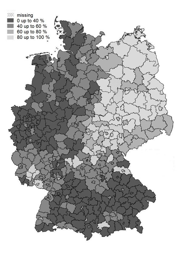
The regional differences can be seen in Figure 1 and Table 3 which depict descriptive
Figure 1: Share of 1- and 2-year-olds in subsidized care in 2015. Source: Alt et al. (2015)
statistics of the child care coverage rates on the district level. Figure 1 shows that child
care coverage rates are the highest in East Germany while the lowest can be found in the
Southern and West-Northern states. Table 3 confirms these findings for the included 318
districts. In 2011, the lowest share of children in subsidized care measured on the district
level amounted to 9.2 percent while the maximum was at 61.0 percent. The maximal value
remained stable until 2015, but the minimum almost increased by one half within 4 years.
Furthermore, the mean increased from 2011 onwards by 7.2 percentage points to 32.8
percent. Table 4 indicates how the treated districts are spread over the federal states. The
majority of Northern and Western districts belong to the treated group for which the cover-
age rate increased by more than 8.0 percentage points. In Southern states the distinction
is less obvious while most districts in East Germany belong to the control group for whom
the coverage rate increased to a lesser extent. One may be concerned that most districts
of the former GDR belong to the control group. However, a robustness check that drops
East German districts will provide similar results compared to the baseline estimates.
The idea of the difference-in-differences estimator is to compare average outcomes of
a group affected by a reform with unaffected individuals before and after the treatment
2
Figure 2 in the Appendix depicts the distribution of the growth of the child care coverage rate between
2011 and 2015. The identification of treatment and control group would be questionable in case of intense
concentration around the separation. I find that the distribution is similar to the normal distribution and
conclude that the identification strategy does not impose major problems.
IAB-Discussion Paper 2/2019 12Table 3: Coverage rates for children aged up to three years in %, district level
Minimum Maximum Mean
2011 9.2 61.0 25.6
2012 10.5 63.3 28.0
2013 11.3 63.2 29.7
2014 13.9 63.0 32.5
2015 13.0 63.1 32.8
Unweighted. Own calculations based on 318 districts.
Source: Federal Statistical Office (2011a, 2012a, 2013a, 2014a, 2015a).
Table 4: Number of districts by group membership and federal states
Federal state Control group Treatment group
Schleswig-Holstein 0 13
Hamburg 0 1
Lower Saxony 6 31
Bremen 0 1
North Rhine-Westphalia 1 46
Hesse 7 10
Rhineland-Palatinate 22 8
Baden-Württemberg 20 11
Bavaria 50 25
Saarland 1 2
Berlin 1 0
Brandenburg 13 3
Mecklenburg-Vorpommern 2 0
Saxony 6 3
Saxony-Anhalt 14 0
Thuringia 17 4
Source: Own calculations based on numbers of the
Federal Statistical Office (2011a, 2015a) from 318 districts.
comes into effect. Under the assumptions of i) parallel trends of control and treated group
in the absence of the reform, ii) the absence of anticipation effects and iii) the stable unit
treatment value assumption (SUTVA), the double difference depicts the treatment effect
(Lechner, 2011). Assumption i) can be expressed as
E(Y 0 (i, 1)|X(i), D(i, 1) = 1) − E(Y 0 (i, 0)|X(i), D(i, 1) = 1)
= E(Y 0 (i, 1)|X(i), D(i, 1) = 0) − E(Y 0 (i, 0)|X(i), D(i, 1) = 0)
where E(Y 0 (i, t) denotes the potential outcome in the absence of the treatment at time
t = 0, 1 for individual i, some covariates X(i) and the treatment status D(i, t) = 0, 1 which
is always 0 in t = 0. E(Y 1 (i, t)) is its counterpart under the reform. Assumption i) is crucial
for DD-estimation, as deviating from the common trend gives a biased estimate for
E(Y 1 (i, 1)|X(i), D(i, 1) = 1) − E(Y 0 (i, 1)|X(i), D(i, 1) = 1)
IAB-Discussion Paper 2/2019 13= E(Y 1 (i, 1)|X(i), D(i, 1) = 1) − E(Y 0 (i, 0)|X(i), D(i, 1) = 1)
− [E(Y 0 (i, 1)|X(i), D(i, 1) = 0) − E(Y 0 (i, 0)|X(i), D(i, 1) = 0)]
= E(Y (i, 1) − Y (i, 0)|X(i), D(i, 1) = 1)
− E(Y (i, 1) − Y (i, 0)|X(i), D(i, 1) = 0)
the average reform effect of interest. For the following, I simplify notation and write D(i, 1) =
D(i) and drop the individual index i. I follow the approach of Abadie (2005) by combin-
ing the DD-estimator with inverse probability weighting (IPW) to take non-parallel outcome
dynamics caused by differences in observable characteristics into account. A two step-
procedure firstly estimates weights based on the propensity P (D = 1|X) for weighting
temporal differences in the outcome. The second step gives a non-parametric mean com-
parison weighted by ρ0 which is determined parametrically:
P (D = 1|X)
E[ ρ0 Y ] = E(Y 1 (1)|D = 1 − Y 0 (1)|D = 1)
P (D = 1)
where
T −λ D − P (D = 1|X)
ρ0 =
λ(1 − λ) P (D = 1|X)P (D = 0|X)
and λ being the share of post-treatment observations (see Abadie (2005) for details). This
approach has two main advantages. Firstly, it does not met a functional form assumption
in the second stage and allows for flexibility. The second advantage concerns the com-
mon support between control and treatment group. If an observational unit does not have
common support within the other group, it can be dropped leading to higher comparability
between treated and control group - a feature that the outcome-based linear model cannot
consider.
Weighting temporal differences in the outcome is in particular relevant, as the reform not
only included the expansion of subsidized child care, but also the introduction of home care
allowances. Both treated and control group can apply for these benefits and thus, if their
outcome dynamics are the same in presence of the home care allowances , the estimated
effect only measures the effect of the child care expansion. Therefore, I furthermore rely
on defining treatment status based on the median increase in child care coverage. Using
mothers of older children as control group (e.g. Bauernschuster/Schlotter, 2015) would not
allow for minimizing the effect of the home care allowances. One might argue that control
districts for which child care increased by a lower amount are characterized by a larger
increase in receipt of home care allowances. However, Alt et al. (2015) show that bene-
fit receipt is the smallest in East Germany where most of the control districts are placed
(compare Table 4). Furthermore, I will run robustness checks with the number of public
subsidies received as outcome variable and find no systematic differences in the take-up
of public subsidies between high- and low-intensity districts.
Anticipation effects can be ruled out by not using observations directly before the interven-
tion came into force. Like previously mentioned, I only use pre-reform observations from
2011. Besides, SUTVA rules interactions between groups out. The assumption implies
that individuals should not change between groups which might in particular be relevant
for families moving from a control district to a treated district or vice versa. Due to the
IAB-Discussion Paper 2/2019 14repeated cross sections I cannot completely exclude these individuals, but I can control
for families having moved within the last 12 months. The estimates would also be biased
in case of other reforms taking place during the observational period. A major reform on
parental leave already came into force in January 2007 incentivizing mothers to return
to work at expiration of parental benefits (Bergemann/Riphahn, 2010, 2015; Kluve/Tamm,
2013; Kluve/Schmitz, 2018). However, the regulations were changed in July 2015 to make
part-time work during benefit receipt more attractive (Elterngeld Plus). Findings suggest
that dropping mothers of less than one-year-olds, who are affected by the reform, will turn
out to be robust compared to the baseline results.
3.2 Data and descriptive findings
The data is from the German Micro Census, a one percent representative sample of Ger-
man households. It contains annual information on the family background, employment
and other individual-specific characteristics. The survey conducted by the Federal Sta-
tistical Office partially rotates between chosen districts such that a district of households
stays in the sample for four years. A main advantage of the Micro Census is the detailed
information on the family composition. Hence, a child’s and partner’s characteristics can
be connected with the observational unit of interest, mothers whose youngest child is aged
up to three years old. I restrict the sample to mothers who are between 18 and 45 years
old and who live in a private household which corresponds to the main place of residence.
A further particularity of the Micro Census is the availability of not only agreed weekly work-
ing hours, but also the individuals working hour preferences. In contrast to other surveys
like the German Socio-econmic Panel (GSOEP) the question on working hours in the Micro
Census is filtered which means that before stating the amount of preferred working hours
the individual is asked if he/she wants to increase or decrease the agreed weekly working
hours conditioned on an earnings adjustment3 (for a methodological comparison of sur-
vey data on working hour preferences see Holst/Bringmann, 2016). Thus, there is also a
measure for under- (the wish for an increase of agreed hours) and overemployment (the
preference for less weekly hours).
I link the Micro Census data with statistics on the regional child care coverage rate for
children aged up to three years old from the German Federal Statistical Office on the dis-
trict level (Federal Statistical Office, 2010a, 2011a, 2012a, 2013a, 2014a, 2015a). The
child care coverage rate is measured on the cut-off date March, 1st and includes children
in subsidized care not additionally attending another care arrangement and children in
other care arrangements apart from subsidized care. Furthermore, I include measures for
the regional number of unemployed and vacancies from the German Federal Employment
Agency to calculate the labor market tightness in each district.
The final sample includes 9,668 mothers (of which 3,038 are currently employed) of chil-
dren aged up to three years old. I restrict the sample to married mothers sharing the place
of residence with their partner as the share of single mothers is too small (less than five
percent in the final sample) to account for this group.
3
Information on the preference for an hour increase (decrease) is included since 2006 (2008).
IAB-Discussion Paper 2/2019 15The variables used for estimating the propensity score described in the previous section
and their descriptive statistics are listed in Table 5: family and individual caracteristics, but
also information on the interview and the macroeconomic situation. These numbers result
after trimming observations, i.e. dropping individuals with a propensity score close (< 0.05)
to the minimum and maximum value (compare Imbens/Wooldridge (2009)). Trimming ex-
cludes 3,840 observations in the whole sample (N = 146 in the control group, N = 3, 694
in the treated group) and 1,188 individuals of the employed sample (N = 76 in the control
group, N = 1, 112 in the treated group)4 . A major threat to identification might stem from
using repeated cross-sections instead of panel data as individuals could have selected into
employment after the reform came effective. Hence, a balancing check looks at the co-
variate distribution of control and treated group over time. Additional to mean values and
standard deviations, Table 5 gives the standardized mean difference defined as the mean
difference over time divided by the square root of the average variance (see Rubin (2001)).
It rarely exceeds the critical value of 0.25 suggesting that selection over time depicts a mi-
nor problem. One can only observe substantial differences for the labor market tightness
reflecting economic growth over these last years. However, this development is similar for
low- and high-intensity districts.
Table 6 shows the mean of the child care coverage rate and of the examined outcome
variables, its standard deviation and mean differences between treated and control group
before and after the reform. The average coverage rate is weighted by the number of in-
cluded individuals living in each district and shows that less than one quarter of children
in high-intensity districts are in subsidized care before the reform came into force. More
mothers in low-intensity districts use subsidized care before the reform (negative, statis-
tically significant difference at t = 0), but high-intensity districts catch up resulting in a
positive spread at t = 15 .
As outcomes I examine the extensive and intensive margin, i.e., a dummy for employment,
agreed and preferred working hours and a binary indicator for working full-time (more than
30 hours per week). The federal Statistical Office measures employment according to the
concept of the International Labour Organization (employment for at least one paid hour or
self-employment in the week before the interview) which includes employees in maternity
protection and parental leave. Hence, I rely on the concept of realized employment and ex-
clude them. About one third of all mothers in high-intensity districts are currently employed
with an average of 24 hours per week. They prefer to slightly work more, on average one
hour per week. About 28 percent of them hold a full-time position. The last two columns of
Table 6 give the differences in means between treated and control group before and after
the reform. At t = 0 employment rates in high- and low-intensity districts differ significantly,
but the difference vanishes after the reform. Concerning the intensive margin, one cannot
detect any strong variation across groups and time for all measures. Hence, descriptive
findings suggest a positive link between the expansion of subsidized child care and the
employment status, but no relation to the intensive margin.
4
Histograms of the propensity score before and after trimming by group membership can be found in the
appendix.
5
Note that these are unconditional numbers that cannot give information on actual take-up of a child care
slot on the individual level.
IAB-Discussion Paper 2/2019 16Table 5: Descriptive statistics by group membership
Whole sample Currently employed sample
d = 0, t = 0 d = 0, post − pre d = 1, t = 0 d = 1, post − pre d = 0, t = 0 d = 0, post − pre d = 1, t = 0 d = 1, post − pre
Variable Mean sd Std. mean diff. Mean sd Std. mean diff. Mean sd Std. mean diff. Mean sd Std. mean diff.
Age of youngest child 0.985 0.805 -0.024 0.989 0.818 -0.035 1.341 0.682 0.102 1.354 0.702 0.090
Number of children 1.951 0.999 -0.111 1.971 1.042 -0.112 1.878 0.942 -0.125 1.922 1.068 -0.122
Age 32.79 5.027 -0.015 32.96 5.237 -0.015 33.81 4.955 -0.068 34.03 5.194 -0.090
Migration background:
none 0.881 0.323 -0.039 0.821 0.384 0.025 0.925 0.264 0.042 0.891 0.312 0.057
from EU country 0.033 0.178 0.088 0.051 0.219 0.046 0.030 0.172 0.011 0.047 0.211 -0.032
no EU country 0.086 0.280 -0.016 0.129 0.335 -0.062 0.045 0.207 -0.066 0.062 0.242 -0.046
Job position:
Self-employed - - - - - - 0.113 0.317 -0.126 0.120 0.326 -0.149
Civil servant - - - - - - 0.066 0.249 0.074 0.082 0.275 0.009
White-collar worker - - - - - - 0.707 0.455 0.067 0.690 0.463 0.141
Blue-collar worker - - - - - - 0.100 0.300 -0.053 0.096 0.295 -0.134
Others - - - - - - 0.013 0.115 0.022 0.011 0.106 0.108
Tenure - - - - - - 6.837 5.955 0.037 6.996 6.032 -0.124
Net individual income 762.1 793.0 0.193 784.0 864.8 0.196 1110.0 948.2 0.240 1257.1 1009.9 0.112
Educational degree:
Lower secondary school 0.219 0.414 -0.059 0.203 0.403 -0.150 0.173 0.378 -0.046 0.136 0.343 -0.096
Middle secondary school 0.376 0.484 0.004 0.333 0.471 -0.029 0.363 0.481 0.047 0.353 0.478 -0.065
High school 0.405 0.491 0.045 0.464 0.499 0.141 0.465 0.499 -0.011 0.511 0.500 0.124
Inactive partner 0.051 0.220 -0.046 0.062 0.242 -0.039 0.049 0.217 -0.143 0.057 0.231 -0.138
Job position:
Self-employed 0.124 0.330 -0.093 0.113 0.316 -0.063 0.164 0.370 -0.170 0.147 0.355 -0.147
Civil servant 0.043 0.203 0.071 0.045 0.208 0.053 0.051 0.219 0.097 0.061 0.239 0.015
White-collar worker 0.488 0.500 0.118 0.516 0.500 0.165 0.477 0.500 0.147 0.492 0.500 0.289
Blue-collar worker 0.279 0.449 -0.073 0.248 0.432 -0.150 0.245 0.430 -0.029 0.224 0.417 -0.156
Others 0.015 0.120 -0.030 0.016 0.126 -0.030 0.015 0.120 0.001 0.020 0.140 -0.067
Employment status:
Full-time 0.906 0.292 -0.020 0.864 0.343 0.073 0.897 0.304 0.040 0.865 0.341 0.091
Part-time 0.032 0.177 0.058 0.051 0.220 -0.031 0.044 0.205 0.064 0.054 0.226 0.028
Marginal employment 0.011 0.103 0.040 0.022 0.148 -0.061 0.010 0.100 0.006 0.024 0.153 -0.059
Labor market tightness (district) 0.022 0.011 0.449 0.019 0.009 0.511 0.021 0.011 0.466 0.019 0.009 0.507
East Germany 0.171 0.376 -0.009 0.070 0.255 0.004 0.224 0.417 0.009 0.096 0.295 0.019
Quarter of interview
1 0.261 0.439 -0.039 0.232 0.422 -0.005 0.275 0.447 -0.015 0.229 0.421 0.055
2 0.249 0.433 -0.027 0.263 0.440 -0.064 0.249 0.433 0.004 0.258 0.438 -0.055
3 0.238 0.426 0.036 0.256 0.437 -0.041 0.224 0.417 0.012 0.254 0.435 -0.079
4 0.251 0.434 0.030 0.249 0.432 0.107 0.251 0.434 -0.001 0.259 0.439 0.076
Interview part
IAB-Discussion Paper 2/2019
Head of household 0.193 0.394 0.011 0.217 0.412 0.013 0.205 0.404Table 6: Mean outcomes and coverage rate by group membership
d = 1, t = 0 Difference in means
Treated-control group
Variable Mean sd N t=0 t=1
All: Coverage rate (weighted) % 22.04 (8.06) 2,233 -2.76*** 2.8***
Employed: Coverage rate (weighted) % 22.95 (9.10) 706 -3.33*** 1.87***
Employed of which: 0.3515 0.4776 2,233 -0.0364*** 0.0013
Agreed hours 24.00 13.13 706 0.48 0.49
Preferred hours 25.13 13.11 706 0.53 0.26
Full-time 0.2847 0.4516 706 -0.0138 -0.0115
∗p < 0.1, ∗ ∗ p < 0.05, ∗ ∗ ∗p < 0.01. The sample includes 18 to 45 years old, married mothers of up to three-year-olds.
Source: Own calculations based on data from the German Micro Census, the Federal Statistical Office (2011a, 2015a)
and the Federal Employment Agency.
4 Estimation results
4.1 Main results
Table 7 shows the baseline estimation results for the whole sample and different subgroups
according to Abadie (2005). Standard errors consider the two-step estimation procedure
by bootstrapping taking clusters on the district level into account.
In general, districts with a large increase of the coverage rate experience a rise of both
the employment rate and working hours compared to districts with a lower expansion of
child care. The reform effect amounts to an increase of the employment rate of ten per-
centage points. Agreed and preferred weekly hours increase by 4.1 and 4.0 (17 percent
of the pre-reform mean) respectively. Although the estimates lack statistical significance
on conventional levels, they are close to it. Interestingly, these findings suggest an almost
equal adjustment of agreed and preferred hours such that the effect on the mismatch size
is close to zero. The similar adjustment also implies that the effect is not only driven by in-
voluntarily underemployed mothers who adjust agreed to preferred working hours, but that
both distributions change. They suggest (see histograms of agreed and preferred working
hours in the Appendix) a shift from marginal employment (categorized as up to 15 hours
per week) to part-time work (between 16 and up to 30 hours per week). One can also
observe a decrease at the upper part of the hour distribution. However, it contributes less
to the average effect due to the lower share of full-time working mothers. Further estima-
tion results not shown in Table 7 demonstrate that the share of under- and overemployed
mothers is not significantly affected. Hence, the overall positive effect on working hours
is driven by a shift from marginal to part-time employment which also shows up in a not
affected share of full-time employed.
The estimates vary strongly for other subgroups. Mothers with high school degree show
a strong response to the reform by a rise in the employment rate of about 14 percentage
points. Mothers with a lower degree are characterized by small or even negative effects that
are not statistically significant, but sample size is considerably smaller for those subgroups.
Havnes/Mogstad (2011) also find larger effects for better educated women. However, this
difference is weaker pronounced as the general reform effect also turns out to be smaller.
IAB-Discussion Paper 2/2019 18I also condition on the individual net income that includes public allowances and capital
income. Interestingly, mothers with low- to middle income (up to 1,000 Euro) seem to have
benefitted more from the reform as these mothers show a large rise of employment (11
percentage points) and especially of hours (11 and 12 hours per week for agreed and pre-
ferred hours). For mothers with higher income the effects are as well positive but lower
and not statistically significant. The latter finding provides evidence for a stronger income
or weaker substitution effect for this group, i.e. mothers with higher income have a higher
preference for leisure. The variation of the estimates for income- and education-based sub-
groups do not necessarily contradict as the net income also depicts other income sources,
tax incentives and the employment status (marginal employment, full- or part-time work).
Hence, mothers with lower secondary school degree can also belong to the group with
higher net income. Besides, the small group of employed women with lower secondary
school degree contributes less to the average effect on working hours.
As Weber/Zimmert (2017) show socio-economic characteristics are correlated with the type
of an working hour discrepancy. Therefore, heterogenous effects can indicate how uncon-
strained, under- or overemployed mothers adjust preferred and agreed working hours. The
authors find that overemployment is linked to better education, jobs of higher occupational
autonomy and higher wages while the opposite holds for underemployment. The estimates
do not suggest deviating adjustment mechanisms for preferred and agreed working hours
for different subgroups which supports the consideration of an equal shift along the distri-
bution.
Finally, the last rows show that the effects do not strongly vary for different age groups.
4.2 Robustness
Table 8 contains different robustness checks. Firstly, for investigating the common trend
assumption which is crucial for DD-estimation I check whether the time trend before the
reform is the same for districts with a high and smaller increase of the coverage rate. I
test a specification by introducing a placebo reform with the pre-reform period being 2010
(t = 0) and the post-reform period 2011 (t = 1). The estimates prove not to statistically
significantly differ from zero (Panel D, first row). Hence, close to the reform treated and
control group show a similar time trend. Since the reform also included the introduction
of home care allowances, a second test uses the number of received public subsidies
as outcome variable. Unfortunately, an explicit information on the receipt of home care
allowances is not available. The last rows of Panel D demonstrate that treated and control
group do not show a statistically different pattern concerning the receipt of public subsidies
suggesting that the baseline estimate in table 7 is likely to solely measure the effect of the
expansion of subsidized child care.
The next specification (Panel A) uses the median of the increase of the coverage rate for
redefining the treatment and control group. As expected, the effect is less pronounced
compared to using a clearer cut as in the main specification in Table 7.
Other checks deviate form the baseline by changing the sample composition (Panel B). The
reform demonstrates to have a similar, but stronger effect when using only West German
districts. Employment of mothers living in high-intensity West-German districts increases
by 12 percentage points, their working hours by about seven hours per week. Again, the
IAB-Discussion Paper 2/2019 19Table 7: Main estimation results
Employed (binary) Agreed hours Preferred hours Full-time
Panel A: Whole sample
Whole sample 0.1006*** 4.1228 3.973 0.0010
(0.0317) (2.6386) (2.6727) (0.05583)
N 9,668 3,038 3,038 3,038
Panel B: Heterogeneities
Education:
Lower secondary school 0.0780 -1.2869 -0.4762 -0.1103
(0.0624) (5.7127) (6.2163) (0.0992)
N 1,810 399 399 399
Middle secondary school 0.0128 3.4284 3.5950 0.0322
(0.0645) (4.5154) (4.8162) (0.0877)
N 3,391 1,066 1,066 1,066
High school 0.1354*** 4.9319 5.4396 -0.0106
(0.0467) (4.0373) (4.0415) (0.0872)
N 4,355 1,436 1,436 1,436
Individual net income:
< 1000 Euro/month 0.1149*** 10.9015*** 12.2056*** 0.0436
(0.0340) (2.7107) (3.1427) (0.0376)
N 6,375 1,377 1,377 1,377
≥ 1000 Euro/month 0.0946 1.2796 1.3972 -0.0090
(0.0696) (4.1941) (4.2007) (0.0943)
N 3,188 1,620 1,620 1,620
Age:
< 35 years 0.1008** 3.4583 3.7562 -0.0570
(0.0401) (3.4481) (3.6123) (0.0737)
N 6,110 1,734 1,734 1,734
≥ 35 years 0.0951 3.5326 3.1989 0.0172
(0.0600) (3.9087) (4.0019) (0.0845)
N 3,497 1,253 1,253 1,253
∗p < 0.1, ∗ ∗ p < 0.05, ∗ ∗ ∗p < 0.01. Standard errors (in columns) are bootstrapped with 1,000 replications
considering clusters on district level. The sample includes 18 to 45 years old, married mothers of up to three-year-olds.
Agreed and preferred hours are measured on weekly basis.
Source: Own calculations based on data from the German Micro Census, the Federal Statistical Office (2011a, 2015a)
and the Federal Employment Agency.
share of full-time employed is not significantly affected. These findings show that the overall
effect for both East and West Germany turns out to be robust considering any systematic
differences between districts of the former GDR and West German districts implying no
major problem for including East Germany in the baseline analysis. Dropping mothers of
children younger than one year old leads to a slightly larger effect for all outcomes. Hence,
the parental leave reform of 2015 that affected mothers with children in this age group is
not supposed to drive the results. As mothers working in a child care facility might be
differently affected by the reform, they are excluded in another specification which only
slightly changes the estimates. Secondly, I test for selective migration by excluding those
having changed their place of residence within the last twelve months. These estimates
are also similar to the baseline results of Table 7.
A last specification in Panel C varies by running parametric regressions with OLS of the
form:
yit = γ1 postit + γ2 treatit + γ3 postit ∗ treatit + δXit + µit
with post being one in t = 1 and zero otherwise, treat depicting treatment status and their
interaction giving the estimate of interest, γ3 . X includes the same covariates as for semi-
IAB-Discussion Paper 2/2019 20parametric estimation and the standard errors are clustered on the district level. Although
the estimates are clearly smaller compared to the baseline according to Abadie (2005),
their signs and statistical relevance are the same.
Table 8: Robustness
Employed (binary) Agreed hours Preferred hours Full-time
Panel A: Treatment definition
Median division 0.0631** 3.1862 2.8345 0.0176
(0.0252) (2.0715) (2.0884) (0.0408)
N 13,246 4,224 4,224 4,224
Panel B: Sample composition
West Germany 0.1209*** 7.2871** 7.0683** 0.0800
(0.0399) (3.2207) (3.2726) (0.0639)
N 8,838 2,685 2,685 2,685
Without 1-year-olds 0.1440*** 5.6205* 5.279* 0.0586
(0.0478) (2.8811) (2.9714) (0.0599)
N 6,338 2,725 2,725 2,725
Without childminders 0.0863*** 3.7500 3.4963 0.0023
(0.0314) (2.6609) (2.7514) (0.0574)
N 9,692 3,044 3,044 3,044
Without families having moved 0.1064*** 3.5563 4.0309 -0.0284
(0.0340) (2.7094) (2.8439) (0.0586)
N 8,660 2,784 2,784 2,784
Panel C: Parametric form
Parametric form 0.0304* 1.0072 0.5826 0.0359
(0.0171) (0.7353) (0.7792) (0.0282)
N 9,668 3,038 3,038 3,038
Panel D: Common trend
Placebo reform 0.0088 -0.6104 0.3298 -0.0387
(0.0322) (2.2377) (2.4367) (0.0477)
N 9,574 3,175 3,175 3,175
Whole sample: Employed:
Number of public subsidies Treated, t = 0: Mean AT T Treated, t = 0: Mean AT T
0.8433 -0.0102 0.6275 0.0791
(0.7582) (0.0625) (0.5675) (0.0880)
9,665 3,037
∗p < 0.1, ∗ ∗ p < 0.05, ∗ ∗ ∗p < 0.01. Standard errors (in columns) are bootstrapped with 1,000 replications
considering clusters on district level. The sample includes 18 to 45 years old, married mothers of up to three-year-olds.
Agreed and preferred hours are measured on weekly basis.
Source: Own calculations based on data from the German Micro Census, the Federal Statistical Office (2011a, 2015a)
and the Federal Employment Agency.
5 Conclusion
This paper provides empirical evidence for the causal effect of subsidizing early child care
on maternal labor market outcomes. It exploits the staggered expansion of early child care
provision in Germany culminating in a legal claim for a child care slot introduced in 2013.
The presented semi-parametrically estimated intention-to-treat effects suggest a strong im-
pact of ten percentage points on the maternal employment rate and less significantly of four
on agreed and preferred weekly working hours. Besides, the share of full-time employed
women does not change in response to the reform which might result from limited provision
IAB-Discussion Paper 2/2019 21You can also read