INDONESIA SELECTED ISSUES - International Monetary Fund

IMF Country Report No. 19/251

 INDONESIA
 SELECTED ISSUES
July 2019
 This paper on Indonesia was prepared by a staff team of the International Monetary Fund
 as background documentation for the periodic consultation with the member country. It
 is based on the information available at the time it was completed on June 17, 2019.

 Copies of this report are available to the public from

 International Monetary Fund • Publication Services
 PO Box 92780 • Washington, D.C. 20090
 Telephone: (202) 623-7430 • Fax: (202) 623-7201
 E-mail: publications@imf.org Web: http://www.imf.org
 Price: $18.00 per printed copy

 International Monetary Fund
 Washington, D.C.

 © 2019 International Monetary Fund

INDONESIA
 SELECTED ISSUES
June 17, 2019

 Approved By Prepared By Calixte Ahokpossi, Agnes Isnawangsih,
 Asia and Pacific Md. Shah Naoaj (all APD), Ting Yan (COM), Baoping Shang
 Department (FAD), Heedon Kang (MCM), and Manasa Patnam (SPR)

 CONTENTS

 EXCHANGE RATE AND TRADE DYNAMICS IN INDONESIA: CONNECTING
 THE DOTS ________________________________________________________________________________ 4
 A. Exchange Rate and Trade Balance: Recent Trends ____________________________________ 4
 B. Data and Empirical Methodology _____________________________________________________ 7
 C. Results________________________________________________________________________________ 8

 References _______________________________________________________________________________ 15

 FIGURE
 1. Exchange Rate and Trade Fluctuations: Recent Trends _______________________________ 5

 TABLES
 1. Import Price: Pass-Through of Exchange Rate and Commodity Price _________________ 9
 2. Export Price: Pass-Through of Exchange Rate and Commodity Price ________________ 11
 3. Import and Export Volume Response to Prices ______________________________________ 11

 INDONESIA’S GROWTH-AT-RISK ______________________________________________________ 17

 References _______________________________________________________________________________ 25

 FIGURES
 1. Financial Condition Index ____________________________________________________________ 20
 2. Macrofinancial Vulnerability Index ___________________________________________________ 20
 3. Quantile Regression Results _________________________________________________________ 21
 4. Growth-at-Risk Results ______________________________________________________________ 21

INDONESIA

 TABLE
 1. List of Macrofinancial Variables for GaR Analysis ____________________________________ 18

 APPENDICES
 I. Data Source _________________________________________________________________________ 22
 2. Parametric Estimation of Future Growth Distribution ________________________________ 23

 IMPACT OF MONETARY POLICY COMMUNICATION IN INDONESIA ________________ 26
 A. Transparency and Clarity ____________________________________________________________ 26
 B. Predictability ________________________________________________________________________ 28
 C. Impact on Market Rates _____________________________________________________________ 29

 FIGURES
 1. Press Releases Words and Paragraphs _______________________________________________ 28
 2. Predictability of Interest Rate Decision ______________________________________________ 28

 TABLES
 1. Impact of Monetary Policy Surprise and Anticipation ________________________________ 29
 2. Impact of Press Release on Market Rates ____________________________________________ 30
 3. Impact of Monetary Policy Reports on Market Rates ________________________________ 31

 APPENDICES
 I. Data Source _________________________________________________________________________ 32
 II. Impact of Press Release and Monetary Policy Report ________________________________ 33
 III. Description of Analytical Approaches ________________________________________________ 34

 OPERATIONALIZING A MEDIUM-TERM REVENUE STRATEGY IN INDONESIA ______ 36
 A. The Context _________________________________________________________________________ 36
 B. Key MTRS Reforms __________________________________________________________________ 38
 C. Complementary Reforms ____________________________________________________________ 44
 D. Sequencing and Phasing ____________________________________________________________ 45
 E. Conclusion __________________________________________________________________________ 47

 References _______________________________________________________________________________ 53

 BOXES
 1. CIT and Tax Competition ____________________________________________________________ 48
 2. Public Investment Efficiency _________________________________________________________ 49

2 INTERNATIONAL MONETARY FUND

INDONESIA

FIGURES
1. Government Revenues and Collection Efficiencies ___________________________________ 37
2. Revenue Gain from Sequencing and Phasing of Reforms—An Illustrative Scenario __ 46

TABLES
1. Doing Business Ranking _____________________________________________________________ 38
2. Key Tax Policy and Administration Reforms _________________________________________ 50
3. Reform Sequencing and Phasing ____________________________________________________ 51
4. An Action Plan in the Near Term ____________________________________________________ 52

 INTERNATIONAL MONETARY FUND 3

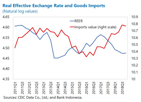
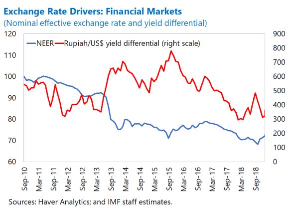
INDONESIA

EXCHANGE RATE AND TRADE DYNAMICS IN
INDONESIA: CONNECTING THE DOTS1
This paper provides an overview of the exchange rate and trade dynamics in Indonesia. Using data on
monthly export and import price and volume at the sectoral level, the paper estimates pass-through
effects of exchange rate changes to trade price and volume. Results indicate adjustment frictions that
depend on the source of the exchange rate fluctuation and the degree of integration in global value
chains. Overall, combining price and volume effects, we find that a 10 percent depreciation in the
exchange rate is associated with a rise in the goods net-exports of up to 1.6 percent of GDP.

A. Exchange Rate and Trade Balance: Recent Trends

1. Movements in exchange rates play an important role in determining how a country’s
trade balance adjusts in response to both external and domestic shocks. Exchange rates
typically act as a shock absorber, in the sense that in response to an external shock, a depreciation
should boost exports through the competitiveness channel and reduce imports as they become
more expensive relative to domestic goods.2 However, recent evidence from both emerging and
advanced countries suggests that the transmission of exchange rate changes to trade price and
quantities, through the expenditure-switching channel,3 may be incomplete (see for example, Campa
and Goldberg 2005). We examine this issue for Indonesia and attempt to, first, uncover a pattern
from recent trends in both exchange rates and trade movements. Figure 1 below charts, since 2011,
the movements in exchange rates in relation to both the terms of trade (proxy for real-sector
fundamentals) and interest rate differentials (proxy for carry-trade attractiveness in international
financial markets) as well as value of goods exports/imports. We see that, after a period of decline
following the taper tantrum in 2013, goods imports have rebounded and steadily increased in the
past few years despite a sharp depreciation of the rupiah since mid-2017. Following the tightening
of global financing conditions in 2018, which put pressures on financial flows to Indonesia, the
rupiah depreciated by about 6 percent in real effective terms. However, during the same period,
imports surged both in value and volume terms by approximately 20 percent and 8 percent year-
on-year respectively. On the other hand, exports moved more in line with recent changes in the
exchange rate, growing in value by 7 percent in 2018.

1 Prepared by Manasa Patnam (SPR).
2 See Obstfeld (2001) and Engel (2002) for a survey.
3 The expenditure-switching effect, the focus of this paper, refers to the shifting of domestic consumption away from
foreign goods towards domestic goods because of trade price changes. In addition to this, there may also be an
expenditure-changing or wealth effect which reflects the reduction in purchasing power associated with a weaker
currency, leading to a compression of domestic demand and thereby of imports.

4 INTERNATIONAL MONETARY FUND

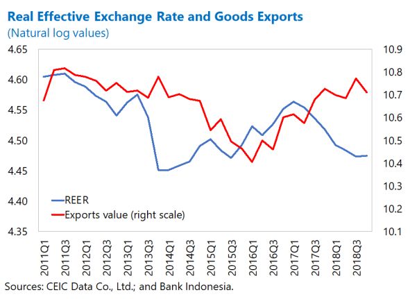
INDONESIA

2. Exchange rate movements appear to have increasingly diverged from trade-related
pressures, indicating a possible disconnect from fundamentals. An examination of the drivers of
exchange rate reveals that movements in the
nominal exchange rate have recently diverged Correlation of Exchange Rate with Terms of Trade and
 Interest Rate Differentials 1/
from real-sector related fundamentals. For
instance, as shown in Figure 1 and text table, the 2011-2014 2015-2018
correlation between the terms of trade and NEER,
has switched from positive (2010−2014) to Correlation between ToT and NEER 0.67 -0.32

negative (2015−2018) over the recent half of this Correlation between IRD and NEER -0.65 0.49

decade. In contrast, we find that the opposite
pattern holds for the relationship between the 1/ ToT refers to terms of trade, NEER to nominal effective
 exchange rates, and IRD to the Indonesia-U.S. interest rate
exchange rate and movements in the financial differential (in bps). All pairwise correlation coefficients are
sector (proxied by the Indonesia-U.S. interest rate signficant at the 5% level.

differential), where the correlation has turned from
negative to positive.

 Figure 1. Indonesia: Exchange Rate and Trade Fluctuations: Recent Trends

 INTERNATIONAL MONETARY FUND 5

INDONESIA

3. The volatility of exchange rates appears higher than fundamentals. The estimated
standard deviation of both the PPI-based REER and
NEER index (during 2010:Q1-2018:Q4) is strictly
above the standard deviation of the terms of trade
index by approximately 4 standard deviations. In
addition, the PPI-based real exchange rate tracks
very closely the nominal exchange rate at the
monthly frequency and displays a similarly large
persistence and volatility as the nominal exchange
rate. These facts suggest that the exchange rate
displays both high and “excess volatility” appearing
therefore to be disconnected from fundamentals
(see Chari and others, 2002 and Baxter and
Stockman, 1989).

4. High exchange rate volatility, in excess of the volatility of fundamentals, is intrinsically
linked to a limited pass-through of exchange rates to trade prices. Empirical evidence has
shown that the excess volatility of real and nominal exchange rates is associated with limited pass-
through effects of exchange rate changes to trade and consumer prices (Devereux and
Engel, 2002).4 This would imply that, both, depending on the nature of the shock and transmission
mechanism, the change in the nominal exchange rate may not lead to a full substitution between
domestic and foreign goods because of slow-changing relative prices of home and foreign goods.

5. The literature has examined several reasons related to both the source of shock and
transmission mechanism to understand why pass-through effects of exchange rate changes to
trade prices may be limited. These explanations can be broadly divided into those concerning the
nature of the exchange rate shock, which creates different types of fluctuations, and those related to
the transmission mechanism, which mutes the effect of volatile exchange rate fluctuations on local
prices and quantities. In terms of the shock process, it has been posited that shocks emanating from
international asset demand generate large and volatile exchange rate fluctuations that have small
effects on the rest of the economy, because of financial frictions compared to productivity/demand
or monetary shocks (Devereux and Engel, 2002; Forbes and others, 2018). The reasons why financial
market shocks may be less impactful hinge on distortions within the micro-foundations of the
international markets such as the presence of noise traders with limits to arbitrage, financial
frictions, and time-varying risk premium (see Itskhoi and Mukhin, 2017).

4 This means that the relationship between the equilibrium exchange rate and real-economy shocks are amplified by
the presence of frictions related to firms, speculative activity in financial markets and market structure of international
trade. For early insights on this see Krugman (1989) who argues that firms face significant sunk cost frictions and do
not react to exchange rate changes that lie within a range, preferring a ‘wait and see’ approach, which prevents them
from adjusting their prices and volumes instantaneously. Further over time, an increased volatility of exchange rates,
partly from excessive speculation in international financial markets, could widen this range and further weaken firms’
responsiveness.

6 INTERNATIONAL MONETARY FUND

INDONESIA

6. In terms of the transmission mechanism the literature has emphasized the role of
price-setting, the structure of international trade markets and demand preferences. For
instance, there may be a significant home-bias in consumption that may weaken the expenditure
switching effects of exchange rate changes from limited adjustment of trade quantities.
Alternatively, local currency pricing or pricing to market with markup adjustment may limit the
responses of trade prices to exchange rate movements. Finally, the global integration of trade
markets, where import and export production process are no longer isolated and instead linked
though complex supply-chain arrangements, may create offsetting impacts on prices that may net
out the price effects in the aggregate.

7. To understand whether the exchange rate movements and trade flows are
disconnected in recent times, we estimate the sectoral pass-through effect of exchange rate
changes on trade prices and quantities. Using data on monthly trade prices and volumes at the
sectoral level, the paper first examines if, and to what extent, the pass-through effects are limited.
Next it examines a few specific channels, especially relevant for Indonesia, that may drive these
effects. Depending on the sector’s orientation and structure, limited pass-through can arise from
deeper involvement in global value chains and foreign currency invoicing. In addition, these effects
can be asymmetric such that the magnitude of pass-throughs may vary in response to exchange
rate appreciations and depreciations.

B. Data and Empirical Methodology

8. We use sectoral data on import and export volume and prices at a monthly frequency
to estimate six- and twelve-month pass-through effects. Trade value and volume data are
obtained from Statistics Indonesia (BPS) at the SITC (revision four) sectoral classification. Real
effective exchange rate data is from BIS. Monthly commodity price index5 is from the IMF and data
on global value chains is obtained from the OECD Trade in Value database.

9. Our estimation of aggregate trade-related pass-through effects, accounts from the
possible heterogeneity of these effects across sectors. Estimates obtained from pooling all
sectoral data can typically suffer from an “aggregation bias,” if the price volatility is driven by sectors
that experience relatively higher or lower elasticity. For instance, we would expect the results to be
upward biased in high price volatility sectors are relatively inelastic. This insight was developed by
Imbs and Mejan (2015) who show how aggregate elasticities obtained from combining disaggregate
effects differ substantially from those obtained based on examining purely aggregate relationships.

5 Theindex is used to identify (approximately) terms of trade shocks to commodity related exports/imports and
represents four broad commodity asset classes: (1) energy, (2) agriculture, (3) fertilizers, and (4) metals and is a
weighted average of 68 global commodity prices. The weight is calculated based on the global import share over a
3-year period (2014−2016) and is normalized to 100 at year 2016 prices.

 INTERNATIONAL MONETARY FUND 7

INDONESIA

10. Using sectoral monthly data on trade flows, we augment the exchange rate pass-
through equation with commodity price shocks and account for the asymmetric response to
shocks. We attempt to eliminate the effect of nominal price rigidities on pass-through estimates by
focusing on the six- and twelve-month changes of trade prices and quantities,6 where subscript ct
denotes the cumulative change of all variables (trade prices, quantities, exchange rate and
commodity price) between time t and the previous six or twelve months for sector i. The
specification also mitigates bias from other (unobserved) economic factors that may be correlated
with both import/export prices and ER/commodity shocks by conditioning on quarterly time effects
( ). These time dummies can capture at the quarterly level, for instance, policy actions in response
to exchange rate fluctuations or movements in other real-economic variables that are not explicitly
included in the specification. In sum, the exchange rate ( ) and commodity price ( ) pass-through for
the dependent variable, import prices ( ) expressed in local currency, can be specified as.7

 + ∆ 
 ∆ , = ⏟ +
 + − ∆ 
 −
 + + ⏟ +
 ∆ + − ∆ 
 −
 + + , 
 ℎ 

The overall pass through can then be obtained by aggregating sector-wise pass-through coefficients
based on their shares ( + = ∑ + and − = ∑ − ). A similar specification is employed for
export prices expressed in foreign currency. In the next step we use the observed cumulative price
changes to predict quantity response, while similarly conditioning on quarter specific time effects.

C. Results

11. Results indicate that there is considerable asymmetry and sectoral heterogeneity in
the pass-throughs of exchange rate on import and export prices. The overall pattern that
emerges from the estimated disaggregated effects below is that (i) trade prices are on average more
responsive, i.e., have higher estimated pass-throughs, to exchange rate shocks relative to
commodity price shocks; (ii) the exchange rate pass-through coefficient of import prices is higher
than that of export prices; (iii) both export and import price pass-throughs vary by the nature of the
shock with appreciations (depreciations) linked to stronger import (export) price changes; and
(iv) sectoral price pass-throughs are dispersed, with the largest importing and exporting sectors
having weak price responses to exchange rate fluctuations over a six-month horizon.

12. Import prices adjust well to exchange rate fluctuations with the effects being stronger
for appreciation episodes. Table 1 reports the estimated import-price pass-through coefficients by

6 Gopinath and others (2010) exploit good level data and identify pass throughs using cumulative changes in the log
of the bilateral nominal exchange rate over the duration for which the previous price was in effect. However, since
our data is at the sectoral level (combining several good) we are unable to identify discrete price changes and
therefore focus on cumulative changes, assuming that rigidities last between six to twelve months. The median
duration for trade price rigidity is estimated to be around 9−12 months (see Gopinath and Rigobon, 2008) but
commodity goods can have lower durations.
7 In this specification, denotes the log of real effective exchange rate and denotes the log of commodity price
index. Import and export prices are derived based on their respective values and volumes. Import prices. , are
expressed in Indonesian rupiah and deflated by the consumer price index. Export prices are expressed in U.S. dollars
and deflated by the foreign consumer price index. Import and export volumes are also expressed in logs.

8 INTERNATIONAL MONETARY FUND

INDONESIA

sector and differentiated by the type of shock (exchange rate vs commodity price) as well as by
horizon. First, focusing on the six-month horizon we find that overall, across sectors, a 10 percent
increase in exchange rate (appreciation) is associated with an import price decrease of 5.7 percent.
On the other hand, a 10 percent increase in commodity prices is associated with an import price
increase of 4.6 percent. The aggregate effects however mask important directional and sector-
specific effects. For instance, a 10 percent appreciation of the exchange rate is associated with a
decline in import prices by 8 percent, whereas a similar magnitude of depreciation results in only a
3 percent increase in import prices. In terms of sectoral effects, we find that the sector with the
largest import share, accounting on average for 32 percent of total imports, (machinery and
transport equipment) has a very low sensitivity to exchange rate (coefficient of -0.04) movements
compared to other top importing sectors which have significantly higher pass-throughs (coefficient
on average of -0.6). Turning to the twelve-month horizon, we see a general improvement in the
import price sensitivities, with a 10 percent increase in exchange rate (appreciation) associated with
an import price decrease of 7 percent, which indicates that the pass-through of exchange rates to
import prices have a delayed effect. Most notably, the largest importing sector, which had almost
negligible pass-throughs over the six-month horizon, increases its sensitivity to 6 percent (following
a 10 percent exchange rate change) at the twelve-month horizon. This could be explained by time-
lags in pricing and delivery and settlement delays. As before, we find a similar pattern of
heterogeneity with twelve-month pass-throughs being stronger for appreciation and commodity
price declines.

 Table 1. Indonesia: Import Price: Pass-Through of Exchange Rate and Commodity Price 1/

 Share in Exchange Rate Pass-Through Commodity Price Pass-Through
 Imports 6-month 12-month 6-month 12-month

 Food and live animals 8.4% -0.36 -0.66 -0.15 0.32
 Beverages and tobacco 0.5% -5.90 -3.93 -1.23 -0.96
 Crude materials 5.1% -1.47 -0.81 -0.28 0.09
 Mineral fuels, lubricants 19.4% -1.07 -1.00 0.89 0.87
 Animal and vegetable oils and fats 0.1% 2.79 2.57 0.24 0.29
 Chemical 13.8% -1.04 -0.65 0.20 0.17
 Manufactured goods 16.0% -0.23 -0.37 1.27 0.69
 Machinery and transport equipment 31.7% -0.04 -0.57 0.21 0.67
 Miscellaneous manufactured articles 4.5% 0.02 -1.37 0.04 0.22
 Other 0.4% -9.24 -0.73 4.50 11.63

 Total 100% -0.57 *** -0.70 *** 0.46 *** 0.60 ***

 Asymmetric effects:
 + (Appreciation/commodty price increase) -0.80 * -1.01 *** 0.33 0.58 ***
 - (Depreciation/commodty price decrease) -0.31 ** -0.43 ** 0.53 *** 0.70 **

 1/ The estimation sample period is between 2011–2018. Gray shaded cells for individual sectoral indicate effects that are not
 significant at the 10% level. Significance for aggregate effects are as follows: *** indicates significance at the 1% level; ** at the
 5% level and * at the 10% level. 6-month refers to a cumulative horizon of six months; 12-month to a cumulative horizon of one
 year. Asymmetric effects are aggregated from the (unreported) sector-wise differentiated effects. Sectoral import and export
 shares are an average over the sample period.

 INTERNATIONAL MONETARY FUND 9

INDONESIA

13. The price sensitivity of export prices to exchange rate shocks is generally lower than of
imports and concentrated over shorter horizons and during episodes of depreciation. Table 2
reports the estimated export-price pass-throughs by sector and differentiated by the type of shock
(exchange rate vs commodity price) as well as by horizon. Overall, across sectors, a 10 percent
increase in exchange rate (commodity-prices) is associated with increasing export prices (in foreign
currency) by 4 percent (2 percent) at the six-month horizon compared to 1.5 percent (3 percent)
over the twelve-month horizon. One explanation for the result that exports prices have lower
estimated pass-through coefficients than import prices could be that firms set export prices in a
dominant currency (mostly the dollar) and are therefore unable to change frequently their prices in
response to exchange rate changes. There is however considerable asymmetry and heterogeneity in
the distribution of these effects across sectors and by type of shocks.8 Depreciations and
commodity-price declines are associated with higher pass-throughs compared to appreciations and
commodity price increases. We find a large dispersion of these effects across sectors, with the
largest exporting sector having insignificant pass-throughs for exchange rate changes but significant
pass-through effects for commodity price changes (on average 4 percent increase to a 10 percent
increase in commodity prices).

14. With regards to estimation, it should be noted that pooled estimates of the overall
aggregate effect are significantly downward biased. Results from a specification that pools all
sectors reveals an aggregate import and export pass-through coefficient of -1.65 and 0.06,
respectively. As discussed above there is substantial heterogeneity in both the sectoral share in total
export/import value and the related sector-specific volume effects to price changes. The downward
bias suggests the presence of sectors whose prices experience large price changes, but which are
relatively more elastic.

15. The volume of both imports and exports are fully responsive to price changes. For a
given level of price change, overall, we find that, for both exports and imports, the six-month
adjustment to quantities is strong with aggregate elasticities close to one (Table 3). Import
quantities adjust one-on-one to change in import prices, over all horizons. For exports, the effect is
strong over the six-month horizon but weaker over time. There is still some sectoral variation in the
distribution of these effects with commodity-intensive sectors (e.g., mineral fuels) more inelastic to
price changes.

16. The price and quantity results imply that exchange rate changes can have significant
effects on the current account, by affecting movements in net-exports of goods. We can
combine the estimates for aggregate price and volume pass-throughs with the overall import and

8 In some cases, pass-through coefficients over the 12-month horizon are estimated to be lower than at 6-months,
suggesting that the effect declines over longer time horizons. This could happen for several reasons, including
round-about production structure effects whereby, in the case of depreciation for e.g., exporters gradually pass-on
cost increases from imported inputs into prices (neutralizing the initial decrease in foreign price). It could also be
explained by the presence of other factors that take place over time, such as policy responses to the initial exchange
rate shock, that may affect pricing decisions but are not adequately captured in the specification.

10 INTERNATIONAL MONETARY FUND

INDONESIA

Table 2. Indonesia: Export Price: Pass-Through of Exchange Rate and Commodity Price 1/

 Share in Exchange Rate Pass-Through Commodity Price Pass-Through
 Exports 6-month 12-month 6-month 12-month

Food and live animals 7.0% 0.56 0.11 -0.18 0.07
Beverages and tobacco 0.7% -1.67 -1.52 -0.10 -0.30
Crude materials 9.2% 3.44 2.17 0.10 -0.85
Mineral fuels, lubricants 25.9% -0.43 -0.45 0.43 0.46
Animal and vegetable oils and fats 11.9% 0.59 0.04 0.43 0.60
Chemical 6.7% -0.38 -0.51 -0.35 0.23
Manufactured goods 13.2% -0.36 -0.57 0.32 0.35
Machinery and transport equipment 12.7% 1.52 1.34 0.34 1.07
Miscellaneous manufactured articles 11.7% 0.38 -0.02 0.26 0.32
Other 1.0% -3.05 -0.05 -3.43 -1.65

Total 100% 0.44 ** 0.14 0.22 ** 0.33 ***

Asymmetric Effects
+ (Appreciation/commodty price increase) 0.28 0.09 -0.39 0.29
- (Depreciation/commodty price decrease) 0.61 ** 0.25 0.52 *** 0.46 **

1/ The estimation sample period is between 2011–2018. Gray shaded cells for individual sectoral indicate effects that are not
significant at the 10% level. Significance for aggregate effects are as follows: *** indicates significance at the 1% level; ** at the
5% level and * at the 10% level. 6-month refers to a cumulative horizon of six months; 12-month to a cumulative horizon of one
year. Asymmetric effects are aggregated from the (unreported) sector-wise differentiated effects. Sectoral import and export
shares are an average over the sample period.

 Table 3. Indonesia: Import and Export Volume Response to Prices 1/

 Imports Exports
 6-month 12-month 6-month 12-month

Food and live animals -1.20 -1.16 -0.68 -0.80
Beverages and tobacco -0.07 -0.19 -0.72 -0.90
Crude materials -0.80 -1.06 -1.10 -0.99
Mineral fuels, lubricants -0.30 -0.04 -0.33 -0.10
Animal and vegetable oils and fats -1.53 -1.71 -1.37 -0.60
Chemical -1.11 -1.36 -1.37 -0.74
Manufactured goods -1.63 -1.35 -0.34 -0.24
Machinery and transport equipment -1.10 -1.04 -1.07 -0.97
Miscellaneous manufactured articles -0.82 -0.57 -0.32 -0.14
Other -0.93 -0.96 -0.87 -0.97

Total -1.01 *** -0.93 *** -0.72 *** -0.48 ***

1/ The estimation sample period is between 2011–2018. Gray shaded cells for individual sectoral indicate effects
that are not significant at the 10% level. Significance for aggregate effects are as follows: *** indicates significance
at the 1% level; ** at the 5% level and * at the 10% level. 6-month refers to a cumulative horizon of six months; 12-
month to a cumulative horizon of one year.

 INTERNATIONAL MONETARY FUND 11

INDONESIA

export share of goods to obtain a back-of-the-envelope effect of exchange rate movements on net
exports.9 The results suggest that a 10 percent depreciation in the exchange rate is associated with a
rise in the goods net exports of, on average, 1.3 percent and 1.6 percent of GDP over a 6-month and
12-month horizon respectively. Our results are similar to those obtained by Bussiere and others
(2013) who estimate export and price elasticities for 40 countries during the period 2000−2011
using aggregate quarterly data. Specifically, for Indonesia, the authors find the import and export
price pass-through coefficients to range between 0.5 to 0.7 (for up-to two quarters). As an
additional benchmark, Chapter 3 in IMF (2015) estimates the average effect of a 10 percent
depreciation on net-exports to be 1.5 percent of GDP across a set of 23 advanced and
37 emerging/developing economies.

17. Nature of the shock: Pass-through
 Pass-Throughs by Type of Exchange Rate Shock
effects of trade prices are weaker when
exchange rate fluctuations are derived from
international financial market perturbations. Imports Exports

The text table shows the six-month aggregate
import and export price pass-throughs Financial market fluctuations -0.15 0.36

estimated from a decomposition of the
 Residual fluctuations -0.64 ** 0.44 *
exchange rate fluctuations by those predicted
by financial market shocks (proxied by changes
in the U.S. bond yields and VIX) and other
residual fluctuations.10 We find that for both imports and exports, pass-through of residual
fluctuations with respect to import/export prices are higher than that induced by financial market
volatility (especially for imports) suggesting that the nature of the shock plays an important role in
the evaluation of whether the implied exchange rate volatility is transmitted fully into the trade
movements. The literature offers several conceptual reasons for this result (see Devereux and
Engel 2002; Itskhoi and Mukhin, 2017). For instance, the presence of speculators or noise traders in
asset markets may result in the exchange rate reacting to shocks to the expectations of such traders
(either forecast error shocks or from limits to arbitrage) which are unrelated to trade fundamentals.

18. Transmission Mechanisms: The sectoral dispersion in pass-through can be partly
explained by its integration in GVC. Indonesia is reasonably well-integrated in the global value
chain with both backward and forward linkages. Compared to its peers in the Asian region,

9 This effect is obtained as, . . ( / ) − . . ( / ), where ( ) and ( ) denote the exchange
rate pass-through coefficient of export (import) prices and the price pass-through of export (import) prices to export
(import) volumes respectively (see IMF, 2015 for more details). / and / are the 2018 goods export and import
shares for Indonesia. The results are similar when using average export and import shares between 2012−2018.
10 The estimation is done in two steps: first, exchange rate changes are regressed on two explanatory variable relating
to international asset price movements (interest differential between Indonesia and United States and the volatility
index, VIX); second we decompose total exchange rate changes into those predicted by financial market shocks (as
obtained from predictions in the first stage) and residual fluctuations and then include both terms in the main pass-
through equation.

12 INTERNATIONAL MONETARY FUND

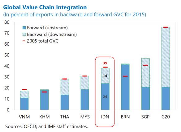
INDONESIA

Indonesia has one of the largest shares in terms of forward GVC linkages, measured by the domestic
value added embodied in foreign exports (as share of gross exports). On the other hand, it also has
a high degree of backward linkages; as of 2016, 14 percent of Indonesian exports have foreign
value-added content. Further, many of the intermediate imports are often used for re-exports. The
share of intermediate goods import used for re-exports is 20 percent, on average in Indonesia.
Exploiting the sectoral variation in backward participation and intensity of re-exports, we find several
interesting effects.11 First, export pass-throughs are very sensitive to the share of foreign
value-added content embodied in the sector’s exports. Sectors with less dependence on imports for
producing exports, i.e., with lower backward linkages are more likely to have high exchange rate
pass-through effects on export prices. The same holds for commodity price effects but the
difference is much smaller. Second, import price pass-throughs also vary by the extent of the share
of imports used for re-exports. Those sectors with high shares of re-exported imports experience
lower price pass-through effects of exchange rate shocks relative to sectors with a smaller share of
imports for re-exportation needs. One reason for such an effect could be that this reflects weak
substitutability between domestic and foreign goods, in the sense that these imports are essential
for exports and limit the extent of expenditure switching.

19. Taken together, the results suggest that while trade prices adjust less than fully to
exchange rate and commodity price shocks, volumes adjust strongly and almost
instantaneously to price changes. Combined, these results indicate that exchange rate fluctuations
can have a significant impact on the current account, by affecting net-exports through trade price
and quantity adjustment. However, we do find incomplete adjustment of trade prices concentrated
in the top import/export sectors over shorter time-horizons. We find that the pass-through effects
vary substantially across sectors and, additionally, that appreciations have stronger pass-through
effects than depreciation, confirming the asymmetries in the effects. We also find suggestive

11 Thisspecification augments the pass-through equations with global value-chain measures of backward
participation (share of imports used for exports) and re-export intensity (share of imports that are re-exported) for
exports and imports respectively. See OECD (2018) and Koopman and others (2014) for details. These measures are
then interacted with the exchange-rate and commodity price change variables.

 INTERNATIONAL MONETARY FUND 13

INDONESIA

evidence that the extent of pass-through is weaker when exchange rate changes derive from
financial market perturbations and when sectors are more tightly connected in the global value-
chain for re-import and re-export purposes.

20. In conclusion, this paper’s analysis weaves together several elements that determine
the transmission of exchange rates fluctuation to trade. It documents frictions in the adjustment
of trade prices to exchange rate shocks that depend on the source of the exchange rate fluctuation
as well as transmission mechanism related to the trade integration in global value chains. These
results obtained in the paper are overall consistent with the existing literature on exchange rate
pass-through effects, where it is found that (i) aggregate pass-through effects of exchange rate
changes on trade prices are incomplete (Campa and Goldberg 2005; Gopinath and Itskhoki, 2010);
(ii) exports that are highly dependent on imports have low sensitivity to exchange rate shocks (Amiti
and others, 2019.), and; (iii) financial sector driven exchange rate shocks are weakly transmitted to
the real economy (Forbes and others, 2019).

14 INTERNATIONAL MONETARY FUND

INDONESIA

 References
Amiti, M., O. Itskhoki, and Konings, J., 2014, “Importers, Exporters, and Exchange Rate
 Disconnect,” American Economic Review, Vol. 104, Issue 7, pp. 1942−78.

Baxter, M., and A.C. Stockman, 1989, “Business Cycles and the Exchange-Rate Regime: Some
 International Evidence,” Journal of monetary Economics, Vol. 23, Issue 3, pp. 377−400.

Bussière, M., Delle Chiaie, S. and Peltonen, T.A., 2014. “Exchange rate pass-through in the global
 economy: the role of emerging market economies”. IMF Economic Review, 62(1), pp.146-178.

Campa, J.M., and L.S. Goldberg, 2005, “Exchange Rate Pass-Through into Import Prices,” Review of
 Economics and Statistics, Vol. 87, Issue 4, pp. 679−690.

Chari, V.V., P.J. Kehoe, and E.R. McGrattan, 2002, “Can Sticky Price Models Generate Volatile and
 Persistent Real Exchange Rates?,” The Review of Economic Studies, Vol. 69, Issue 3,
 pp. 533−563.

Devereux, M.B., and C. Engel, 2002, “Exchange Rate Pass-Through, Exchange Rate Volatility, and
 Exchange Rate Disconnect,” Journal of Monetary economics, Vol. 49, Issue 5, pp. 913−940.

Engel, C., 2002. “Expenditure switching and exchange-rate policy”, NBER macroeconomics annual, 17,
 pp.231−272.

Forbes, K., I. Hjortsoe, and T. Nenova, 2018, “The Shocks Matter: Improving Our Estimates of
 Exchange Rate Pass-Through,” Journal of International Economics, Vol. 114, pp. 255−275.

Gopinath, Gita, and Roberto Rigobon, 2008, "Sticky borders," The Quarterly Journal of Economics,
 Vol. 123, No. 2, pp. 531–575.

––––––––, and O. Itskhoki, and R. Rigobon, 2010, “Currency Choice and Exchange Rate
 Pass-Through,” American Economic Review, Vol. 100, Issue 1, pp. 304−36.

––––––––, and O. Itskhoki, 2010, “Frequency of Price Adjustment and Pass-Through,” The Quarterly
 Journal of Economics, Vol. 125, Issue 2, pp. 675−727.

Imbs, J., and I. Mejean, 2015, “Elasticity Pptimism,” American Economic Journal: Macroeconomics,
 Vol. 7, Issue 3, pp. 43−83.

International Monetary Fund, 2015, “Exchange Rate and Trade Flows: Disconnected?,” Chapter 3 in
 World Economic Outlook, October 2015: Adjusting to Lower Commodity Prices, World
 Economic and Financial Surveys (Washington).

Itskhoki, O., and D. Mukhin, 2017, “Exchange Rate Disconnect in General Equilibrium,” NBER Working
 Paper No. 23401 (Cambridge, Massachusetts: National Bureau of Economic Research).

 INTERNATIONAL MONETARY FUND 15

INDONESIA

Koopman, R., Z. Wang, and S.J. Wei, 2014, “Tracing Value-Added and Double Counting in Gross
 Exports,” American Economic Review, Vol. 104, Issue 2, pp. 459−94.

Krugman, P.R., 1989. Exchange-rate instability, MIT Press, Cambridge, MA.

Obstfeld, M., 2001. “International macroeconomics: beyond the Mundell-Fleming model”, National
 Bureau of Economic Research, No. w8369.

Organisation for Economic Co-operation and Development, 2018, “The Changing Nature of
 International Production: Insights from Trade in Value Added and Related Indicators,” OECD
 TiVA Indicators 2018 Update (Paris).

16 INTERNATIONAL MONETARY FUND

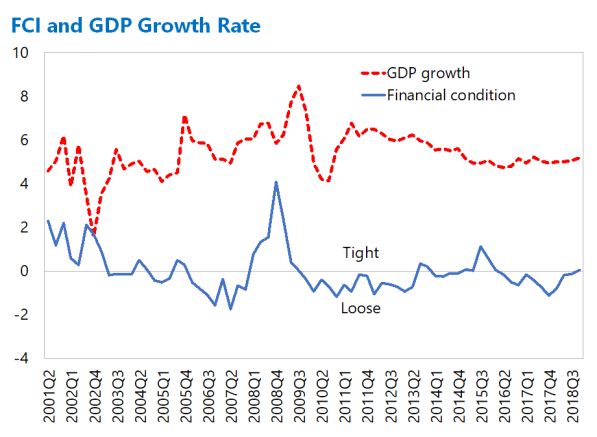
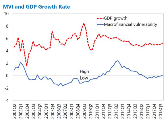
INDONESIA

INDONESIA'S GROWTH-AT-RISK1
Macrofinancial conditions serve as a useful predictor for downside risks to GDP growth (Adrian and
others, 2019). A principal component analysis shows that tighter financial conditions and elevated
macrofinancial vulnerability in Indonesia have been associated with a decline in future GDP growth.
Using a country-specific financial condition Index and a macrofinancial vulnerability index for
Indonesia, the Growth-at-Risk analysis shows that both financial condition and macrofinancial
vulnerability index were at a neutral level at end-2018, and that the 2019 GDP growth rate will be
most likely to be 5.2 percent, conditional on two neutral indices.

1. In a globally integrated financial system, changes in the domestic and global financial
conditions and the evolution of macrofinancial vulnerabilities can provide powerful signals
about risks to future economic activity (Prasad and others, 2019). As in the runup to the global
financial crisis, macrofinancial vulnerabilities often increase in buoyant economic conditions when
funding is widely available and risks appear subdued. Once these macrofinancial vulnerabilities are
sufficiently elevated, a tightening of financial conditions pose significant downside risks to economic
activity over the medium term. Thus, tracking the evolution of financial conditions and
macrofinancial vulnerabilities can provide valuable information for policymakers regarding risks to
future growth and also a basis for targeted preemptive action.

2. The growth-at-risk (GaR) framework links both financial conditions and macrofinancial
vulnerability to the probability distribution of future GDP growth (IMF, 2017; IMF, 2018). The
GaR framework offers a number of appealing features that enhance macrofinancial surveillance,
which has focused on the central forecast. First, it allows to take into consideration the entire growth
distribution—reflecting both downside and upside risks—in addition to the central forecast. Second,
it provides a framework to analyze key driving factors for future real GDP growth, including their
relative importance over different forecasting horizons.2 Third, it helps quantify the impact of
systemic risk on future real GDP growth and the intertemporal tradeoff associated with a tighter
macroprudential stance.3

3. The first step of the GaR analysis is to select relevant macrofinancial variables, group
them into partitions (i.e., groupings), and estimate a level of financial conditions and
macrofinancial vulnerability. Using partitions instead of individual variables, one can extract
common trends among relevant macrofinancial variables and remove idiosyncratic noise, thereby
improving the quality of the subsequent analyses. For Indonesia, the team categorizes
macrofinancial variables into three partitions: (1) financial conditions; (2) macrofinancial vulnerability;
and (3) external factor. Given high exposures of domestic financial sectors to the global financial

1
 Prepared by Heedon Kang (MCM).
2For example, in the near term, loose financial conditions can help support growth. But, over the medium-term, they
can induce a build-up of macrofinancial imbalances that could undermine growth down the road.
3While such a tightening could induce a short-term slowdown, it could lower the medium-term downside risks to
growth with contained macrofinancial vulnerabilities.

 INTERNATIONAL MONETARY FUND 17

INDONESIA

market developments, the first partition captures both the domestic and global price of risk
embedded in asset prices, the cost of funding, and the degree of domestic and global financial
stress. The second partition represents macrofinancial imbalances which develop endogenously and
act as potential amplifiers of negative developments of financial conditions. Lastly, given the role of
China as the main trading partner, its growth is included as the external factor that influences future
growth in Indonesia (Table 1).

 Table 1. Indonesia: List of Macrofinancial Variables for GaR Analysis

Financial conditions • Real long-term interest rates
 • Term spread
 • Sovereign spreads
 • Corporate spreads
 • CEMBI market cap
 • Equity returns
 • Change in foreign exchange rate
 • VIX
Macrofinancial vulnerability • Credit growth
 • Credit gap
 • NPL ratios in the banking system
 • Ratio of external debt to GDP
 • Ratio of currency account balance to GDP
 • House price growth
External condition • China’s GDP growth

4. Financial conditions serve as a useful predictor for downside risks to GDP growth
(Adrian and others, 2019). Using the principal component analysis (PCA), the financial condition
index (FCI) is constructed by extracting the first principal component from a collection of eight
financial variables. As shown Figure 1, the FCI is found to be a good leading indicator of GDP. The
accompanying factor loadings show that both domestic and external financial conditions
(e.g., sovereign spreads and VIX) play an important role in explaining future GDP growth in
Indonesia. The Global Financial Crisis is clearly reflected in the FCI by a sharp tightening, and other
episodes, such as the taper tantrum in 2013 and the global stock market in 2015, are also
noticeable, which reflect well the heavy reliance on capital flows to finance the current account and
fiscal deficits.

5. Financial conditions in Indonesia have tightened to a neutral level at end-2018. This
tightening has been mainly driven by worsening external financial conditions and global trade
tensions, whose developments Indonesia remains exposed to. It was also partly contributed by BI’s
policy rate hikes, which was done as a response to the global market turbulence and the EM sell-off
in 2018. However, financial conditions in Indonesia are still at the neutral level by historical
standards and are expected to loosen a bit in 2019:Q1, based on growing optimism about U.S.-
China trade negotiations and expectations that major central banks would take a more patient

18 INTERNATIONAL MONETARY FUND

INDONESIA

approach to monetary policy normalization. Thus, they would continue to be supportive of growth
in the near term for Indonesia.

6. Macrofinancial vulnerability index (MVI) captures credit boom-bust cycles and
macrofinancial imbalances in the housing market and external sector in Indonesia. The first
principal component from a list of slow-moving credit aggregates and sectoral indicators
summarizes the level of systemic risk in Indonesia. As shown in Figure 2, current account deficits and
credit gap are the two most important variables to explain the level of macrofinancial vulnerability in
Indonesia.

7. As of end-2018, macrofinancial vulnerability is broadly contained. Indonesia’s external
debt is still moderate and sustainable. The credit cycle moved out of a prolonged downturn with
credit gap closing, and the banking system remains broadly sound with large capital buffers, strong
profitability, and asset quality improvement. However, the vulnerability level turned to slight positive
as current account deficits were widened and corporate external debt increased.4 It can be elevated
further if credit, especially to the corporate sector, grows rapidly without reins.

8. In general, tighter financial conditions and elevated macrofinancial vulnerability are
associated with a decline in future GDP growth (Figure 3). Quantile regressions, which estimate
relationships between selected explanatory variables (e.g., financial conditions, macrofinancial
vulnerability partition) and quantiles of future GDP growth rates, find that the relationships vary over
the forecasting horizon and differ across quantiles in Indonesia. Tight financial conditions are
negatively correlated with economic activities in the near term. However, as financial conditions
revert to their historical average, they tend to boost growth over the medium term. In contrast,
when macrofinancial vulnerability is elevated, risks to future GDP growth is also high not only in the
near term but also over the medium term.

9. Given the neutral financial conditions and macrofinancial vulnerability, the 2019 GDP
growth rate is most likely to be 5.2 percent under the baseline (Figure 4). The distribution of
4-quarter ahead GDP growth is derived by fitting a t-skew distribution to predicted values of the
conditional quantile regressions. The predicted growth mode for one-year ahead closely tracks the
realized growth, especially since the global financial crisis (the bottom left chart). The GaR at
5 percent is 2.7 percent, implying that there is a 5 percent chance that real GDP in 2019 will grow by
at most 2.7 percent. The probability of a recession is less than 1 percent in 2019 (the bottom right
chart). The interquartile interval of the GDP forecast ranges from 3.9 to 5.3 percent at the end
of 2019, with the mode and median being 5.2 and 4.5 percent.

4 Current account deficits are expected to gradually narrow over the medium term.

 INTERNATIONAL MONETARY FUND 19

INDONESIA

 Figure 1. Indonesia: Financial Condition Index 1/

Source: IMF staff estimates.
1/ The FCI is normalized to have zero mean and a standard deviation of one over 2001–2018.

 Figure 2. Indonesia: Macrofinancial Vulnerability Index 1/

Source: IMF staff estimates.
1/ The MVI is normalized to have zero mean and a standard deviation of one over 2001–2018.

20 INTERNATIONAL MONETARY FUND

INDONESIA

 Figure 3. Indonesia: Quantile Regression Results
Tighter financial conditions are associated with lower GDP growth in the next year, when economic activity is weak, while
they are associated with stronger GDP growth over the medium term.
 Quantile Regression Coefficient for Financial Conditions over 4-, 8-, and 12-Quarters Ahead

Elevated Macrofinancial vulnerability is associated with weaker growth regardless of the horizon, but the impact of potential
shock amplification is larger over the medium term.
 Quantile Regression Coefficient for Macrofinancial Vulnerability over 4-, 8-, and 12-Quarters Ahead

Source: IMF staff estimates.

 Figure 4. Indonesia: Growth-at-Risk Results

Source: IMF staff estimates.

 INTERNATIONAL MONETARY FUND 21

INDONESIA

 Appendix I. Data Source

 Variables Description Source

 Change in Long-Term Real Percentage point change in the 10-year Bloomberg Finance L.P.; IMF staff
 Interest Rate government bond yield, adjusted for estimates
 inflation
 Term Spreads Yield on 10-year government bonds Bloomberg Finance L.P.; IMF staff
 minus yield on 1-year government estimates
 bonds
 Sovereign Spreads Yield on 10-year Indonesia government Bloomberg Finance L.P.; IMF staff
 bonds minus yield on 10-year estimates
 U.S. government bonds
 Corporate Spreads Commercial banks’ lending rates for CEIC data Co.; IMF staff estimates
 corporate working capital minus
 interbank interest rate
 CEMBI market cap Market capitalization of Indonesia Bloomberg Finance L.P.
 corporate debt securities in CEMBI
 Equity Returns (local Log difference of the Jakarta stock Bloomberg Finance L.P.
 currency) market index
 Exchange Rate Movements Change in U.S. dollar per national Bloomberg Finance L.P.; IMF staff
 currency exchange rate. estimates.
 CBOE Volatility Index (VIX) A measure of expected price fluctuations Bloomberg Finance L.P.
 in the S&P 500 Index options over the
 next 30 days
 Credit Growth Year-on-year growth rate of loans to CEIC data Co.; IMF staff estimates
 private sectors
 Credit Gap the difference between the credit-to- CEIC data Co.; IMF staff estimates
 GDP ratio and its long-term trend, which
 is estimated with one-sided HP filter
 NPL Ratio Ratio of nonperforming loans to total Haver Analytics; IMF staff estimates
 loans in the banking system
 External Debt to GDP Ratio of external debts to GDP Haver Analytics; IMF staff estimates

 Currency Account Deficits Ratio of current account deficits to GDP Haver Analytics; IMF staff estimates
 (relative to GDP)

 House Price growth Year-on-year growth rate of residential Haver Analytics; IMF staff estimates
 property price index
 Real GDP Growth for Percent change in GDP at constant prices IMF, World Economic Outlook
 Indonesia for Indonesia database
 Real GDP Growth for China Percent change in GDP at constant prices IMF, World Economic Outlook
 for China database

22 INTERNATIONAL MONETARY FUND

INDONESIA

Appendix II. Parametric Estimation of Future Growth Distribution
Estimation of the Conditional Quantiles

For a set of horizons ℎ ∈ {4, 8, 12} where h represents the quarters ahead, the following
specifications are estimated:

 +ℎ = + ∑ , + , 
 
 ∈ 
Where +ℎ represents future GDP growth h quarters ahead, , is the partition i (financial condition,
macrofinancial vulnerability, and external factor), the coefficient of the quantile regression,
 the associated constant and , 
 
 the residual. The quantile regressions are estimated at different
points of the distribution of +ℎ , ∈ {10, 25, 50, 75, 90}. A quantile regression at the 10th percentile
would estimate a relationship when GDP growth is relatively weak, while a quantile regression at the
90th percentile would show one when growth is strong. Using quantile regressions for estimating the
conditional distribution has many advantages: first, under standard assumptions, quantile
regressions provides the best unbiased linear estimator for the conditional quantile; second,
quantile regressions are robust to outliers. Finally, the asymptotic properties of the quantile
regression estimator are well-known and easy to derive.

Parametric Fit of the Conditional Distribution of Future GDP Growth

The conditional quantiles are sufficient statistics for describing the full conditional cumulative
distribution function (CDF). From the CDF, we derive the probability distribution function using a
parametric method to fit the conditional quantiles for the sake of robustness with regards to
quantiles crossing and extreme quantiles estimation. Following Adrian and others (2016), a
parametric t-skew fit is used to represent more accurately fatter tails. The skew version of the t-
distribution is useful to model tail events, given that most of the macro-financial variables present
this feature.

Fitting the CDF estimated from the quantile regressions represents another robust dimensionality
reduction, after the data partitioning presented above. The Student t-skew distribution is fully
characterized by five parameters (location/mode, degree of freedom, scale/variance, kurtosis, and
skewness) which represents a good compromise between describing the distribution as accurately
as possible and keeping a low number of parameters to avoid over-fitting.

The estimation of the t-skew distribution parameters is done in two different steps. First, degrees of
freedom are computed directly while the mean parameter of the conditional distribution can be
retrieved from OLS fit, with the same specification as the quantile regressions:

 ∗ = ( [ +ℎ |{ } ∈ ]) = ( ̂ + ∑ ̂ , )
 ∈ 
Second, the sigma, the kurtosis, and the skewness, which are truly the quantities of interest, are
estimated via the following minimization program:

 INTERNATIONAL MONETARY FUND 23

INDONESIA

 sigma∗ , skew ∗ , kurtosis ∗
 = [ ∑[ . ( , ∗ , ∗ , , , )
 − ( +ℎ , | { } ∈ )]2 ]

Once the optimal three t-skew parameters have been estimated from the conditional quantiles, it is
straightforward to derive the fitted t-skew cdf and pdf, therefore allowing to estimate the associated
Growth-at-Risk.

24 INTERNATIONAL MONETARY FUND

INDONESIA

 References
Adrian, Tobias, Nina Boyarchenko, and Domenico Giannone, 2019, “Vulnerable Growth,” American
 Economic Review, Vol. 109, No. 4, April.

International Monetary Fund, 2017, “Financial Conditions and Growth at Risk,” Chapter 3 in Global
 Financial Stability Report October 2017, (Washington).

–––––––, 2018, Singapore—Staff Report for the 2018 Article IV Consultation (Washington).

Prasad, Ananthakrishnan, Selim Elekdag, Phakawa Jeasakul, Romain Lafarguette, Adrian Alter, Alan
 Xiaochen Feng, and Changchun Wang, 2019, “Growth at Risk: Concept and Application in
 IMF Country Surveillance,” IMF Working Paper No. 19/36 (Washington: International
 Monetary Fund).

 INTERNATIONAL MONETARY FUND 25

INDONESIA

IMPACT OF MONETARY POLICY COMMUNICATION IN
INDONESIA1
This paper assesses the impact of monetary policy communication in Indonesia, focusing on the
features and impact of monetary policy press releases and reports. It shows that the transparency of
monetary policy has improved significantly over time, as monetary policy press releases have provided
more information. However, the clarity of the messages appears to have declined. The paper also
highlights that surprises on monetary policy decisions are relatively frequent, though the size of the
surprises is small. Press releases and monetary policy reports do not appear to have a significant
impact on market rates.

1. Communication is an important tool of monetary policy at Bank Indonesia (BI). With
the adoption of an inflation targeting framework in 2005, transparency and clarity of monetary
policy has played an increasingly important role in guiding market expectations. As a result,
communication tools and events have increased over time. BI has increased its disclosure of
information relevant for monetary policy through press releases, monetary policy reports, monetary
policy reviews, speeches by senior BI officials, press conferences, and outreach.

2. This paper assesses the impact of monetary policy communication in Indonesia from
three perspectives. First, the transparency and clarity of monetary policy communication is key to
align BI and the market’s understanding of the drivers of monetary policy decisions. Second, with
this alignment in understanding, monetary policy decisions should be generally predictable for the
market. Third, the efficacy of monetary policy can be strengthened with communication with the
latter clarifying policy decisions, or providing new information not previously priced in market rates.

3. The analysis presented below focuses on two tools of monetary policy communication
at BI—monetary policy press releases and monetary policy reports. Press releases are issued at
the end of the regular monthly or extraordinary monetary policy committee meetings. Monetary
reports are published on a quarterly basis. For other months of the year, BI issues monetary policy
reviews, which are similar to the monetary policy reports, excluding the forward-looking analysis. In
this paper, references to monetary policy reports encompass both monetary policy reports and
reviews. The reports are not issued on the same day as the monetary policy press release, allowing a
separated identification of their impact.

A. Transparency and Clarity

4. Transparency of monetary policy has improved over time. Transparency is a key element
of accountability and a way to enabling markets to respond more smoothly to policy decisions.
Transparency provides the public with a better understanding of the central bank’s objective and the
factors that motivate monetary policy decisions (Dincer and Eichengreen, 2014). The Dincer-

1 Prepared by C. Ahokpossi, A. Isnawangsih, S. Naoaj (all APD), and T. Yan (COM). K. Moriya and T. Wanasukaphun
(both ITD) assisted with the textual analysis.

26 INTERNATIONAL MONETARY FUND