INVESTIGATING GENDER STEREOTYPES IN THE MEDIA: DIVA
←
→
Page content transcription
If your browser does not render page correctly, please read the page content below
Linköping University | Department of Management and Engineering
                                               Master’s thesis, 30 credits| Master’s programme
                                                      Spring 2021| LIU-IEI-FIL-A--21/03695--SE

Investigating gender
stereotypes in the media:
A Natural Language Processing approach to understanding
gender disparities in the reporting of football.

Isabel Pereira Fernandez

Supervisor: Miriam Hurtado Bodell
Examiner: Erik Rosenqvist

                                                                          Linköping University
                                                                 SE-581 83 Linköping, Sweden
                                                                 +46 013 28 10 00, www.liu.se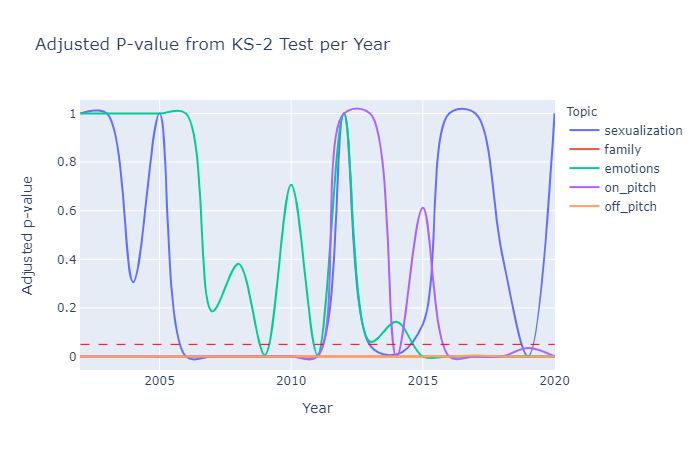
Contents

1 Introduction                                                                         1

2 Literature Review                                                                    3

  2.1   Gender Stereotypes . . . . . . . . . . . . . . . . . . . . . . . . . . . .     3

  2.2   Media’s role in gender stereotypes . . . . . . . . . . . . . . . . . . . .     4

        2.2.1   Semantic Differences . . . . . . . . . . . . . . . . . . . . . . .     4

        2.2.2   Syntactical Differences . . . . . . . . . . . . . . . . . . . . . .    6

  2.3   History of Women’s Football in the UK . . . . . . . . . . . . . . . . .        8

3 Data & Methods                                                                      10

  3.1   Data . . . . . . . . . . . . . . . . . . . . . . . . . . . . . . . . . . . . 10

  3.2   Seeded Topic Modelling . . . . . . . . . . . . . . . . . . . . . . . . . 12

        3.2.1   Jensen–Shannon Divergence . . . . . . . . . . . . . . . . . . . 14

        3.2.2   Two Sample Kolmogorov–Smirnov Test . . . . . . . . . . . . . 15

  3.3   POS Tagging . . . . . . . . . . . . . . . . . . . . . . . . . . . . . . . 16

        3.3.1   Mann–Whitney U test . . . . . . . . . . . . . . . . . . . . . . 17

        3.3.2   Top Word Analysis . . . . . . . . . . . . . . . . . . . . . . . . 18

  3.4   Bonferroni Correction . . . . . . . . . . . . . . . . . . . . . . . . . . . 19

4 Results                                                                             20

  4.1   Semantic Gender Differences . . . . . . . . . . . . . . . . . . . . . . . 20

  4.2   Syntactic Gender Differences . . . . . . . . . . . . . . . . . . . . . . . 25

5 Discussion                                                                          33
6 Conclusion 35 A List of Words Used for Categorization 37 B List of Seed Words Used 37 C Seeded Topic Models Robustness Test 38 D Full list of topics and top words 42 E Keyword Robustness Test 49 E.1 POS Tag Results . . . . . . . . . . . . . . . . . . . . . . . . . . . . . 50 E.2 Seeded Topic Model Results . . . . . . . . . . . . . . . . . . . . . . . 57 References 60
List of Figures

  1   Number of Articles in the Dataset Over the Years . . . . . . . . . . . 11

  2   Intuition behind LDA model from Blei (2012) . . . . . . . . . . . . . 12

  3   How to Calculate the Two Sample Kolmogorov–Smirnov Test Statistic 16

  4   Jensen–Shannon Divergence For Each Topic For Different Sized Bins        22

  5   Average Jensen–Shannon Divergence For Each Topic Over Time . . . 24

  6   Adjusted P-values for the Two Sample Kolmogorov–Smirnov Test per
      Topic Over Time . . . . . . . . . . . . . . . . . . . . . . . . . . . . . 24

  7   Overview of results for the POS tag analysis on nouns and pronouns . 29

  8   Overview of results for the POS tag analysis on adjectives and adverbs 30

  9   Overview of results for the POS tag analysis on verbs . . . . . . . . . 31

List of Tables

  1   Most Common Topics For Men’s Football Articles . . . . . . . . . . . 21

  2   Most Common Topics For Women’s Football Articles . . . . . . . . . 21

  3   Results for the Two Sample Kolmogorov–Smirnov Test . . . . . . . . 23

  4   Results for Mann–Whitney U test on POS tag ratios . . . . . . . . . 25

  5   Most Common Unique Words in Category For Each Tag . . . . . . . 27

  6   Percentage of Words in the Top 500 That Are Different For Each Tag 28
Abstract
Sports can be an important factor in defining gender identity. However,
sports are generally perceived as a masculine activity, especially when they
are highly physical. In turn, this negatively impacts women who want to par-
take in such activities. The most widely watched sport that is perceived to be
masculine is football, it reaches billions of people across the world. Since the
media is the main source of information for thousands of people who follow
football, it is important to understand what part the media play in reproduc-
ing gender stereotypes. The aim of this research is to investigate this phe-
nomenon by answering the following research question: In what ways does the
media reproduce gender stereotypes when reporting on football?. To do that,
all articles from the Football section of the British newspaper The Guardian
published between 2002 and 2020 were collected. The analysis is divided into
two parts: semantic and syntactical differences. First, a seeded topic model is
used to investigate whether the media focuses on different aspects of the sport
depending on what gender they reported on. Second, a POS tag analysis is
conducted to examine if the media employs different syntax on the coverage of
men’s and women’s football. This is the first large-scale longitudinal study to
examine gender differences in the media reporting in sports as well as one of
few to use machine learning to analyse gender stereotypes. Findings indicate
that both semantic and syntactical differences are prevalent in the reporting.
More specifically, results demonstrate that there is a greater focus on female
footballers’ personal life, whereas for male football players the spotlight is
on their performances and accomplishments on the pitch. Furthermore, the
syntactical analysis indicates that the media uses gendered language more of-
ten when reporting on women’s football, and utilizes action-packed language
when covering men’s football. In both semantic and syntactic aspects, the
longitudinal analysis demonstrates that the differences are diminishing over
time.1 Introduction
Sports are an important factor in defining gender identities and stereotypes (Thorpe,
2010). From an early age, sports are seen as a male activity, especially when
they require masculine attributes such as physical strength, violence and risk-taking
(Musto, Cooky, & Messner, 2017; Thorpe, 2010). Therefore, women have a tendency
to participate in physical activities that are classified as woman-like and avoid those
that are perceived as more masculine. In England, for example, 67% of adult men
practice sports regularly, compared to 55% of women (World Health Organization,
2015). This suggests that men are indeed more inclined to practice sports.
Football makes for a ideal candidate to study gender stereotypes in sports due
to its vast popularity and as it is perceived as a masculine activity. Football is a
contact sport which requires strength and aggression (Harris, 2005), and is there-
fore regarded as an activity more suited for men, stigmatizing women’s football. In
terms of the number of players, in England, the gap is even larger than that of ac-
tive adults mentioned above: only 24% of registered footballers are women, with the
remainder 76% being men (The Football Association, 2015). In general, women’s
football is less popular than men’s. However, over the last decades, women’s football
has received increased attention and gained popularity. The Women’s World Cup
for example, had a growth of 65% in viewership from 2015 to 2019, reaching over 1.2
billion viewers (FIFA.com, 2019). Despite the increase in popularity, it is still only
a fraction of the viewership of the men’s events. In 2018, the men’s World Cup final
alone amounted to the same number of views as the whole women’s tournament in
2019. In fact, the men’s version of the tournament in its entirety received over 3.5
billion views, matching the Olympic Games in terms of viewership (FIFA, 2018).
This is especially impressive since the Olympic Games are the most important sport-
ing event to take place, as it includes more than 30 different sports with participants
from over 200 countries (Whannel, 1992). Put together, these characteristics make
for an interesting case-study, as football is a male-typed activity with large following
which has undergone a change in the gender composition within the sport in recent
years.
Media outlets have an important role in influencing gender stereotypes and gen-
der roles. This is because they can frame a story as they wish, and since they
have a large reach, they can influence those who receive the story through their
lens (Altheide & Snow, 1992; Rogers, 2004). In other words, the way in which a
piece portrays a person impacts how the readers of said piece will perceive them.
It has been shown that articles covering male and female athletes tend to use dif-
ferent language and focus on different aspects of their performance (Eastman &
Billings, 2000; Messner, Duncan, & Jensen, 1993; Musto et al., 2017; Wensing &
1Bruce, 2003). This can lead people to perceive men and women in sports differently.
Therefore, it is important to understand how the media portrays male and female
athletes. Based on that, the following research question arises:
In what ways does the media reproduce gender stereotypes when reporting on
football?
As mentioned above, previous literature has found that gender stereotypes are
reproduced by the media both through the topics covered and the language used.
In that sense, both semantics and syntax play a role in the differential coverage
between men’s and women’s football. As a result, two sub questions are formulated:
What are the semantic differences on the reporting of male and female footballers
and do they change over time?
To what extent does the syntax used by the media lead to different portrayal of
men and women in football and how does it evolve over time?
To answer these questions, data from the British newspaper The Guardian is
used. The dataset consists of all articles about football published by the newspaper
from 2002 to 2020. These articles are categorized by the gender they refer to using
keywords. Once the data has been appropriately categorized, two machine learning
techniques are used to obtain results. First, a seeded topic model is adopted to
examine the data semantically. Second, part-of-speech (POS) tagging is applied to
study the syntactical content of the data.
The present study expands on previous literature in two ways. First, it examines
a period of 19 years of coverage without any interruption, something that has not yet
been done. This enables for a longitudinal investigation of how gender stereotypes
in football evolve over the years. Second, it makes use of machine learning, which
previously has not been used to study gender differences in sports. This approach
also allows for a larger volume of data to be analyzed.
This paper will continue as follows: first, a literature review will outline previous
studies in the field and, based on that, draw six hypothesis which will be investigated.
Then, the data and methods will be described in more detail. After this, results are
presented and interpreted, followed by a discussion of the findings and the potential
shortcomings of this analysis.
22 Literature Review
2.1 Gender Stereotypes
Stereotypes were first defined by Lippmann (1922), who described it as illogical
generalizations about social groups that are erroneous, that is, incorrect. Since
then, studies have demonstrated that this is not necessarily the case, stereotypes
can, in fact, be accurate (Judd & Park, 1993; Jussim, 1991). Therefore, stereo-
types are defined as generalizations of characteristics, attributes, or behaviours of
members of a given group (Hilton & Von Hippel, 1996). Stereotypes can be explicit
or implicit. Implicit stereotypes are beliefs about a group that are unconsciously
activated, whereas explicit stereotypes are a set of beliefs that a person consciously
associates with a given group (Greenwald & Banaji, 1995).
Gender is one of the most prominent features in a person when it comes to
categorization and perception (Ito & Urland, 2003; Ellemers, 2018). To put it
differently, when a person is surrounded by strangers, gender is one of the main
attributes that will be used to categorize these people and obtain a first impression.
The inferences that are made when this categorization happens stem from gender
stereotypes. In the case of gender, these assumptions are made based on how men
and women are expected to behave. Gender creates such prominent stereotypes that
children at the age of 6 already display awareness of their existence (Bian, Leslie, &
Cimpian, 2017).
Although some believe that gender differences stem from biological factors, this
has been proven to not be the case. Joel et al. (2015) find that there are no clear
differences between female and male brains that create such a distinguishable dif-
ferentiation as with gender expression. Moreover, a body of research demonstrates
that there are no, or very small gender differences when it comes to mathematics
and verbal skills (Lindberg, Hyde, Petersen, & Linn, 2010; Else-Quest, Hyde, &
Linn, 2010; Hyde & Linn, 1988; Leaper & Robnett, 2011), as well as leadership
ability (Eagly & Carli, 2003) and displaying of emotions (Chaplin & Aldao, 2013;
Else-Quest, Higgins, Allison, & Morton, 2012). Instead, research shows that gender
and gender stereotypes are constructed over time, through socialization processes
(West & Zimmerman, 1987; Lorber, 1994; Bem, 1981).
Research has also demonstrated that gender stereotypes have negative effects
both on men and women. Bian et al. (2017) find that young girls are less likely
than young boys to think other children of the same gender are smart, causing them
to avoid activities they perceive as intelligent. This has significant effects on their
life outcomes: women are less likely to follow a career in science fields and those
3who do are perceived as less talented by both men and women (Leslie, Cimpian,
Meyer, & Freeland, 2015). In fact, gender stereotypes negatively affect women’s
careers in general: Heilman (2012) shows that gender stereotypes lead to penalties
for women in the workplace, as their characteristics and skills are perceived as a poor
match for leadership positions. On top of that, these gender differences that stem
from stereotypes create a gender wage gap (Angelov, Johansson, & Lindahl, 2016;
Bertrand, Goldin, & Katz, 2010; Blau & Kahn, 2017). On the other hand, men
experience more pressure to conform to gender roles and prove their masculinity by
being strong, self-reliant and not displaying weakness (Prentice & Carranza, 2002;
Vandello & Bosson, 2013). As a consequence, men are more likely than women to
take risks (e.g: smoking, horse-riding, rock climbing), in order to affirm their gender
identity (Byrnes, Miller, & Schafer, 1999).
2.2 Media’s role in gender stereotypes
There are two ways in which the media reproduces gender stereotypes. Firstly, the
choice of topics to be covered by the media, the emphasis that is placed on them and
how they are framed can reinforce existing stereotypes. Second, the choice of words
used to report on an event, beside the topical context, can also have the potential
to replicate stereotypes.
2.2.1 Semantic Differences
Mass media has the ability to tell a narrative to millions of people, and therefore
affect how they perceive a certain story, subject or individual. For this reason, the
way in which they choose to frame a given situation can impact how people view
it. Framing can be defined as the “conceptual tools which media and individuals
rely on to convey, interpret and evaluate information” (Neuman, Just, & Crigler,
1992, p. 60). To put it differently, framing refers to how individuals or groups give
meaning to an issue or situation (Entman, 1993; Goffman, 1974; Rogers, 2004). In
the case of the media, framing has the power to change the way in which readers
perceive said issue or situation. It has been shown that, in politics, reporters use
different framing based on the gender of the candidate they are reporting on, where
similar activities led to slightly different portrayals for male and female candidates
(Bystrom, Robertson, & Banwart, 2001; Carlin & Winfrey, 2009; Devitt, 2002;
Gidengil & Everitt, 2003; Kittilson & Fridkin, 2008). Moreover, when it comes to
sports, it has been demonstrated that the framing of events shown on television
influence how viewers perceive it (Altheide & Snow, 1992). It is therefore clear
that attention should be paid to how the media chooses to frame female and male
4athletes, as this likely has an impact on how society perceives them and due to the
fact that gender has been shown to be relevant when it comes to framing in other
areas.
An extensive body of literature has demonstrated that there are large differences
between the content of the reporting on male and female athletes. There is a greater
focus on the physical appearance of women than that of men, meaning articles
disproportionately comment on the physique and image of women when compared
to men (Kim & Sagas, 2014; Messner, Duncan, & Cooky, 2003). It has also been
found that news sources make greater use of pictures when they report on women’s
sports (Eastman & Billings, 2000; Sainz-de Baranda, Adá-Lameiras, & Blanco-Ruiz,
2020). This suggests that they use photos to get the readers’ attention, shifting the
spotlight away from female athlete’s sporting ability and achievements, and placing
it instead in their appearance. This is detrimental to female athletes’ image, as it
removes the focus from their athletic ability and changes it to their body image
instead, removing their athlete status. Research shows that sexualized images of
female athletes generates a larger focus on their physical appearance and leads to
them being perceived in a similar way to models, stripping them of their sporting
abilities (Daniels, 2009; Daniels & Wartena, 2011).
Another difference is the depiction of female athletes as woman first, athlete
second. More specifically, when referring to women, the media has a greater focus on
non-sport related aspects of the athlete’s life than when reporting on men. Non-sport
related aspects range from family and dating life to fashion preferences and travelling
(Eastman & Billings, 2000; Messner et al., 1993, 2003; Wensing & Bruce, 2003).
Similar to sexualization, this behaviour draws the focus away from the performance
of women in sports, concentrating instead on their personal lives. This could make
readers give less importance to the ability of female athletes as sportswomen and
instead become interested in them as people, which is diminishing to their career.
Differential framing by the media has also been recognized when describing fail-
ure. When female athletes fail, there are two main reasons that are used to explain
their failure: their lack of commitment, with athletes described as not wanting to
win or not trying hard enough to do so (Angelini, MacArthur, & Billings, 2012;
Eastman & Billings, 2000; Messner, Duncan, & Wachs, 1996); and emotional diffi-
culties, such as lack of confidence (Duncan & Hasbrook, 1988; Messner et al., 1996).
On the other hand, when it comes to reporting on male athletes’ failures, the focus is
different. Research finds that in this case the media attributes losses and mistakes to
the lack of athletic skills of a player (Eastman & Billings, 2000), the elevated quality
of their opponent (Angelini et al., 2012; Messner et al., 1996) or to external factors
such as bad luck (Duncan & Hasbrook, 1988). Overall, despite some variations in
the findings, there are clear differences in the reporting of the media when it comes
5to why athletes fail.
Put together, these discrepancies suggest that the media tends to focus on male
athletes and their achievements within their sports, whereas with women there is a
greater focus on their personal life, their physical appearance and their emotional
state. This leads to the first hypothesis:
H1: Topic distributions of male and female articles will be different
2.2.2 Syntactical Differences
Another way gender stereotypes are reproduced is through language. Lewis and
Lupyan (2020) demonstrate that gender stereotypes arise, in part, from gendered
language. Gendered language entails gender-specific titles (e.g.: ‘Mr.’,‘Miss.’), pro-
nouns, job titles (e.g.: ‘host’, ‘hostess’; ‘actor’, ‘actress’) and other words and phrases
that identify the gender of a subject. Moreover, Garg et al. (2018) investigate word
embeddings over time and how they compare to demographic data from the US
over the same time period. Their results demonstrate that occupational biases
and adjective associations highly correlate with the demographic data. Similarly,
Charlesworth et al. (2021) use word embeddings on a variety of corpora, totalling
over 65 million words, and find that stereotypical personality traits and occupa-
tions can be identified across all their corpora. Put together, results suggests that
syntactical structure has the ability to convey gender stereotypes in an implicit way.
When it comes to sport, research has indicated that there are gender differences
in the language used for the reporting. First of all, the media makes use of gender
marking only when reporting on women’s sports (Higgs, Weiller, & Martin, 2003;
Messner et al., 1993). In other words, the media specifies the gender of the athletes
only when they are women. This establishes men as the standard and suggests that
female athletes and women’s sports are of inferior quality (Messner et al., 1993). A
clear example of this is the official name given by the International Federation of
Association Football (FIFA) to the main competition they organize, the World Cup.
The men’s tournament is simply referred to as the World Cup, whereas the women’s
version is officially called the Women’s World Cup (FIFA, 2021b, 2021a). Moreover,
it has also been found that the media often refers to female athletes by their first
name, however, the norm in sports and the practice with their male counterparts is
to address them by their last name (Fink, 2015; Messner et al., 1993). When female
athletes are not called by their name they are often referred to in general terms
such as ‘ladies’ and ‘little girls’, but that is not the case for the men, who are given
6nicknames (Eastman & Billings, 2000; Wensing & Bruce, 2003). This is the case
both for individuals (e.g.: Ronaldo Nazário is dubbed The Phenomenon; Messi is
called ‘La Pulga’) and teams (e.g.: the Dutch national team is known as the Flying
Dutch Men, Liverpool F.C. is often referred to as The Reds). Put together, research
suggests that the language used by the media when reporting on women’s football
is more gendered than when reporting on men’s football. Therefore, it is expected
that more nouns and pronouns are used when reporting on the women’s game, as
that would reflect gendered language. This leads to hypothesis 2a:
H2a: Articles on women’s football will have a higher ratio of nouns and pronouns
to other POS tags.
Despite the way in which sports people are referred to, the media also uses dif-
ferent syntax when reporting of male and female athletes. Eastman and Billings
(2000) have found that less neutral and factual language, such as ‘dribbling past’
and ‘taking a shot’, is used when reporting on men’s sports. This gives room instead
to adjectival descriptors, for example ‘impressive dribbling’ or ‘powerful shot’. More
specifically, the achievements of men are reported in a descriptive manner, whereas
those of women are recounted in a factual manner. In other words, the accomplish-
ments of women tend to be depicted in an objective manner, their actions are stated
as facts, without descriptive language, such as adjectives and adverbs, to embellish
it. As for men, that is not the case, their performances are illustrated in more detail,
with descriptors that better situate and communicate their accomplishments. One
example of this can be observed when reading the play-by-play reporting of the most
recent World Cup finals, both of which had a penalty in a moment the match was
tied. In the men’s World Cup of 2018, the moment was reported as follows:
‘GOAL! France 2-1 Croatia (Griezmann 38pen) Antoine Griezmann
nonchalantly rolls the ball past Danijel Subasic into the bottom left-hand corner
and France re-take the lead. It’s the World Cup final and it’s 2-1 to the French.’
(Guardian, 2018)
In 2019, during the Women’s World Cup, a very similar moment was reported
in the following manner:
’GOAL: USA 1-0 Netherlands (Rapinoe 61) Struck well as always.’
(Guardian, 2019b)
7These updates report on essentially the same situation, however, it is clear that
Griezmann’s penalty kick was described in more detail. Rapinoe’s shot had only one
descriptive, showing that the reporting was more factual; a goal was scored, but no
further information on it is provided. In terms of syntax, this suggests that articles
about male footballers have more adjectives and adverbs, as those are what makes
language descriptive. This expressed in the following hypothesis:
H2b: Articles on men’s football will have a higher ratio of adjectives and adverbs
to other POS tags.
Similarly, a study by Musto et al. (2017), which analyses four sport shows that
are broadcast in Los Angeles over a period of nine weeks, finds that there is greater
use of action verbs when referring to men than to women. Examples of action verbs
are ‘nailed’, ‘smoked’ and ‘exploded’. Moreover, the language used to describe
male athletes and their achievements is dominant and agentic, suggesting they are
in control of their own destiny, but that is not the case when it comes to female
athletes. For instance, while men are described ‘to be in complete control’ and to
put their opponents ‘in the spin cycle’, women are depicted as ‘having made 27
saves’ or to ‘have put in the work’ (Musto et al., 2017). In fact, this can be seen also
in the example above, with the description of a penalty taken in a World Cup final.
As seen above, Griezmann is depicted to be in control of the situation, by rolling
the ball past the goalkeeper and retaking the lead. On the other hand, Rapinoe is
described to simply strike the ball, with non-agentic language used to explain how
her goal came about. Due to the above mentioned findings, it is expected that the
language used by the media to describe male footballers will have more verbs, as it
is action packed and agentic. Thus, hypothesis 2c is defined as:
H2c: Articles on men’s football will have a higher ratio of verbs to other POS
tags.
2.3 History of Women’s Football in the UK
When studying the media’s reproduction of gender stereotypes in football, it is nec-
essary to consider the history of women’s football. In the UK, there are records of
women playing organized football as early as 1895 (Dunn, 1961; Williams & Wood-
house, 1991). Women’s football became particularly popular during the First World
War, as women got together at work and created teams, and reached its pinnacle
8in December 1920, when over 50, 000 fans gathered to watch a match (Pfister et al.,
2002). Due to its growing popularity, the Football Association (FA) became wor-
ried about the decreased focus on the male teams (Williams & Woodhouse, 1991;
Williams, 2003), and decided to ban women from playing football under questionable
pretenses about how teams were handling money (Pfister et al., 2002; Theivam &
Kassouf, 2019). The ban was made in 1921, and was only lifted in 1971, but women’s
football was not incorporated into the FA until 1993. These factors rendered women
in football invisible for over 50 years, and created a stigma around women who chose
to play, making the women’s game very unpopular (Black & Fielding-Lloyd, 2019;
Meân, 2001).
After being incorporated into the FA, women’s football grew and by 2002 it had
become the most practiced sport amongst girls and women in the UK. Despite an
increase in women playing football, it was only in 2008 that a semi-professional
league was created, with 8 teams competing. The league was very successful and
therefore was expanded over the years, by 2014 it had developed into a two division
competition with 24 teams in total (The Football Association, 2021). It is clear
that women’s football has come a long way since its ban was lifted in 1971 and it is
expected that the reporting on it has also changed.
On top of changes in participation, changes in reporting have also been observed
over the years. Musto et al. (2017) have shown that over time, there was a consid-
erable decrease in explicit sexism observed in the media when reporting on sports.
Similarly, Bruce (2015) demonstrated that there is less use of gender marking in
recent years, and that there has been a shift in the frames used by the media to
report on women’s sports. This suggests that the way in which the media reports
might have changed over time.
Due to increased coverage and participation over the years as well as traces of
change in the reporting of women’s football, it is expected that the media will be
less biased as time goes by. Thus, hypothesis 3 and 4 are defined as follows:
H3: Topic distributions of male and female articles will converge over time
H4: Differences in syntactical aspects between genders will reduce over time.
93 Data & Methods
3.1 Data
Data from the British newspaper The Guardian will be used to carry out the in-
vestigation. The Guardian is one of the most read papers in the UK, it has a
monthly readership of over 24 million, this accounts for consumers of the print ver-
sion, which comes out every day, as well as those who read their articles online
(PAMCo, 2020). On their website, The Guardian claims to not follow any politi-
cal ideology (Guardian, 2015). However, they are known by the public to be left
leaning (Smith, 2017), and even their editors have admitted that the newspaper is
centre-left (Guardian, 2004). Regardless of their political inclination, the newspaper
is considered the most trustworthy in the country (PAMCo, 2020). Furthermore,
The Guardian also has an API which allows for the collection of their articles easily
and for free (Guardian, 2019a).
The Guardian’s API allows for the retrieval of data from their database through
keywords and sections. In this case, searching with keywords could limit the scope
of articles retrieved, as not every article about football will include the word football
in it. Therefore, the decision was made to collect sections rather than by searching
keywords. After close inspection of the sections on The Guardian, it was noted
that there was a general sports section, Sports, which did not include articles about
football. Due to the large volume of coverage, there is a separate, stand alone section
dedicated to the coverage of football. This section also included the few articles that
referred to football as soccer and excluded articles on American football.
Articles from the Football section of The Guardian published between 2002
and 2020 are collected. This is done using the R package guardianapi (Bastos
& Puschmann, 2019), which facilitates the usage of the API. The period covers 10
World Cups (5 of each gender), and 8 European Championships (4 of each gender1 ).
The choice of dates is made based on the availability of data, as it is only avail-
able starting from 1999. The decision is made to exclude data from 1999 to 2001
because including it would lead to an unbalanced coverage of men’s and women’s
events, since the men’s World Cup of 1998 would not be part of the dataset. In
total, 127, 728 articles are collected, totalling 50, 575, 050 words, 471, 676 of which
are unique.
Once the articles are collected, they are categorized between men’s football and
women’s football. The categorization is done using keywords that were deemed
1
The 2020 Men’s EUROS was postponed due to the COVID-19 pandemic
10relevant for women’s football (e.g.: famous female footballers, the name of women’s
competitions; for a full list of keywords see Appendix A). Articles that contained
one or more of the keywords were categorized as women’s football articles, while
those which contained none of the keywords were classified as articles about men’s
football. An overview of the documents over the years can be found on Figure 1.
Figure 1: Number of Articles in the Dataset Over the Years
Using keywords to categorize articles comes with limitations. Articles that cover
a topic, in this case women’s football, but do not contain any of the keywords in
the list will not be categorized as such. Conversely, an article might have one of the
keywords but not actually cover women’s football. An example could be an article
about the French Football Federation that mentioned that the 2019 Women’s World
Cup took place in France. Due to the mention of the Women’s World Cup the article
would be categorized as women’s football, but it is not in fact about that. Both
types of miscategorizations are impossible to avoid, however they can be minimized.
In order to avoid missing out articles about women’s football, the keyword list was
expanded as much as possible. However, to ensure that this would not cause many
non-related articles to be improperly categorized, the keywords were kept as specific
as they could be. A robustness test is performed to ensure that results are not fully
reliant on the set of keywords used for categorization. Results demonstrate that the
findings hold using five different sets of keywords, detailed information is available
on Appendix E.
113.2 Seeded Topic Modelling
The first part of this research centers around semantic differences in the reporting
of football. As hypothesis 1 and 3 suggest, this can be investigated through the
use of topic models. The most commonly used topic model is Latent Dirichlet
Allocation (LDA) (Blei, Ng, & Jordan, 2003). LDA is built on the assumption that
a document is made up of a collection of topics. A topic is represented by a group
of words and their weight within that topic, which is based on co-occurrences of the
word throughout the documents. A word can be part of multiple topics, and have
different weights for each of those topics. The number of topics to be found in the
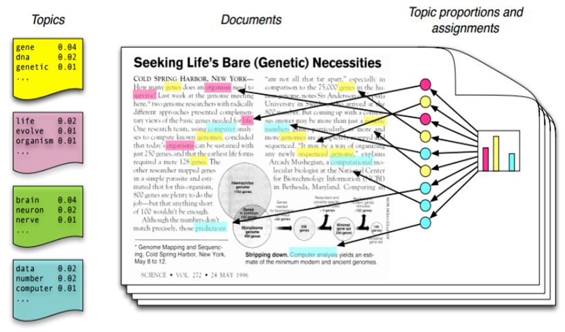
corpora is pre-determined. This process is illustrated with an example in Figure 2.
As can be seen, in this case there are four topics, which are made up of a distribution
of words. Each document is assumed to have a topic distribution as visualized in
the histogram on the right. Based on that, each word is assigned a topic, as seen
by the arrows pointing to the highlighted words.
Figure 2: Intuition behind LDA model from Blei (2012)
Formally, this is done through the generative process:
1. Choose θi ∼ Dir(α)
2. Choose ϕk ∼ Dir(β)
3. For each word in document i of length j
(a) Choose a topic indicator zi,j ∼ Multinomial(θi )
(b) Choose a word wi,j ∼ Multinomial(ϕi,j )
12Where θi is the topic distribution for document i, ϕk is the word distribution for
topic k, wi,j is the j-th word in document i and zi,j is the topic for wi,j .
LDA is an unsupervised model, meaning that it does not require any prior in-
formation (e.g.: tagged data) to infer topics, this causes two main issues. First, it
has been shown that resulting topics in LDA are not always easily interpretable for
humans (Chang et al., 2009). This is especially important in qualitative research,
as it requires interpretable topics. Second, there is no control over what the result-
ing topics are. Therefore, in the case of this study, there would be no assurances
that the stereotypes explored in the literature would appear in the results. For this
reason, seeded topic models are used instead.
Seeded topic models are a semi-supervised version of LDA, which can have cer-
tain topics be defined ahead of time (Andrzejewski & Zhu, 2009; Jagarlamudi,
Daumé III, & Udupa, 2012). More specifically, seed words can be defined for certain
topics to pre-define what the topic should cover. When a topic is given a seed word,
that word is assumed to belong only to that topic (e.g.: the model assumes there is
zero probability of it belonging to another topic). However, a seed word can be used
in more than one topic, in which case it will have equal probability of belonging
to each topic. In terms of the generative process of seeded topic models, only the
second step is different from that of LDA described above. This happens because in
seeded topic models, the word distribution over topics is restricted. That is, certain
words are predetermined to belong to certain topics, and thus, when generating the
word distribution over the topics that must be take into account. Formally, the
second step of the generative process is adjusted to accommodate a restricted ϕ,
which contains the predetermined seed words for selected topics. In this thesis, an
implementation of the model in Java is used (Magnusson & Jonsson, 2021).
The topics to be defined ahead of time and their seed words were chosen based on
previous literature about stereotypes used by the media when reporting on women’s
sports. Based on qualitative studies, five topics were identified: sexualization, fam-
ily, emotions, on-pitch coverage and off-pitch coverage (the seed words used for each
of them can be found on Appendix B).
An important step in this method is deciding on the number of topics to generate.
To do so, it is necessary to evaluate models, so that it is possible to compare how
changing the number of topics affects the results of the model. The most commonly
used measure to asses topic models, which is that suggested by Blei et al. (2003) in
the original LDA paper, is the log-likelihood. For this study, seeded topic models
with 100, 200 and 300 topics were run, and the log-likelihood computed every 100
iterations of the model. Each model had a similar average log-likelihood, of around
−4.89 (need to double check specific values). As it was not possible to determine
13a clear difference between the performance of the models, the decision was made
to use the results of the model with 100 topics. A robustness check was performed
using the models with 200 and 300 topics to ensure that the substantial findings do
not change depending on the number of topics used in the model. The outcome of
the robustness check, which can be found in Appendix C, showed that for all three
models conclusions from the analysis hold.
Once the topics are generated, the topic distribution can be deduced for women’s
and men’s articles. These distributions must be evaluated in order to understand
whether or not they differ, as hypothesis 2 suggests. To do that, two different
methods are used, the Jensen-Shannon divergence, which measures how different
topic distributions are; and the Kolmogorov–Smirnov test, which checks whether
this difference is significant.
3.2.1 Jensen–Shannon Divergence
The Jensen-Shannon Divergence (JSD) measures the similarity between two proba-
bility distributions (Lin, 1991), and has been used before to measure topic models
(Aletras & Stevenson, 2014; Blair, Bi, & Mulvenna, 2020). The JSD is based on
the Kullback–Leibler divergence (KLD), which measures how a given probability
distribution differs from a reference distribution (Kullback & Leibler, 1951). The
KLD is calculated using the following equation:
X P (x)
DKL (P ||Q) = P (x) log2 (1)
x∈X
Q(x)
In Equation 1, P(x) and Q(x) are discrete probability distributions. One issue
with the KLD is that it is asymmetric, meaning DKL (P || Q) 6= DKL (Q || P ). When
comparing the distribution of the topic models this is not ideal, since a single simi-
larity scored is desired. For this reason, the JSD is used instead, as it is a symmetric
divergence score based on the KLD. It is calculated using the equation:
1 1
DJS (P ||Q) = DKL (P ||M ) + DKL (Q||M ) (2)
2 2
In Equation 2, M = 21 (P + Q), or the average between the two distributions.
JSD values range from 0 to 1, where a score of 0 demonstrates two distributions are
identical and a score of 1 that they are maximally different.
Before applying the equation, an additional step is needed to prepare the data.
The resulting distribution from the seeded topic model is a continuous distribution.
14However, to calculate the JSD between articles about women and men, distributions
must be discrete. Therefore, the distribution is discretized through binning. More
specifically, the data is made discrete by calculating the probability that a value falls
within an interval, the intervals are defined by the bins. For example, in the seeded
topic model result a given topic can take any probability of occurring in a document,
making it continuous. By binning, the probabilities are divided into intervals and
grouped together (e.g.: from 0 to 0.1 probability; from 0.1 to 0.2 probability, etc).
Based on that, the probability of a topic occurring in a document is now part of
one of the bins that were created, and the data becomes discrete. It is important to
note that the number and size of the bins can impact the resulting JSD, as smaller
intervals will generate groups with higher probabilities and vice-versa. Thus, a
robustness check must be done to investigate how JSD changes as the size of bins
increases or decreases.
3.2.2 Two Sample Kolmogorov–Smirnov Test
The Two Sample Kolmogorov-Smirnov test (KS-2 test) was created by Smirnov
(1939). It allows for the comparison of two empirical distributions and tests whether
or not they are sampled from the same distribution. The KS-2 test is non-parametric,
meaning there is it does not assume the sample is from a given distribution and does
not require information about any parameters. This is very important in this case,
since there is no knowledge of the true distribution of the topics over the documents.
The KS-2 statistic can be calculated using the following formula:
Dm,n = max |F (x) − G(x)| (3)
x
In Equation 3, m is the size of the first sample, n is the size of the second
sample and F(x) and G(x) are the cumulative distribution functions of the first and
second sample respectively. An illustration of how the KS-2 statistic is calculated
can be seen on Figure 3. The red line represents F(x) and the blue line G(x), two
cumulative distribution functions. The black arrow represents the biggest difference
between the two cumulative distributions, which is in fact the KS-2 statistic.
The null hypothesis, H0 , is that the samples come from the populations that
have the same distribution. The hypothesis is rejected if:
r
m+n
Dm,n > c(α) (4)
m·n
In Equation 4, α is the significance level. Based on the critical value table for
the KS-2 test (Smirnov, 1939), when α is 0.05, the critical value, c(α) is 1.358.
15Figure 3: How to Calculate the Two Sample Kolmogorov–Smirnov Test Statistic
Therefore, the equation above becomes:
r
m+n
Dm,n > 1.358 (5)
m·n
q
Based on Equation 5, if Dm,n is larger than 1.358 m+nm·n
, the null hypothesis is
rejected, meaning that the topic distributions of men’s and women’s articles are not
sampled from the same population.
3.3 POS Tagging
Part-of-speech (POS) tagging is the process through which each word in a corpora
is given a syntactic tag. In other words, by POS tagging a given corpus each
token is labelled with its syntactic property. For example, the word ‘kicked’ would
be tagged as a verb, and the word ‘sunlight’ would be tagged as a noun. This
method can be used for the investigation of hypothesis 2a, 2b, 2c and 4. By POS
tagging the documents in the corpora, it is possible to inspect how often noun,
16pronouns, adverbs, adjectives and verbs are used and check whether hypothesis 1a-c
are supported by the data.
POS tagging is an exercise that can be performed by hand, however there are
also automated implementations of POS taggers which can tag data faster than
humans and as a result be applied to larger corpora. Although automated methods
are faster, it is important to note that, like any other model, they are not always
correct. Thus, when using automated POS taggers, it is important to investigate
their performance. This can be done using annotated corpora, that is, documents
that have been tagged by a human who is knowledgeable in the subject. Said
corpora is tagged by an automated tagger and then the results can be compared to
the annotated documents.
In the case of this study, it would be almost impossible to tag all 127, 728 doc-
uments due to the time required for it. Therefore, the Python package SpaCy
(Honnibal, Montani, Van Landeghem, & Boyd, 2020) is used to POS tag the dataset.
SpaCy’s POS tagger is trained on thousands of annotated documents and uses a
combination of statistical models to predict the syntactic label of a given word.
In order to test the performance of the SpaCy tagger, the Brown corpus is used
(Francis & Kučera, 1979). This corpora was curated and tagged by Francis and
Kučera (1979), who selected 500 documents which were divided between 15 differ-
ent categories. For this test, only one category was used, ‘NEWS’. This is because
the current study investigates news articles and thus, the POS tagger must perform
well in labelling this type of text. If using the entire Brown corpus, documents from
categories such as ‘religion’ or ‘US government’ might affect the performance of the
tagger. The ‘news’ category contains 44 documents, totalling over 100, 000 words,
90.4% of which were correctly labelled by the SpaCy tagger.
3.3.1 Mann–Whitney U test
The Mann-Whitney U (MWU) test is a non-paramatric test that compares two
distributions and determines whether both are drawn from the same population
(Mann & Whitney, 1947). The MWU test is similar to the Student’s t-test, but
does not assume that the distributions are sampled from a normal distribution. The
MW U test is applied using the following method:
1. Put observations from each distribution in one set and order them from small-
est to largest value
2. Assign each observation a rank, based on their position in the ordered set, such
that the smallest value has rank 1, and the highest value has rank n1 + n2
17(a) If two or more values in the ordered set are the same, assign a rank equal
to the midpoint of unadjusted rankings, such that they are all given the
same rank.
i. For instance the ordered set (0, 3, 4, 4, 6) will be assigned ranks (1,
2, 3.5, 3.5, 5) instead of (1, 2, 3, 4, 5).
3. Calculate U-statistic rankings
The U-statistic is calculated using the formulae:
U = min(U1 , U2 ) (6)
Where:
n1 (n1 − 1)
U1 = R1 − (7)
2
n2 (n2 − 1)
U2 = R2 − (8)
2
In Equations 7 and 8, n1 and n2 are the number of observations in samples 1 and 2
respectively; R1 and R2 are the sum of ranks in each sample. Since hypothesis 2a, 2b
and 2c compare whether ratios for one category are bigger or smaller than the other,
a one-sided test is used. For hypothesis 2a, this means that the the null hypothesis,
H0 , is that articles about men’s football will have significantly smaller ratio. As
for hypothesis 2b and 2c, the null hypothesis is that articles about men’s football
will have a significantly larger ratio than women’s articles. The null hypothesis is
rejected if:
U > c(α, n1 , n2 ) (9)
In Equation 9, c(α, n1 , n2 ) is the critical value calculated based on the significance
level α, and the sample sizes n1 and n2 . For the purposes of this study, the critical
value is calculated using Python package SciPy (Jones et al., 2001).
3.3.2 Top Word Analysis
Regardless of how often the media makes use of certain types of words, such as
adjectives and verbs, when reporting on men’s and women’s football, there is a
possibility that the word choice is different. For example, even if the media uses
18adjectives equally often when covering male and female football players, there is
a possibility that the exact adjectives used differ between them. Therefore, it is
important to investigate which words are commonly used used in each word type
category, and whether they differ between reporting on men and women. This is
will give an understanding of the qualitative differences in the reporting for each
gender.
To do so, the 500 most commonly used words for each tag will be gathered
for both men and women. That is, for each word type category (e.g.: adjectives,
adverbs, nouns, verbs) the 500 words that appear most frequently in the men’s
articles are collected, and the same is done with the women’s articles. Then, the sets
are compared with each other, to obtain the most common words in each category
that are different for men’s and women’s articles. More specifically, the 25 most
common words that were unique to a category and tag were selected (e.g.: top 25
verbs that appear in the top 500 verbs of women’s articles but not men’s).
3.4 Bonferroni Correction
When performing hypothesis testing, it is important to consider the number of tests
that are done to a sample. When testing hypothesis 3 and 4, which relate to how
the media reporting changes over time, many different tests will be conducted. In
the case of the syntactical investigation, for example, 19 tests are run, that is, one
per year in the dataset, for each of the three comparisons made, totalling 57 tests.
Therefore, the probability that at least one of the tests is positive will be almost 1.
P (≥ 1 signif icant result) = 1 − P (no signif icant results)
P (≥ 1 signif icant result) = 1 − (1 − α)n. of tests
P (≥ 1 signif icant result) = 1 − (1 − 0.05)57
P (≥ 1 signif icant result) = 0.946
This means that even if all tests are insignificant, there is a 94% chance of observ-
ing one spurious significant result. In order to rectify that, the Bonferroni correction
is applied. This method was introduced by Dunn (1961), and takes into account
the number of tests that are performed in the calculation of the significance level.
More specifically, the Bonferroni correction adjusts the p-values to the following
19significance level:
αold
αnew = (10)
n
In Equation 10, αnew is the significance level used to calculate the p-value af-
ter the correction; αold is the desired significance level for the test, regardless of
correction; and n is the total number of hypothesis tests to be performed.
In the case of the syntactical differences analysis, for example, there are 57 tests
to be performed, at a 0.05 confidence level. Therefore, using Equation 10, the αnew
equates to:
0.05
αnew = (11)
57
The Bonferroni correction will be used in two instances of this paper. First, when
the comparing the topic distributions over time, using the KS2 test. Second, when
analysing how the syntactical differences evolve over time, as mentioned above.
4 Results
4.1 Semantic Gender Differences
In order to get a general overview of the results from the seeded topic model, the
top five topics for men’s and women’s articles are shown on Tables 1 and 2. The
specific words that make up each topic can be found on Appendix D. Firstly, it
can be observed that no topic appears in the top five of both men’s and women’s
football articles. Moreover, it can be seen that three of the main topics about
men’s football regard, to some extent, on-pitch action. ‘Match results’ and ‘on-
pitch’ both cover actions of the game, whereas ‘injuries’ indirectly does the same.
This is because an interest in player’s injuries demonstrates an interest in their
availability to participate in match. The other two topics cover information about
transfer of players between clubs and their contracts. This suggests that there is an
interest in male footballers individually, not just in terms of their performance in
a given club. On the other hand, a large focus exists on female footballers’ private
life, more specifically in their relationships with their families. Other main topics
about women’s football are very general, as is the case of ‘press’ which contains
20Table 1: Most Common Topics For Men’s Football Articles
Ranking Topic Top Words
1 Match Results win 1-0 minutes 2-0 2-1 lead goals 1-1 draw side victory
3-0 minute 0-0 3-1 late put 2-2 defeat beat
2 Transfers club contract deal offer future week move talks agreed
(Contracts) leave yesterday stay confirmed terms understood inter-
est signed agreement agent expected
3 Transfers transfer move deal loan summer sign window signing
(Rumours/Moves) striker midfielder fee january bid player offer interest
free interested defender leave
4 On-pitch goal corner scored penalty chance header performance
scoring free-kick chances updated save ability scores
passing defending passes saved created subs
5 Injuries injury foot injured knee feet form season injuries suffered
leading suspended ankle hamstring scorer subs broke
medical broken doubtful discipline
Table 2: Most Common Topics For Women’s Football Articles
Ranking Topic Top Words
1 Women’s england team game women world cup womens players
Football related womens football usa teams time white australia
girls mens female play tournament top
2 Family big family football day letters son sign relationship email
father quote send wife website boss brother children free
partner
3 Press footballers film story footballer sun celebrity paper daily
press love newspaper star man page tabloid mirror
woman newspapers column pr
4 Football clubs football fa association chief rules government ex-
Entities ecutive professional sport uefa scudamore review issues
national grassroots organisation board health issue
5 Hillsborough police court case death evidence investigation statement
died association found disaster ban appeal report legal
told hillsborough alleged mr
21words such as ‘newspaper’, ‘film’ and ‘star’; and ‘football entities’, a topic with the
words ‘uefa’, ‘fa’ and ‘association’. Finally, the last topic covers the Hillsborough
disaster, an accident that took place in 1989 during a football match at Hillsborough
stadium. This topic is the 7th most common topic in men’s football, and the only
topic to repeat between the two categories in the top 20 of each of them. Therefore,
although this event does not relate to women’s football, the topic appears to be very
important in the corpora, and likely due to the lack of women’s football specific
topics it appears in the top five. Overall, it is seen that the main topics for each
category are very different, providing some support to hypothesis 1.
The Jensen–Shannon divergence values for each topic are shown in Figure 4.
As it can be seen, variations on the size of bins used to transform the data have
little impact on the results. Moreover, it is clear that the family topic displays
the biggest difference in distribution between men and women. Two other topics,
off-pitch and on-pitch, also have small differences in their distribution on women’s
and men’s articles. However, there are also topics, namely sexuality and emotions,
that have a JSD close to zero, suggesting the topic distributions between articles on
women and men are almost identical for these topics. Figure 4 suggests that there
are differences in the topics covered when reporting on men’s football as compared
to women’s football. This provides support for hypothesis 2. However, from the
Figure 4: Jensen–Shannon Divergence For Each Topic For Different Sized Bins
22Table 3: Results for the Two Sample Kolmogorov–Smirnov Test
Topic KS Statistic Critical Value Significantly Different
Sexualization 0.098 0.015 True
Family 0.236 0.015 True
Emotions 0.134 0.015 True
On-pitch 0.122 0.015 True
Off-pitch 0.148 0.015 True
JSD alone it is not possible to understand whether these differences are significant.
To do that, the Kolmogorov–Smirnov Test is needed.
Table 3 displays results for the Two Sample Kolmogorov–Smirnov Test per-
formed on the distributions. As it can be seen, according to the KS-2 test, all
differences observed between the topic distribution of men’s and women’s articles
are significant. This demonstrates that the media reporting is significantly different
between men’s and women’s football when it comes to the five topics explored in
this investigation.
Put together, the measures shows that there are differences between the topic
distributions of articles about men’s and women’s football. This supports hypothesis
2 and indicates that the media does make use of certain stereotypes when reporting
on women’s football. However, these differences are small, especially for certain
topics, such as sexualization and emotions.
These differences might be small because there are changes over time, which do
not appear when studying the data in its entirety. Therefore, the above mentioned
methods are then applied to each year of the dataset to understand how the topic
distributions between men’s and women’s football articles evolves over time. Results
are presented in Figures 5 and 6.
Figure 5 displays how the average JDS per topic changes over the years. It can
be seen that, in general, the differences between women’s and men’s football articles
decreases over time. The turning point appears to be 2013, after which point the
differences start decreasing. As a whole, Figure 5 shows evidence that supports
hypothesis 3, indicating that the distribution of topics between men’s and women’s
football articles decreases over time.
As for the significance of these differences, Figure 6 provides information about
the p-values of the KS-2 tests for each topic for each year in the dataset, adjusted
using Bonferroni correction. Results demonstrate that despite the decrease in differ-
ences between the topic distributions, they remain significant for the topics family
23You can also read