Mandated and voluntary social distancing during the COVID-19 epidemic - Sumedha Gupta, Indiana University Kosali Simon, Indiana University Coady ...
←
→
Page content transcription
If your browser does not render page correctly, please read the page content below
BPEA Conference Drafts, June 25, 2020

Mandated and voluntary social distancing during
the COVID-19 epidemic
Sumedha Gupta, Indiana University
Kosali Simon, Indiana University
Coady Wing, Indiana University
Conflict of Interest Disclosure: The authors did not receive financial support from any firm or person
for this paper or from any firm or person with a financial or political interest in this paper. They are
currently not officers, directors, or board members of any organization with an interest in this paper.
No outside party had the right to review this paper before circulation. The views expressed in this paper
are those of the authors, and do not necessarily reflect those of Indiana University.
MANDATED AND VOLUNTARY SOCIAL DISTANCING DURING THE COVID-19
                                        EPIDEMIC

                Sumedha Gupta            Kosali Simon          Coady Wing
                                       Together with

    Ana Bento, Xuan Jiang, Byungkyu Lee, Felipe Lozano Rojas, Laura Montenovo,

            Thuy Nguyen, Shyam Raman , Ian Schmutte and Bruce Weinberg

                                         Abstract
       During the first half of 2020, the COVID-19 epidemic upended social and economic
  life in the United States. In an e↵ort to reduce the risk of transmission and infection,
  people reduced their mobility and interpersonal contact. State and local governments
  implemented a variety of recommendations, mandates, and business regulations to induce
  higher levels of social distancing. The epidemic and the social distancing response to
  the epidemic have led to very high unemployment. E↵orts to reopen the economy, lift
  social distancing regulations, and return to normal life are underway across the country.
       This paper makes four contributions to the study of COVID19 policy and mobility
  patterns during the epidemic. First, we sketch a simple economic model that highlights
  some incentives and constraints individuals face during the epidemic. Second, we
  provide a typology of the major state and local government social distancing policies
  during the shutdown and reopening phases. Third, we review new data sources useful
  for measuring mobility and contact using cellular device signals. Fourth, we present
  results from event study regressions that can help disentangle private vs. policy-induced
  changes in mobility.
       During the shutdown phase, we find that large declines in mobility occurred before
  states implemented or announced stay-at-home (SAH) mandates, and also in states that
  never adopted SAH mandates. This suggests that a substantial share of the observed
  decline in mobility was a private response to new information about the risk of infection.
  Event studies suggest that first case announcements, emergency declarations, and school
  closures reduced mobility by 1-14% after 5 days and 9-52% after 20 days. Most measures
  of mobility increase by 1% to 4% within five days after a state reopening policy.
       We used our regression results to decompose the trends more formally. For example,
  we find that during the shut down phase, the PlaceIQ mixing index declined by 142
  points. About 65% of that decline is attributable to state emergency declarations;
  secular trends account for the remaining 35%. Likewise, emergency declarations explain
  about 51% of the decline in the SafeGraph measure of hours spent at home during the
  shutdown. In the reopening phase, the mixing index rose by 68 points, and the fraction
  leaving home increased by 10 percentage points. State reopening policies explain almost
  none of the increase in mixing and 31% of the increase in the fraction at home.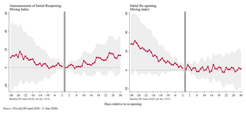
1     Introduction
During the first half of 2020, social distancing has emerged as the primary strategy for
reducing the spread of SARS-COV-2, which is the virus that causes COVID-19. The level of
physical mobility and interpersonal contact declined very steeply in the early months of the
epidemic. More recently, mobility has started to rise again as people resume some aspects of
regular life. The current level of social distancing is partly generated by the private decisions
people make in response to the health threat posed by the epidemic. Governments have also
adopted a variety of mandates and regulations that are intended to reduce mobility even
further. Of course, the production of more social distance is not a typical goal of state and
local governments. There is very little guidance from the academic literature on which policy
levers can produce the most social distance at the lowest economic cost. Existing economic
and public health data systems do not provide much information on patterns of physical
mobility and contact, which makes it hard to optimize social distancing policies in an iterative
fashion. Successful e↵orts to identify principles that can guide the development of social
distancing policy and perhaps develop more targeted social distancing policies could have
substantial value. In a series of research papers, we have measured levels of social distancing
using high frequency data, and assessed the role of state and local public policies in shaping
levels of social distancing. Our over arching goal is to develop knowledge on the underlying
factors that make some distancing policies more e↵ective than others (Gupta et al., 2020;
Nguyen et al., 2020; Montenovo et al., 2020; Rojas et al., 2020; Bento et al., 2020; Gupta
et al., 2020).
    In this paper, we provide an overview of social distancing policies, explain a collection
of new data sources that can be used to track levels of mobility, and present a core set of
empirical results from the shutdown and reopening phases of the epidemic. The paper is
organized in 8 sections. Section 2, gives a short discussion of the emerging literature on social
distancing. In section 3, we sketch a microeconomic model of household production and
choice that incorporates physical contact and infection risk into the agent’s decision process.
The model is very simple and does not reflect key sources of complexity in the real world.
However, it helps clarify the incentives and constraints that a↵ect decisions to engage in
physical contact with others, and it suggests broad principles that might be used to guide
the design of social distancing policies. Section 4 reviews the long list of public policies that
state and local governments have actually adopted during the epidemic, and explains how we
organized and grouped these policies to facilitate empirical analysis. Section 5 provides an
overview of the cell signal based data sources that we are using to measure mobility patterns

                                               1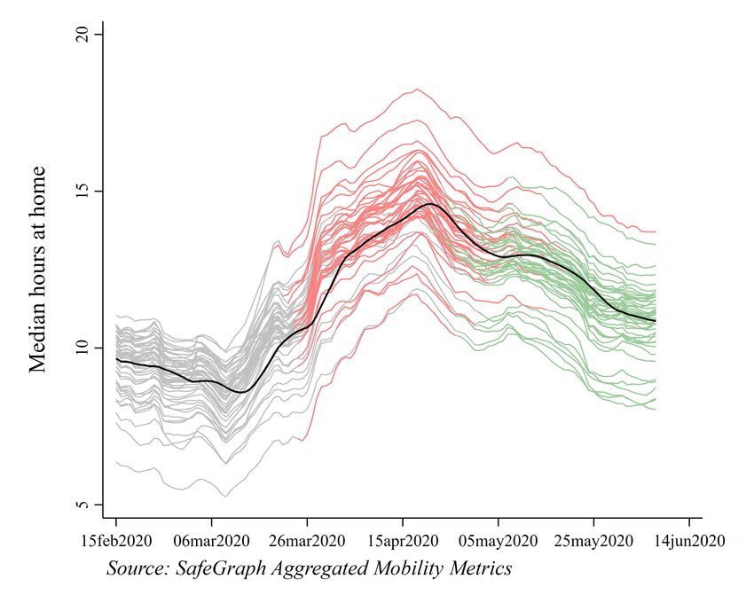
across states and over time. One of contributions is pointing out the importance of looking
at multiple measures of mobility, by showing that take-away messages otherwise vary if one
were to use data only from one source. Section 6 lays out the event study framework we
use in much of our empirical work. We present results in section 7 and o↵er conclusions in
section 8.

2     Related Research
The literature on the design and e↵ectiveness of social distancing policies for managing a
large scale outbreak is growing fast (e,g, Ellison (2020); Papageorge et al. (2020); Dave et al.
(2020); Aum et al. (2020); Simonov et al. (2020); Coibion et al. (2020)), but there is not much
of a literature that existed prior to COVID-19. There is some empirical support for the idea
that social distancing policies can reduce the severity of the epidemic from studies of prior
epidemics in the U.S. and other countries, and from studies of the COVID-19 epidemic in
China (Correia et al., 2020; Fang et al., 2020; Bootsma and Ferguson, 2007; Hatchett et al.,
2007). Of course, the current epidemic is much larger than others in recent history, and
behavioral responses to an epidemic in the contemporary U.S. may di↵er from epidemics in
earlier historical periods or in other countries.
    There are few data systems available to measure the quantity of close physical interaction
at a level of frequency and detail that would be useful in the context of an ongoing epidemic
(Prem et al., 2020). Traditionally, epidemiologists use contact surveys to study interactions
between sub-populations (Kremer, 1996a; Mossong et al., 2008; Rohani et al., 2010; Bento
and Rohani, 2016; Prem et al., 2020). These surveys are sometimes used to parameterize
epidemiological models (Mossong et al., 2008; Rohani et al., 2010; Bento and Rohani, 2016;
Prem et al., 2020). But surveys are expensive and cannot be easily done in a timely manner to
guide ”nowcasting”. Moreover, point-in-time contact surveys are not a useful way of evaluating
the causal e↵ects of mitigation policies adopted during an epidemic, or of monitoring levels of
compliance with social distancing guidelines (Fenichel et al., 2011). Finding proxy measures
of social contact is an important initial objective for policy research related to the epidemic.
    Beyond measurement of the contact and social distancing, the pre-COVID literature
provides little insight into the likely e↵ectiveness of di↵erent policy levers on mobility (Jarvis
et al., 2020; Prem et al., 2020). Over the past several months, researchers have worked
quickly to fill this gap in the literature. A growing number of studies are concerned with
the e↵ects of various social distancing policies on measures of mobility and contact, e.g.
(Andersen, 2020; Painter and Qiu, 2020; Gupta et al., 2020; Nguyen et al., 2020; Montenovo

                                                2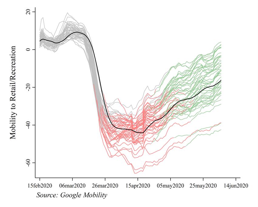
et al., 2020; Rojas et al., 2020; Bento et al., 2020; Gupta et al., 2020); ones that use only
multiple sources of mobility data demonstrate that its important to view these results in
their totality, as specific measures could give varying answers on the importance of policy. A
related literature examines the reduced form e↵ects of the policies on measures on COVID-19
transmission and mortality rates (Kaashoek and Santillana, 2020; Friedson et al., 2020;
Abouk and Heydari, 2020; Courtemanche et al., 2020). Although the emerging literature
is encouraging, identifying the causal e↵ects of public policy changes on first-stage social
distancing outcomes and downstream measures of the severity of the epidemic is not a trivial
exercise and there are many possibly sources of confounding and bias.

3     Theoretical Framework
In epidemiology, the dominant paradigm for analyzing an infectious disease outbreak is the
susceptible-infected-recovered (SIR) model (Kermack and McKendrick, 1927), which examines
dynamics of an epidemic that arise as a population moves through disease relevant states.
These models do not provide much insight into the way that an epidemic might alter the
behavior of people in a population. The economic epidemiology literature nests a micro level
model of individual behavior inside the SIR framework to try to model the role of endogenous
self-protection behaviors might alter the dynamics of an epidemic (Philipson, 1996; Kremer,
1996b; Geo↵ard and Philipson, 1996; Philipson, 2000). A much larger literature in economics
explores individual choices and investments that a↵ect health (Grossman, 1972, 2000). This
literature allows health to a↵ect the utility function directly, and indirectly as an input into
many other activities that people value. A key point is that health is not the only thing
that people value, and it is common for people to make trade-o↵s between health and other
objectives. Indeed, a major sub-field examines the economics of risky health behaviors such
as smoking, drug use, risky sex, poor diet, and dangerous driving (Cawley and Ruhm, 2011;
Viscusi, 1993).
    In this section, we sketch a simple microeconomic model in which a utility maximizing
agent allocates time and resources between activities with di↵erent risks of infection with
SARS-COV-2. The basic model is built on the household production model introduced by
Becker (1965). The starting point is a utility function defined over a set of commodities or
experiences; inputs to the production of these commodities may require physical interaction
with others, which may diminish the production of health. We focus on a utility function
defined over three commodities:

                                               3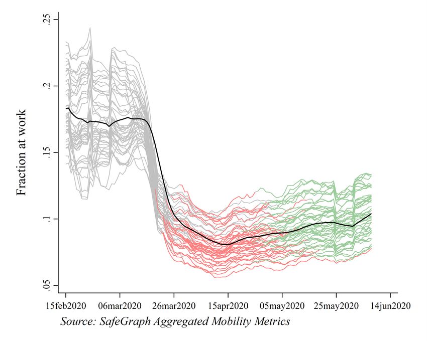
u = u(z, o, h)

    z is a vector of regular commodities, e.g. housing, home-cooked meals, or in-restaurant
dining with friends. o represents market work (occupation), which pays a wage that determines
the value of a person’s time and shapes the person’s budget constraint, but also enters the
utility function directly. h represent a person’s health status.
    Each of the commodities in the utility function must be produced with market goods, time,
and physical interaction with others. To make these relationships concrete, use j 2 z, o, h to
index the three commodities. Let xj be an input vector of market goods that may be used in
the production of commodity j. px is the vector of market prices associated with the market
inputs. ej represents the quantity of a person’s time that is devoted to the production of
commodity j. Finally, dj measures physical interaction with non-household members involved
in the production of commodity j. The person produces z using the production function
z = z(xz , ez , dz ). Similarly, the person produces the market work (occupation) commodity
by combining market goods (e.g. a computer, suitable clothing, a car), time, and physical
interaction with non-household members using a production function o = o(xo , eo , do ).
    The health production function is somewhat di↵erent because it may depend on the
infection risk associated with the physical interactions a person makes in the production of
the other commodities. For simplicity, we assume that all physical interactions generate the
                                                                                           P
same risk, and we ignore spillovers from behaviors of others in the community. Let D = j dj
represent the total amount of physical interaction with non-household members that the
person experiences across all of his home production activities. The health production function
is h = h(xh , eh , ⇢D). In the model, ⇢ is an infectious disease risk parameter normalized so
that ⇢ = 1 for the health risk associated with physical interaction with other people during
                                      @h
”normal” times. We assume that @⇢D       < 0 , which means that health is declining with physical
interaction with other people and with the level of infectious disease risk at that time and
local area.1
    The model sets up a trade-o↵ between health and the production and consumption of
   1
    In our main analysis, we focus on a utility function with a single health commodity. But it is also logical to
view h as a vector of health commodities, each element of which may have a production function that depends
on physical interaction in a di↵erent way. For example, we might say that h = (m, r) is a vector consisting
of mental health (m) and respiratory health (r). Then m = m(xm , em , ⇢m D) and r = r(xr , er , ⇢r D) would
represent mental health and respiratory health production functions. In this case, it might be reasonable
to expect that @⇢@m
                  mD
                       > 0 even though @⇢@r rD
                                                < 0 so that physical interaction improves mental health and
worsens respiratory health.

                                                        4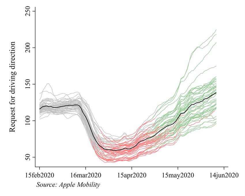
other commodities that raise utility but also require potentially health damaging exposure to
the virus. The COVID-19 epidemic can be viewed as an exogenous change in the prevailing
level of the infectious disease parameter, ⇢. The epidemic does not alter anyone’s utility
function or production technology. But people faced with higher values of ⇢ may nevertheless
choose a new mix of commodities to produce and consume.
    To pay for market goods, at prices px , the person relies on earned and unearned income.
Suppose that M is the person’s non-labor income, w is his/her wage rate, and eo is hours
devoted to occupational work. As above, xj represents the vector of inputs used in the
production of commodity j. The person’s budget constraint is x0z p + x0o p + x0h p = M + weo ,
where eo is the amount of time the person devotes to market work. In addition to the financial
budget constraint, the person has a fixed time endowment so that the sum of his/her time spent
in market work and across the production of various commodities must satisfy T = ez + eo + eh .
The person’s problem is to max u(z, o, h), subject to (i) x0z p + x0o p + x0h p = M + weo , (ii)
T = ez + eo + eh , (iii) z = z(xz , ez , dz ), (iv) o = o(xo , eo , do ), and (v) h = h(xh , eh , ⇢D).
    Writing out first order conditions and solving the system of equations would lead to
a collection of demand functions for each market inputs, time use, and level of physical
interaction with other people. These demand curves are derived from the person’s demand
for commodities (z), occupational work (o), and health (h). Let xz = xz (p, w, F, ⇢) is the
person’s derived demand for market good inputs into the production of z. Likewise, let
ez = ez (p, w, F, ⇢) represent demand for time devoted to the production of z. And let
dz = dz (p, w, F, ⇢) be the person’s demand for physical interaction in order to produce z.
Similar input demand functions are defined for for inputs required to produce the occupational
work commodity (o), and to produce health (h).
    In this framework, the COVID-19 epidemic amounts to an external increase in ⇢, which is
the infection risk generated by physical interaction with other people. Marginal increases
in ⇢ a↵ect utility through the e↵ect of infection risk on health production. However, larger
changes in ⇢ may also generate indirect e↵ects on utility through behavioral changes in the
demand for other commodities, market goods, and time uses. The private responses to the
epidemic are captured by partial derivatives of the various demand functions. For example,
@dj
 @⇢
    is the e↵ect of an increase in infection risk on physical interaction involved in producing
                                             @dj
commodity j. Typically, we expect @⇢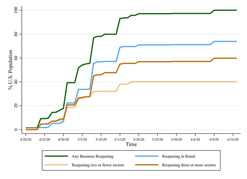
consume in conjunction with physical interaction. The nature of these changes depends on the
commodity production functions. Physical interaction may be a close substitute for market
goods in the production of some commodities. In these cases, an increase in infection risk (⇢)
will increase the demand for substitute market inputs. In other cases, physical interaction and
market goods may be complements in the production function. Then rising infection risk will
tend to reduce demand for the market goods that are complements to physical interaction.
Similar patterns hold for time use. The change in demand for market goods, time use, and
interaction do not flow from a change in preferences. The issue is that people cannot produce
certain commodities as safely as they did in the past. In this sense, the disruption from the
epidemic flows from a negative supply shock.
    Individual reductions in physical interaction may confer benefits on other people. The
positive externalities may justify government policies to promote social distancing. One class
of social distancing policies target physical interactions directly. The government might levy
an a tax on physical interaction, issue advice and mandates that attach stigma to interactions,
or regulate the group size of interactions. These policies will tend to reduce the demand for
physical interaction, but they will also a↵ect the demand for various input goods and services.
    A di↵erent class of policies focuses on market goods that are viewed as strong complements
to physical distancing. For example, the government might levy higher taxes on various kinds
of public transit, admission to parks and beaches, or restaurant meals. Tax instruments
like this have not been widely used during the epidemic. Instead, governments have tended
to mandate that certain types of goods and services may not be sold during the epidemic.
Closing restaurants and bars reduces demand for the input goods directly, but also could
reduce demand for physical distancing which is a complement to visits to these establishments.
    A third class of policies might target the infection risk parameter. For example, govern-
ments might require people to wear masks during physical interactions. A successful mask
policy could be represented as a factor that diminishes the realized e↵ect of the infection risk
parameter. For instance, people wearing masks might produce health using h = h(xh , eh , ↵⇢D),
where 0 < ↵ < 1 is the e↵ect of the mask and the ”e↵ective” infection risk is now ↵⇢ < ⇢. At
current margins, infection risk mitigation policies might increase the demand for physical
interaction and for the goods and services that go along with it. These kinds of policies may
have important economic benefits because they would help resolve the supply shock in the
economy.
    The model we examine here treats infection risk as an aggregate parameter and focuses
on the way that changes in infection risk might a↵ect demand for physical interaction, market
goods, and time use. A richer model would specify a health production function that varied

                                               6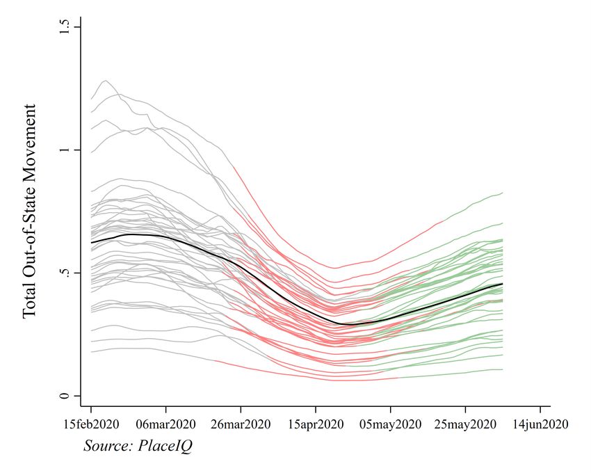
with characteristics of the person, perhaps including factors like age and pre-existing health
conditions that make a person particularly sensitive to COVID-19. In that setting, the
magnitude of private responses to changes in infection risk would vary across people, and
there would be a case for more targeted government interventions that focused not only on
goods and interactions, but also on people with higher health costs of infection.

4       Government Policies During The Epidemic
In this section, we provide an overview and rough typology of the strategies that state and
local governments have used during the shutdown and reopening phase of the epidemic.

4.1     Typology of Policies During Shutdown
We assembled data on state and county level events and social distancing policies using
information from several policy tracking projects, including from the National Governors
Association, Kaiser Family Foundation, national media outlets, Fullman et al. (2020) and
Raifman and Raifman (2020). We began with a large collection of 15-20 separate policies that
are tracked by one or more outlets. However, many of policies, such as state laws banning
utility cancellations for non-payment of bills, are unlikely to directly a↵ect mobility in a
major way. In addition, most tracking services record di↵erent degrees of the same type of
policy, such as gatherings restrictions by the size of the group a↵ected, or closures of di↵erent
types of economic activity. Policy trackers also di↵ered occasionally in whether they followed
only mandates or also reported government recommendations.
    Given the difficulty of estimating e↵ects of a large number of policies at once, one of
our first tasks was to organize and structure data on the core public policy instruments
state governments have been using during the epidemic.2 We reduced the raw number
of policies under consideration by assessing which mandates and information events were
logically connected with individual behaviors related to mobility and social distancing. We
were also guided by the joint timing of policy changes, whether a policy was adopted by a
large number of states, and whether there was concordance about the timing and nature of
the policy across multiple sources.
    Most of our empirical work distinguishes two broad types of state: informational events,
and government mandates. The informational events we consider are the announcement of
    2
    In Gupta et al. (2020) we follow county policy making as well, although there was much less activity on
that front; we focus only on state policies in this current paper.

                                                    7
the state’s first COVID-19 case and death; we collect these dates through the CDC website,
other repositories, and by searching news outlets. Public information events may induce
people to voluntarily engage in individual behaviors that mitigate transmission, including
social distancing, frequent hand washing, mask-wearing. Government mandates consist of a
considerable set of state level policies related to emergency declarations, school and business
closures, and stay-at-home orders. Most of our work revolves around the date at which these
mandates became active. However, we often also consider the data of announcement as a
sensitivity check and to assess the possibility of anticipatory responses. On average, the
announcement and implementation dates were usually about two days apart.
The six state mandates we tracked are listed below, roughly in the order in which they
rolled out across states:
1. Emergency declarations: These include State of Emergency, Public Health Emer-
gency, and Public Health Disaster declarations. All states issued these policies by
March 16th, 2020. The federal government issued an emergency declaration on March
13th, 2020. States may use these declarations in order to pursue other policies such as
school closure, to access federal disaster relief funds, or to allow the executive branch
to make decisions for which they would usually seek legislative approval. By statute,
states are able to exercise additional powers when they issue emergency declarations.
In a typical state, governors are able to declare an emergency, and usually do so for
weather-related cases—although some states, such as Massachusetts in 2014, have
invoked public health emergencies in order to address addiction-related issues in the
state (Ha↵ajee et al., 2014). In some states, city Mayors also may issue emergency
declarations. In our conceptual framework, emergency declarations are typically the
earliest form of state policy that might induce a mobility response; however, we think
that emergency declarations are best viewed as an information instrument that signals
to the population that the public health situation is serious and they act accordingly.
2. School closures: Some school districts closed prior to state-level actions. However,
by April 7, 2020, 48 states had issued statewide school closure rulings(verified through
Fullman et al. (2020) and Education Week (2020)). While school closure policies
would reduce some travel (of children and sta↵), they could reduce adult mobility as
well if parents changed work travel immediately as a result. School closures may also
contribute to a sense of precaution in the community. Although many spring break
plans were cancelled, it is possible we might also capture increased travel due to school
closures.
83. Restaurant restrictions and partial non-essential business (NEB) restric-
tions: These policies were also fairly widespread, with 49 states having such restrictions
by April 7th, according to Fullman et al.. This law would directly restrict movement
due to the inability to dine at locations other than one’s home.
4. Gatherings recommendations or restrictions: These policies range from advising
against gatherings, to allowing gatherings as long as they are not very large, to cancel-
lation of all gatherings of more than a few individuals. There was a lot of action on
this front: 44 states enacted gatherings policies. In principle, these laws would reduce
mobility in a manner similar to restaurant closings. However, gathering restrictions
are hard to enforce and rely on cooperation from residents. Their e↵ects on mobility
patterns is apt to be negligible, and we generally do not focus on these policies in our
empirical work.
5. (all) Non-Essential Business closures (NEB): NEB closures typically occurred
when states had already conducted partial closings and then opted to close all non-
essential businesses. 33 states acted in this area during our study period. NEB closure
could have fairly large e↵ects, as they reduce where purchases happen and also reduce
work travel. Moreover, they provide a binding constraint on individual behavior; even
those not voluntarily complying with social distancing recommendations had fewer
locations to visit.
6. Stay-At-Home (SAH): These policies (also known as “shelter-in-place” laws) are the
strongest and were the last of the closure policies to be implemented. SAH mandates
may reduce mobility in very direct and obvious ways. A few states enacted curfews
specifying the hours when individuals can leave their homes. However, we do not classify
curfew policies as equivalent to SAH mandates. Several states have not issued a SAH
in any part of the state (Vervosh and Healy, 2020); as of April 3rd, these included
Arkansas, Iowa, Nebraska, North Dakota, and South Dakota.
The state policies adopted during the shutdown phase occurred very rapidly. With an eye
towards econometric models, we worked to understand the order and timing of the sequence
of policies and to assess the extent to which it is feasible to meaningfully separate the e↵ects
of di↵erent policies. Figure 1 shows how the share of the U.S. population that was subject to
each social distancing policy evolved over time.3
3
Figure 2.2 in Gupta et al. (2020) shows the timeline of the policy changes that occurred in each state, and
Figure 3.2 shows the timing of the first cases and deaths by state. There we show that the first COVID-19
case in a state is easily set apart in timing from the other policies, as is the first COVID-19 death.
9Emergency Declarations appear early and separate from the other policies. However,
School Closures, Gatherings Restrictions, and Restaurant/Business Closings often coincide
so closely in time that it seems infeasible to separately identify their e↵ects in a regression
analysis. Given the information on the sequence and timing of state policies, we condensed
the seven major policy events in to a set of four major events during the shutdown phase:
State First Cases and Deaths, Emergency Declarations, School Closures, and Stay-at-Home
mandates.
As this section demonstrates, there are some principles we use for selecting which of the
large number of di↵erent state policies currently discussed in the COVID-19 policy literature
we should track in our research on mobility. The key decision factor was ensuring close
connections to our theoretic framework while considering (informally) whether we could
plausibly separate the e↵ects of these policies.
4.2 Typology of Reopening Policies
We collected and coded data on state reopening policies, starting with New York Times
descriptions of reopening plans. We gathered additional information on the reopening
schedules for each state through internet searches.4 We consider two primary reopening dates
- date of announcement of upcoming reopenings and dates of actual reopening. We define the
state’s reopening date as the earliest date at which that state issued a reopening policy of
any type. The dates we arrived at as the first reopening event for each state are identical
to the ones depicted in figures used by the New York Times article. Starting with South
Carolina, by June 15, 36 states had officially reopened in some phased form.
Some states never formally adopted a stay-at-home order, but even these states imple-
mented partial business closures (i.e. restaurant closures) and some non-essential business
restrictions. Of course, measures of mobility and economic activity have fallen in these states
as well because of private social distancing choices. In addition, the lack of an official closure
does not mean that state governments cannot take actions to try to hasten the return to
regular levels of activity. For example, South Dakota did not have a statewide stay-at-home
order, but the governor announced a “back to normal” plan that set May 1 as the reopening
date for many businesses. Our study period to examine the e↵ect of reopenings on mobility
commences on April 15 to ensure that we capture reopenings across all states.
Most reopening policies have been centered around seven areas of economic activity:
outdoor recreation, retail, restaurant, worship, personal care, entertainment, and industry
4
We provide the reopening policies information we have compiled from various sources at
https://github.com/nguyendieuthuy/ReOpeningPlans.
10activities. However, the pace at which states have reopened each of these sectors has varied a
lot. Some states reopened most businesses and industries immediately out of ,5 , while others
have adopted a much more phased approach. Retail, recreation and restaurants have often
reopened first and frequently only at limited capacity.
South Carolina was the first state to reopen on April 20. It was also one of the last states
to adopt a stay-at-home order.6 This April 20 reopening was partial, allowing retail stores to
open at 20% of capacity. By April 30, eight states had reopened to some degree (AL, MS,
TN, MT, OK, AK, GA, and SC). Eight more states reopened on May 1; by May 13, a total
of 36 states had reopened. By June 30th all states have undergone at least the first stage of
reopening. In most of our reopening analyses the study period ends on June 15, which means
that we are able to estimate impacts for at least 30 days post reopening using variation from
all 51 states and DC for Phase 1 and Phase2 reopening polices.
Stay-at-home orders and non-essential business closures are related but distinct. Several
states issued ‘stay-at-home’ mandates after they issued orders closing all non-essential
businesses, or after closing some non-essential businesses (such as gyms) and closing restaurants
for on-site dining (Figure ??). Although for the most part, stay-at-home orders coincided
with orders to close all non-essential businesses, restaurants and other select categories of
business closures started well before stay-at-home orders. Many business closures started in
mid-March, along with school closures (see Figure ??(a)). Timing of reopenings have been
within 24 hours of lifting of stay-at-home orders in only 7 states (Connecticut, Florida, Idaho,
Kansas, Montana, Pennsylvania and Utah, refer Table ?? for details). In the remaining states,
reopening frequently preceded official expiry of stay-at-home orders on average by a month
(32 days).
Figure ?? shows that by June 15 all U.S. states have adopted some form of reopening
policy. However, the pace of reopening has been gradual and varied. Figure ?? shows that by
June 15, nearly 75% of the population lives in states that opened the retail sector, but only
60% are in states that opened 3 or more sectors that we track.7 However, 20 states pursued a
more limited strategy by opening only one or two sectors.8
States that either implemented fewer social distancing measures or implemented those
measures later also tended to reopen earlier, based on time since the first of four major social
5
Alaska, Connecticut, Washington DC, Iowa, Indiana, Louisiana, Maryland, Montana, New Hampshire,
Nevada, South Dakota and Wyoming WY reopened initially by opening 5+ of the 7 sectors.
6
Although it issued an emergency declaration fairly early (March 13), South Carolina did not issue a
stay-at-home order until April 7. (See Gupta et al., 2020).
7
Following the New York Times, we track outdoor recreation, retail, food/drink establishments, personal
care establishments, houses of worship, entertainment venues, and industrial areas.
8
For seven states we could not clearly identify the sectors that would be a↵ected by the reopening decision.
11distancing measures – non-essential business closures, restaurant closures, social gathering
restrictions, and stay-at-home orders or advisories. These results may reflect either a lack
of political desire to engage in distancing or a more limited outbreak (?Adolph et al., 2020;
Allcott et al., 2020) .
5 Mobility Data
The data sets typically used in public health research do not provide high frequency measures
of social interaction. To make progress, our research program has made heavy use of data
from at least four commercial cell signal aggregators who have provided their data for free
to support COVID-19 research. Each company has several di↵erent measures of mobility,
which may capture a di↵erent form of underlying behavior, with di↵erent implications for
the transmission of the virus and economic activity. In addition, each company collects data
potentially from di↵erent sets of app users, and it is possible that some of the cell signal
panels are more mobile than others. Given these complexities, it is important to examine
several measures of mobility both to assess the robustness and generality of a result, and to
provide opportunities to learn from di↵erences in results across measures. In this paper, we
discuss results based on data from Apple’s Mobility Trends Reports, Google’s Community
Mobility Reports, PlaceIQ, and Safegraph.
Apple Mobility Trends. Apple’s Mobility Trends Reports (Apple, 2020) are published
daily and reflect requests for driving directions in Apple Maps. The measure we use tracks
the volume of driving directions requests per U.S. state compared to a baseline volume on
January 13, 2020; no county-level equivalent is available.
Google Community Mobility Reports. We extract state-level measures of mobility from
Google’s Community Mobility Reports (Google, 2020), which also contains county level data.
We use the data that reflect the percent change in visits to places within a geographic area,
including: grocery and pharmacy; transit stations (public transport hubs such as subway,
bus, and train stations); retail and recreation (e.g. restaurants, shopping centers, and theme
parks); places of work and residential (places of residence). The baseline for computing these
changes is the median level of activity on the corresponding day of the week from January 3
to February 6, 2020.
PlaceIQ. We use two anonymized, aggregated location exposure indices from PlaceIQ data,
provided in (Couture et al., 2020): (1) a mixing index that for a given day detects the likely
exposure of a smart device to other devices in a county or state on a given day, and (2)
out-of-state and out-of-county travel indices that measure among smart devices that pinged
12in a given geographic location, the percent of these devices that pinged in another geographic
location at least once during the previous 14 days.
Safegraph. We use Safegraph data to measure the median hours spent at home by devices
as well as the number of devices at the census block group level that are detected at typical
work location during the day or to have left the house. We aggregate these to state by-day
levels.
6 Econometric Framework
Let Yst be a measure of mobility in state s on date t. Es is the start date of a closure/reopening
policy in state s. T SEst = t Es is number of days between t and the adoption date. We fit
the following event study regression model:
P 2 P30
Yst = a= 30 ↵a 1(T SEst = a) + b=0 b 1(T SEst = b) + Wst + ✓s + t + ✏st
In the model, ✓s is a state fixed e↵ect, which capture time-invariant di↵erences in outcomes
across states. t is a date fixed e↵ects, which represents a common trend. Wst is a vector of
state ⇥ day measures of temperature and precipitation which helps adjust for seasonality. ✏st
is a residual error term, and ↵a and b trace out deviations from the common trends that
states experience in the days leading up to and following a given policy event. Standard
errors allow for clustering at the state level.
Our main specifications are based on a balanced panel of states. The models are not
weighted and our estimates reflect the average state rather than the average person. The
composition of states contributing to event study coefficients is quite stable for a range of
30 days before and after the event. The calendar time covered by the event studies varies
somewhat across outcomes and is described along with each set of results. To help summarize
results, we assess the presence of a pre-trend based on the statistical significance of the
pre-policy event study coefficients. In our summary results, we say that a measure exhibits a
pre-trend if at least 30% of the coefficients in the pre-period were statistically significant.
We also use the event study models to decompose the overall change in mobility over
time into a share explained by state level policy changes and a share explained by secular
trends that are not associated with state policies. To understand the counterfactual exercise,
13let ŷst be the fitted value for state s on date t from the estimated event study regression.
These fitted values are a model based estimate of what actually happened in the state. Let
⇤
P30 ˆ
yst = yc st b=0 b 1(T SEst = b) is an estimate the counterfactual mobility outcome that
would have prevailed in the absence of the state policy. We compute the daily cross-state
average of the fitted values and counterfactual estimates to form two national time series
of mobility outcomes. A close correspondence between the realized time series and the
counterfactual time series would indicate that changes in mobility are mainly from secular
trends rather than policy.
7 Results
7.1 Trends in Mobility
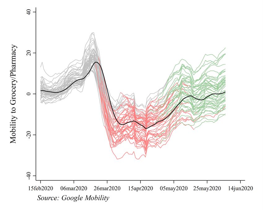
The collection of graphs in figure 2 shows the national and state level time series for a subset
of the mobility measures we follow in Gupta et al. (2020) and Nguyen et al. (2020).The solid
black line indicates the “smoothed” (7-day moving average) national average (not weighted
by state population). Each of the light grey lines represents a state. The state lines turn red
for the time period when a state implemented a stay-at-home (SAH) order, and then they
turn green when a state implements its first reopening stage. This provides a convenient way
to observe when the changes in mobility occurred relative to the policy dates.
The overall pattern of results is very consistent across the di↵erent measures of mobility.
Figure 2a shows the mixing index. Weekend patterns and other seasonal e↵ects are visible,
when all lines move together. There is a substantial drop in mixing around mid-march, when
the index falls 70% between March 1 and April 14. Figure 2 b shows the average “out of
county” travel measure, which fell by 38% between March 1 and April 14. Figure 2g shows
trends hours spent at home, which is a state level average of census block group medians.
Time at home increased 42% increase between March 1 and April 14. The springtime is
typically associated with more mobility and interaction, so any decline during this period is
abnormal.9
The graphs in figure 2 shows that states with no SAH mandates also experienced large
declines in mobility as well as subsequent increases after mid April. Indeed, states with
no SAH policies at all – shown in grey throughout – had declines in movement almost as
9
Data for recent years (2018-2019) from the U.S. Department of Transportation for (seasonally unadjusted)
vehicle miles travelled, shows that the March value is typically 20% higher than February’s value (U.S.
Department of Transportation 2020).
14dramatic as in other states. Furthermore, most states with SAH mandates experienced major
declines in mobility even before the SAH mandates went into e↵ect.
7.2 Mandate E↵ects
Estimates of the event studies evaluating the e↵ect of closure policies and informational
events on each of the mobility measures are presented in Gupta et al. (2020). In Figure 4 we
graphically present the event study coefficients of the e↵ect of state policies and informational
events on the ’mixing index’ available from PlaceIQ Couture et al. (2020). As noted in
Section 5 the mixing index captures the concentration of devices in particular locations
and most closely proxies for social distancing and thus transmission. The results suggest
that the concentration of devices in particular locations does not trend di↵erentially in the
period leading up to any policy or informational event. However, we do not find statistically
significant evidence that the policy or information events have induced substantial changes
in mixing at the state level except for a large e↵ect of emergency declarations. The event
study coefficients imply that emergency declarations reduced the state level mixing index
by about 68% after 30 days, relative to the value of the index on March 1st, which is the
baseline reference period for all percent e↵ects reported for closure events. The coefficients
show a similar pattern for First Deaths, but it is not statistically significant.
Table 1 provides a summary of the results of the event study regressions for each outcome
and policy/information event, including other ones for which figures and tables of coefficients
are reported in Gupta et al. (2020). Table 1 has a row for each state and county outcome
variable, and a column for each policy/information event. The top panel shows the e↵ect size
5 days after the event, expressed as a percentage of the average value of the outcome variable
on March 1, 2020. The bottom panel shows the e↵ect size after 20 days, also expressed as a
percentage of the average outcome on March 1. We bold and indicate with ** the e↵ects
that are statistically significant at the 5% level or better and where parallel trends hold, and
** without bold for significant ones at the 10% level. The cells that are shaded in grey have
possible violations of the di↵erential pre-trends assumption and should be largely overlooked
(we do not indicate statistical significance for them). First death announcements also carry a
large coefficient but it is statistically not significant; school closures and stay at home laws
have statistically insignificant and wrong-signed coefficients.
157.3 Reopening E↵ects
In a manner similar to the event studies for the closure policies, we present results for the
initial reopening dates, starting in figure 4. The two panels display e↵ects first where the
policy date is the announcement of the re-opening, and second for the actual reopening
date. There is a pattern (although not statistically significant) of what appears to be a non-
parallel trend prior to the actual reopening date, but is fairly flat prior to the announcement
date. None of the estimates are statistically significant, even after the policy is e↵ective,
although non-significant coefficients are consistent with an increase in movement after the
announcement date. This helps illustrate our finding that it is important to consider a variety
of mobility measures to assess the impact of the policies. Table 1 shows that although the
mixing index is not statistically precise, there are several other outcomes that are, and do not
violate pre-trends concerns. The e↵ect sizes here are, however, considerably smaller than in
the closure period. One reason for that maybe that in the reopening phase, we do not have
informational events occurring in the same way they did during the closure period. We do
not study the impact of changing rates of COVID-19 cases or deaths, as those were often
directly referred to as conditions for reopening.
The overall message from table 1 for the reopening dates is that estimates are fairly similar
whether we use the announcement date or the actual reopening date, and that e↵ect sizes are
fairly small at both 5 days or 20 days, on the order of 1% to 4%. These are not surprising
results, given the very limited nature of initial reopening phases. The small e↵ects overall
also could mask larger e↵ects in certain situations; event study estimates are summaries of
each state’s experience Wing et al. (2018) and in Nguyen et al. (2020) we show that e↵ects
are larger in states that were the last to close businesses, and also di↵er along a number of
other dimensions.
7.4 The Role of Secular Trends (National sentiment)
One way to interpret our results is to use the event study coefficients to tease apart the
amount of the actual change in mobility that occurred during the closure or reopening time
periods, into shares explained by state actions, relative to secular changes in sentiment due
to other factors. Figure 5 and table 2 show estimates of this decomposition for the mixing
index during the shutdown phase. We used event study regressions to estimate the e↵ects
of emergency declarations on the mixing index outcome. The solid line in figure 5 shows
how the national average mixing index actually changed over time. The dashed line is an
estimate of the counterfactual path of the mixing index, which removes the policy e↵ects from
16the model. The time trends captured by the model imply that in the mixing index would
have increased substantially in the absence of the emergency declarations. 2 shows that the
emergency declaration event study coefficients account for about 65% of the observed decline
in the mixing index that occurred between the first week of March and the second week of
April. The remaining 35% was due to secular trends that occurred separately from state
emergency declarations. Decompositions like this one imply that both policy and private
responses (secular trends) played a key role during the shutdown. However, the specific policy
share vs secular share varies across measures of mobility.
We used this same strategy to examine the state reopening policies. Figure 5 and table 3
show decomposition results for the mixing index and the fraction of people who leave home
during the day. The solid lines in Figure 5 show how the mixing index (panel a) and the
fraction leaving home (panel b) evolved between mid-April and mid-June. Both measures rose
substantially during the reopening phase. The dashed lines show counterfactual estimates of
the path of each index in the absence of the event study state reopening e↵ects. The results
suggest that the reopening policies had almost no influence on the rise of the mixing index.
The growth in that variable is almost completely attributable to a nationwide secular trend
that occurred separately from reopening events. In contrast, the model suggests that state
reopening events did alter the evolution of the fraction leaving home measure of mobility.
Table 3 shows that the fraction leaving home grew from about 60% to 70% between late
April and mid-June. About 31% of that increase is attributable to the reopening policies.
The remaining 69% of the change would have happened even in the absence of state policies,
given the common trends implied by the model. These results again suggest that both private
responses (secular trends) and state level policies have played a role in generating recent
increases in mobility, however the magnitude/share of policy e↵ects varies across measures of
mobility and the policy share is perhaps somewhat smaller during the reopening phase than
during the shutdown phase.
8 Conclusion
We examine human mobility responses to the COVID19 epidemic and to the policies that
arose to encourage social distancing. A simple theoretic framework suggests that individuals
social distance in reaction to information and apprehension regarding the virus, not just in
response to state closure or reopening mandates. We examine closures first, finding that
information-based policies and events (such as ..) had the largest e↵ects, while stay at home
orders do not. This does not imply that these laws would always have such impacts, as
17it is possible people simply react to the earliest of the policies, and stay at home orders
happened fairly late in the time span. Early state policies appeared to convey information
about the epidemic, suggesting that even the policy response mainly operates through a
voluntary channel. Given that most states have now undertaken some form of steps to reduce
the lockdown, we are able to compare mobility during the closure to mobility during the
reopenings. Even though the reopenings are graduate, often with capacity limits for each
sector,we find that mobility increases a few days after the policy change and that other
factors, such as temperature and precipitation also strongly imply increased mobility across
counties. It appears individuals especially increase their visits to a variety of locations, rather
than increase the total time they are outside their home. Finally, we observe that largest
increases in mobility occur in states that were late adopters of closure measures, and thus
had these mandates in place the shortest length, suggesting that closure policies may have
represented more of a binding constraint in those states. Together, these four observations
provide an assessment of the extent to which people in the U.S. are resuming movement and
physical proximity as the COVID-19 pandemic continues. Given the high costs of broad
closures, it behooves researchers to examine possible tagetted approaches.
189 Tables and Figures
Figure 1: U.S. Population covered by State Closure and Re-opening Policies
(a)
(b)
Note: Author’s compilations based on several sources. Data covered January 20, 2020 - June 15, 2020.Figure 2: Trend in mobility changes.
(b) Average out-of-county move-
(a) Mixing index.
ment.
(c) Requests for driving directions (d) Fraction at Work
(e) Retail and recreation (f) Grocery and pharmacy
(g) Median hours at home. (h) Fraction leaving home.
Note: Author’s calculation based on data from Apple Mobility, Google Mobility, SafeGraph Aggregated Mobility Metrics
and PlaceIQ smart device data. Each grey line represents a state, which turn red after the state implements stay-at-home
18
orders and green after phase 1 of reopening. The thick black line represents a “smoothed” 7 day moving average of the
states.Figure 3: E↵ects of Mitigation Policies and Information Events on Mixing Index. Regression
Results (Coefficients and 95% Confidence Intervals)
Note: The dependent variable shows the state’s index for mixing (average amount of mixing within its
census block groups). Standard errors are clustered at the state level. Full event study estimates available
in Gupta et al. (2020).
19Figure 4: E↵ects of Announcement and E↵ective date of initial reopening on Mixing Index.
Regression Results (Coefficients and 95% Confidence Intervals)
Note: Note: The dependent variable shows the state’s index for mixing (average amount of mixing within
its census block groups). Standard errors are clustered at the state level. Full event study estimates
available upon request.
20Table 1: E↵ect Sizes: Percentage magnitude e↵ects of the policy/informational events on
social distancing measures.
I: E↵ects of Mitigation Policies and Informational Events
First Confirmed Emergency School Stay-atHome First Death
Case (FCC) Declarations (ED) Closure (SC) (SAH) (FD)
E↵ects After 5 days
Mixing Index 1% -14%*** 4% -7% -11%
Median Hours at Home -1%* 6%*** 1% 5% 3%*
Fraction Leaving Home 1%** -1%* -1% -5% -2%***
Total Out-of-State Movement -2% -1% -4%** -1% 0%
Total Out-of-County Movement -1% -2%** -4%*** -3% -2%
E↵ects After 20 days
Mixing Index -10% -52%*** 13% -8% -31%
Median Hours at Home -2% 27%*** 3% 11% 9%**
Fraction Leaving Home 2% -13%*** -3% -9% -7%***
Total Out-of-State Movement -9% -3% -13% 1% 5%
Total Out-of-County Movement -2% -8%*** -9%*** -2% -6%*
II: E↵ects of State Initial reopenings
Announcement of
Initial Reopening Initial reopening
E↵ects After 5 Days
Mobility Measures
Request for driving directions -6% -3%
Mobility to retail/recreation 3% 3%
Mobility to Grocery/Pharmacy 8% 9%
Mobility to Transit Stations 0% 9%
Mobility to Workplace 2% 3%**
Fraction at Work -3%* 2%
Fraction left home 1%** 1%**
Mixing Index -2% 5%
Out of state movement -2% 0%
Out of county movement -1% 0%
Absence of Mobility Measures
Stay in Residential Areas -1% -4%**
Median hours at home -1%* -1%***
E↵ects After 20 Days
Mobility Measures
Request for driving directions -15% -15%
Mobility to retail/recreation 8% 4%
Mobility to Grocery/Pharmacy 8% 4%
Mobility to Transit Stations 0% -6%
Mobility to Workplace 4% 1%
Fraction at Work -2% 1%
Fraction left home 4%*** 1%
Mixing Index 20% -4%
Out of state movement -1% -8%
Out of county movement 2% 0%
Absence of Mobility Measures
Stay in Residential Areas -5% -4%
Median hours at home -3%*** -3%***
Note: Each cell is from a separate regression. *** and bold text denotes e↵ect sizes with p-valuesFigure 5: Change in Social Distancing (Mixing Index) Attributed to Emergency Declarations.
Note: Note: Corresponding to Figure 4, Figure 5 shows calendar time trends of the predicted lines with
and without the policy event time terms set to zero, for the Mixing index measure of mobility, and the
Emergency Declarations policy measure.
Table 2: Estimated E↵ects of Emergency Declarations on Mixing Index.
February 26 - March 3 April 8 - April 14 Change
Actual Mixing Index 194.3 51.9 -142.4
Counterfactual Mixing Index (No policy) 194.3 144.9 -49.4
Secular share of change 0.35
Policy share of change 0.65
Note: Author’s calculation based on decomposition of changes in mobility to share attributable to state
emergency declarations and those resulting from secular trends. Related estimates plotted in Figure5.
22Figure 6: Change in Social Distancing (Mixing Index and Fraction Leaving Home) Attributed
to Initial Reopening.
(a) Estimated E↵ects of Initial Reopening on Mixing Index.
(b) Estimated E↵ects of Initial Reopening on Fraction Leaving Home.
Note: Corresponding to Figure5, Figure 6(a) shows calendar time trends of the predicted lines with and without the policy
event time terms set to zero, for the Mixing index measure of mobility, and the Emergency Declarations policy measure.
Figure 6(b) provides specific values discussed in the text.
23Table 3: Estimated E↵ects of Reopening on Social Distancing.
April 17 - April 23 June 10 - June 16 Change
Actual Mixing Index 53.2 121.2 68.0
Counterfactual Mixing Index (No policy) 53.2 121.5 68.3
Secular share of change 1.0
Policy share of change 0.0
Actual Fraction Leaving Home 0.6 0.7 0.1
Counterfactual Fraction Leaving Home (No policy) 0.6 0.7 0.0
Secular share of change 0.69
Policy share of change 0.31
Note: Author’s calculation based on decomposition of changes in mobility to share attributable to state
initial reopening policy and those resulting from secular trends. Related estimates plotted in Figure6.
24You can also read