Monetizing the Economy: National Banks and Local Economic Development
←
→
Page content transcription
If your browser does not render page correctly, please read the page content below
Monetizing the Economy: National Banks and Local
Economic Development *
Chenzi Xu He Yang
July 2021
Abstract
This article examines the role of banks in expanding the traded sector of local economies
in the United States in the 19th century. The National Banking Act of 1864 created
a new class of better-capitalized banks that issued riskless liabilities that circulated
as a more stable transactions medium. The improved liquidity of their liabilities was
especially important for long-distance exchange. In order to identify the causal impact
of this financial change, we use the regulatory feature that national banks faced cap-
ital requirements defined by town population cut-offs. Using the capital requirement
discontinuity as an instrument for national bank entry, we find that the composition of
agricultural production shifted from non-traded crops to traded crops and that employ-
ment in trade-related professions and businesses grew. Counties with access to national
banks also experienced significant manufacturing output growth from sourcing more
inputs, and they innovated more in product markets. These results are consistent with
the change in the financial sector improving locations’ market access.
JEL classification: E42, E51, N11, N21.
* First version: November, 2018. Previously circulated as “National banks and the local economy.” The authors thank
Anat Admati, Philip Ager, Brian Beach, Asaf Bernstein, Michael Bordo, John Campbell, Lauren Cohen, William Diamond,
James Feigenbaum, Andrew Garin, Michela Giorcelli, Claudia Goldin, Walker Hanlon, Christopher M. Meissner, Nathan Nunn,
Siddharth George, Robin Greenwood, Alberto Manconi, Adrien Matray, Santiago Perez, Sarah Quincy, Tzachi Raz, Hugh
Rockoff, Jann Spiess, Jeremy Stein, Adi Sunderam, Alan M. Taylor, as well as participants at Harvard, Yale, UC Davis,
Einaudi Institute, and the AEAs for helpful comments. We are grateful for financial support from The Lab for Economic
Applications and Policy (LEAP) at Harvard as well as Harvard Department of Economics Summer Research Fellowship.
Stanford GSB. Email: chenzixu@stanford.edu.
Amazon. Email: heyang.um@gmail.com.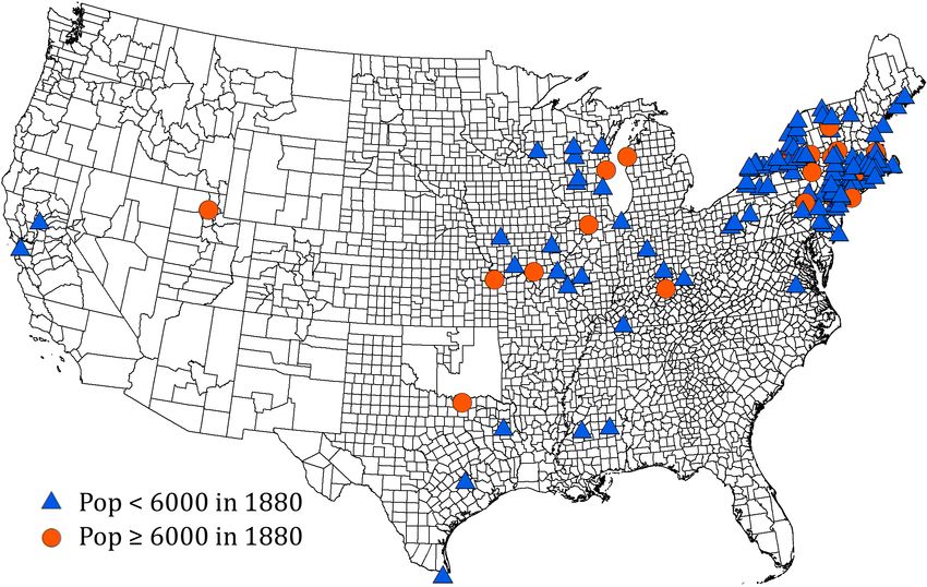
1    Introduction

           Local economic activity rarely exists in autarky and instead usually relies on the ability
    of firms to source inputs for production and sell other inputs and final goods to distant
    markets. This reliance on trade, even in a domestic setting, suggests that local economies
    will be sensitive to changes in intra-national trade costs.1 While there has been much focus
    on the impact of changes in physical trade costs on economic activity, substantial evidence
    indicates that these are likely only a small component of overall trade costs, and that other
    frictions play a much bigger role overall (Anderson and Van Wincoop, 2004).
           In this paper, we focus on the impact of reducing trade costs stemming from changes in
    the financial sector. In particular, we study a key reform to the United States banking system,
    the National Banking Act of 1864, which differentially reduced the financial frictions that
    exacerbated non-physical trade costs for local economies. This setting allows us to provide
    causal identification showing that reducing those frictions generated growth and shifted the
    composition of local activity toward more traded sectors.
           While there is a large literature on the importance of financial intermediaries in eco-
    nomic growth, most studies focus on a direct financing channel—i.e. the extent to which
    individual firms are credit-constrained. However, banks provide more than just credit to
    firms, and our historical setting provides us with an opportunity to examine whether their
    ability to create liquid assets and liabilities can be particularly beneficial for information-
    sensitive long-distance (i.e. trade) transactions (Gorton and Pennacchi, 1990; Stein, 2012).2
    Causally establishing these channels is challenging because financial institutions are not al-
    located randomly and local economic conditions are likely correlated with the characteristics
    of the bank itself. In addition, these indirect roles are often difficult to observe, as they are
    not balance sheet items.
           In our setting, the National Banking Act (NBA) created a new class of federally-
    regulated “national banks” that operated alongside previously existing “state banks.” Two
    characteristics of the setting help us to overcome the challenges to causal identification. First,
    national banks faced capital requirements according to town population cut-offs. Banks
1
  Indeed, during the latter half of the 19th century, the United States benefited from increased market inte-
  gration stemming from the expansion of transportation technologies like railroads that significantly reduced
  physical trade costs and led to substantial growth (Donaldson and Hornbeck, 2016; Hornbeck and Rotemberg,
  2019).
2
  For example, their choices about who gets credit impacts the aggregate (mis)allocation of capital in the
  economy (Bau and Matray, 2020), and they produce information that can alter firm behavior (Frydman and
  Hilt, 2017).

                                                      1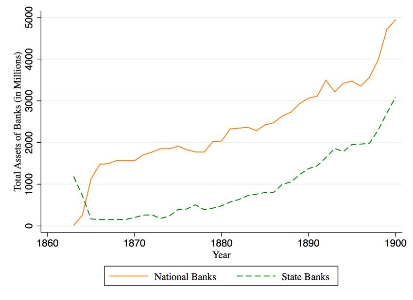
established in towns with fewer than 6,000 people needed to raise $50,000 of capital, but
    banks in towns with more than 6,000 (and fewer than 50,000) people were required to raise
    twice as much. The discontinuous jump means that towns just below the population cut-
    off faced significantly lower entry costs per capita for establishing a national bank. These
    town population requirements were binding since banks were not allowed to branch, and this
    feature of the regulatory environment creates a plausibly exogenous entry cost for new banks
    in towns near the population cut-off.
           Second, the money supply during this period primarily consisted of privately printed
    bank notes that, in conjunction with deposits, were their main balance sheet liability. Prior
    to the NBA, these liabilities were not guaranteed to be redeemable for specie if a bank failed
    nor did they have status as legal tender. As a result, there was significant uncertainty over
    the value of bank notes, and they primarily circulated locally and traded at a discounts across
    town borders (Gorton, 1999). This illiquidity made them unsuitable for trade transactions.
    In contrast, the NBA mandated that all national bank notes were backed 110% in government
    bonds, and that they be redeemable at any other national bank around the country. These
    two features transformed national bank notes into riskless liabilities that were significantly
    more liquid and information-insensitive.
           Gaining access to a national bank therefore altered the financial frictions that a local
    economy faced. First, it directly increased the supply of liquid liabilities (bank notes) cir-
    culating locally. Second, it indirectly increased the town’s “market access” by eliminating
    monetary transactions costs with any other town in the country that also had a national
    bank. Third, while national banks were not allowed to take land as collateral and therefore
    mostly did not lend to the agricultural sector, they did specialize in short-term loans to the
    manufacturing sector, which could overcome direct trade-related financing constraints.3
           We use the different regulatory capital requirements as an exogenous source of variation
    in gaining a national bank by instrumenting for bank entry with town population being below
    the 6,000 threshold, according to the most recently published census. We focus on the towns
    that gained a national bank for the first time in order to capture the impact of joining the
    national banking network.
           Our sample consists of towns that had fewer than 6,000 people in 1870 and no national
    bank as of 1875, and had between 4,000 and 8,000 people in 1880.4 Choosing a small
3
  Trade is more dependent on external finance because of the lags between when goods are produced, shipped,
  received, and paid for. While this constraint has mostly been documented in international trade (e.g. Manova
  (2013); Xu (2019)), it applies in any setting with long communication and transportation lags, such as in
  the US in the 19th century.
4
  The analysis is not sensitive to choosing 1875 as the first year we calculate whether a town has a national

                                                      2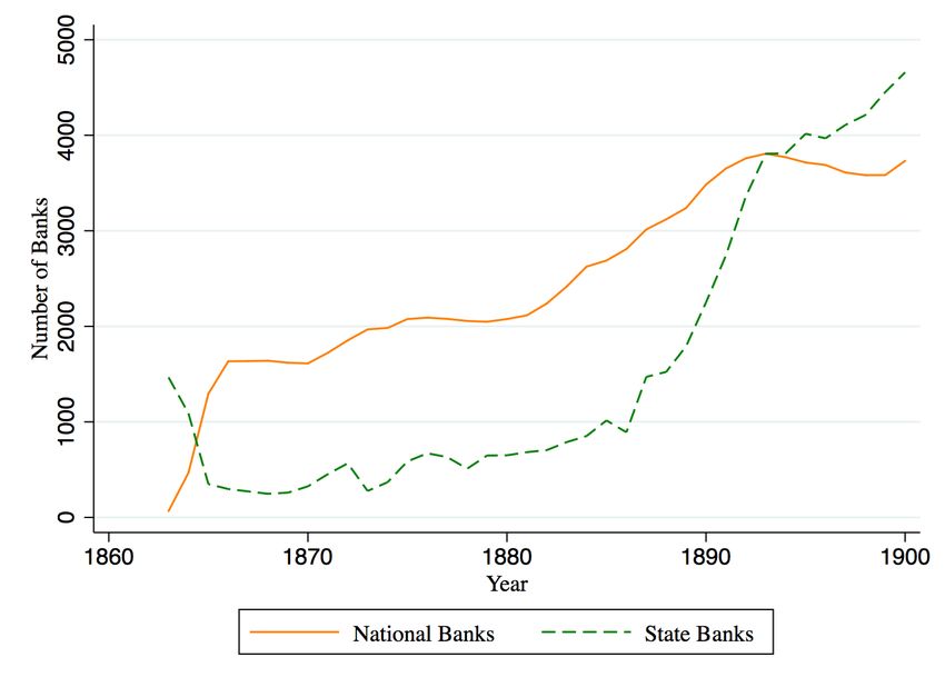
population bandwidth of 4,000–8,000 allows us to limit our sample to towns that are likely
    to be similar in both observable and unobservable characteristics. Among these similar
    towns, some crossed the 6,000 population cutoff in the 1880 census, which doubled the entry
    cost for a national bank. The identifying assumption is that there was not a concurrent shock
    to lower-populated places that would cause them to grow faster after 1880. We control for
    observable differences in their growth trajectory as proxied by population growth, a town’s
    financial development in the pre-period as proxied by the number of state banks in the town,
    as well as the area’s physical trade costs as proxied by the number of railroads in the county.
    The predicted first stage is that towns that did not cross the population threshold should
    be more likely to establish a national bank.
           We show that our instrument strongly predicts the likelihood of a town having a na-
    tional bank in the mid-1880s: having fewer than 6,000 people in 1880 is associated with
    30% higher probability of gaining a national bank as of 1885.5 Controlling for a town’s
    growth trajectory in the pre-period greatly alleviates endogeneity concerns with the rela-
    tionship between population levels in 1880 and future growth in these places. We also show
    that pre-period observable characteristics were not significantly different between the towns
    with a population above 6,000 versus those had below 6,000 population in 1880, both condi-
    tionally and unconditionally. The balance on observables further suggests that selection on
    unobservable characteristics is less of a concern.
           Having established that lower regulatory capital requirements increased bank entry, we
    first show that national bank entry significantly shifted the composition of goods produced
    toward traded goods while not affecting total agricultural production. Output of traded crops
    (those listed on the Chicago Board of Trade), such as wheat and oat, crowded out non-traded
    crops, such as rye and barley. The pure compositional change avoids confounding effects from
    other bank activities that would also affect the levels of production. It is consistent with
    the evidence that the regulatory restriction against lending to the agricultural sector was
    binding (Knox, 1900). We also find that national bank entry did not impact agricultural
    capital that was financed by short-term credit (proxied by fertilizers expenditure) or long-
    term credit (proxied by the value of land and fixtures on farms). Indeed, while direct lending
    was unaffected, the shift toward traded products is a predicted outcome from gaining access
    bank. We show robustness to other years in the appendix.
5
    This finding are consistent with Fulford (2015), Gou (2016) and Carlson et al. (2018) which also use the
    population cut-offs governing national banks’ regulatory capital requirement in the late 19th and early 20th
    centuries. This result follows an older literature by Sylla (1969) and Sylla (1982) that the high capital
    requirements imposed by the National Banking Act hindered financial development.

                                                         3
to a more liquid medium exchange that reduced transactions frictions.
We further demonstrate the positive impact of national banks on trade using direct
measures of local trade activity as proxied by employment in trading sectors. In particular,
we use contemporary business directories with town-level coverage and the full count Cen-
suses of Population to show that there was a relative increase in the number of commission
merchants, buyers, and shippers in places that gained national banks. We also show that
placebo professions that might capture general growth, such as architects and doctors, did
not differentially benefit from gaining a national bank.
Next, we study the impacts of national banks on the manufacturing sector, as manufac-
turing products are also tradable and therefore the sector likely benefited from the increased
trade activity following national bank entry. We use the decennial Census of Manufactures
to show that places that gained a national bank experienced significantly greater growth
in total production between 1880 and 1890. Accessing national banks caused counties to
increase their manufacturing output by 50% relative to 1880 levels. These results are robust
to accounting for financial development and physical trade costs proxied by the number of
state banks before 1880 and the number of railroads in 1880.
The growth in manufacturing output appears to be driven by growth in inputs and
employment whereas manufacturing capital was not significantly affected. These results
suggest that national banks were unlikely to have facilitated growth through extending long-
term loans for capital acquisition.6 Instead, outputs growth was likely driven by short-term
working capital and liquidity provision operating through the assets side of the balance sheet,
as well as transactions costs reduction in inputs and outputs trading operating through the
liabilities side.
These reductions in non-physical trade costs from the financial sector are consistent
with increases in a location’s market access (or “real market potential” (Head and Mayer,
2004)). This measure captures the ease of trading with other markets, and it is a source of
agglomeration forces in the economic geography literature (Redding, 2013). Consistent with
those models, increases in market access that increase firm activity and output also manifest
in increased product market competition. We use the number of patents across counties
as a proxy for manufacturing sector product development (R&D) and find that places that
gained national banks had more innovation by local inventors.
Lastly, we find that the elevated levels of production persisted until the 1900s.7 The
6
This result is consistent with Fulford (2015).
7
The county-level data on manufacturing do not exist for 1910, and the levels are no longer significantly
different by 1920. Given the large amount of changes that likely occurred in WWI, we stop our analysis on
4initial growth in conjunction with the growth in trade and innovation may contribute to
the persistence. In particular, the short-term changes in trade and innovation activity likely
gave places with national banks a comparative advantage in the manufacturing sector over
a longer period.
Our identification strategy follows a number of papers studying bank behavior in the
postbellum United States, and in particular those that use the regulatory capital require-
ments based on population as a source of exogenous variation. For example, Gou (2016)
uses the introduction of a new population cutoff in the early 20th century to study the effect
of capital requirements on bank stability. Similarly to Fulford (2015) and Carlson et al.
(2018), we focus on the 6,000 cutoff in the 1880 census, and as in Carlson et al. (2018) we
also control for town population growth following the previous census as a proxy for a town’s
overall growth trajectory. Unlike Fulford (2015), we use a more geographically disaggregated
unit than the county, and in contrast to Carlson et al. (2018), we focus on towns that gained
a national bank for the first time rather than incumbent entry.8
This paper provides empirical evidence that financial intermediation can meaningfully
reduce trade costs and thereby positively impact real economic activity. In contrast to
Xu (2019) which focuses on a direct financing channel of credit provided to firms, here we
show that an indirect channel of providing secure and stable bank liabilities as a form of
transactions medium also plays a role. While the large literature on the importance of bank
debt liquidity has mostly focused on their fire-sale externalities and their role in raising
financial fragility (Diamond and Dybvig, 1983; Stein, 2012; Admati and Hellwig, 2014), this
paper studies a context in which they are truly safe assets (backed by federal bonds) and
therefore create a Gorton and Pennacchi (1990)-type transactions medium.9 In that sense,
we provide evidence for a sub-national monetary channel in the tradition of Friedman and
Schwartz (1965); Romer and Romer (1989).
Furthermore, this paper adds to the literature of the historical determinants of eco-
nomic growth in the United States. This literature has focused on various factors, such as
the long-term effect at 1900.
8
The concurrent work by Carlson et al. (2018) focuses on the role of bank competition and thereby requires a
different sample of towns. Their analysis primarily focuses on the asset side of the balance sheet and shows
implications for bank lending behavior, leverage, and survival during the 1893 Panic.
9
Quadrini (2017) develops and calibrates a multi-sector model to show how the financial intermediation sector
can impact productivity through the bank liability channel. In his paper, bank liabilities provide insurance
for economic agents who become less constrained in their investments, which is different from our monetary
channel. Kashyap et al. (2002) study the synergy between lending and deposit-taking in liquidity provision,
and Pennacchi (2006) shows that the federal safety net provided by deposit insurance promotes banks’ ability
with liquidity provision. Our paper does not study the implication of stable bank liabilities on lending.
5technological innovations that reduced transportation costs (e.g. Donaldson and Hornbeck
(2016)), information acquisition costs (e.g. Feigenbaum and Rotemberg (2014)), or changes
in demographics (e.g. Sequeira et al. (2018)). This paper is complementary, and contributes
to the better understanding of how the banking sector has impacted economic activities in
the late 19th century (Rousseau and Wachtel, 1998; Rousseau and Sylla, 2005; Landon-Lane
and Rockoff, 2007; Fulford, 2015; Carlson et al., 2018; Weiss, 2018).10 In particular, our
results are consistent with Sylla (1982), which argues that the National Banking Act’s high
regulatory capital requirements held back economic development by failing to expand the
bank note supply sufficiently.
The rest of the paper is organized as follows. Section 2 discusses the historical context
around the time period studied, and provides motivating facts for the assets and liabilities
channels. Section 3 explains the data collection, sample construction, and the empirical
strategy. Section 4 presents the empirical results on the effect of national bank entry on real
economic outcomes, such as production in the agricultural and manufacturing sectors, local
trade activity and innovation output. Section 5 concludes.
2 Historical Context
2.1 The Free Banking Era
Between the expiration of the charter of the Second National Bank in 1836 and the
establishment of the Federal Reserve system in 1913, there was no unified banking system in
the United States.11 The National Banking Act of 1864 marked an intermediate step when
federally-regulated banks operated alongside state-regulated banks. The period before the
National Banking Act was the Free Banking Era. During the Free Banking Era, bank were
chartered by their states (or operated without charters) and were subject to different regu-
lations. State banks were prevented from branching, and interstate banking was forbidden.
Regulatory oversight was generally weak, and bank runs and failures were frequent (Grada
and White, 2003). There was no formal system of interbank lending nor a lender of last re-
sort, and the banking sector experienced regular periods of booms and busts.12 As a result,
10
Both Fulford (2015) and Carlson et al. (2018) attribute the impact of national banks to the credit channel
on the asset side of the balance sheet. While Fulford (2015) studies rural counties that gained national banks
for the first time, Carlson et al. (2018) studies the role of competitive entry on incumbent banks’ lending
behaviors.
11
See Appendix C for more historical background on the First and Second National Bank before the Free
Banking Era.
12
There were two exceptions: the Suffolk Banking System that served New England banks between 1827 and
1858, and a nonprofit collective founded in 1853 (Weber, 2012).
6the antebellum banking system was fragmented, loosely regulated, and local economies were
exposed to the conditions of their local banks.13
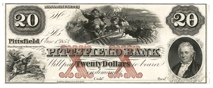
A well-known feature of the Free Banking Era was that banks issued their own bank
notes which were only redeemable at face value in specie at the originating bank’s office.
In 1860 on the eve of the Civil War, there were almost 1,600 state banks, each issuing its
own bank notes. In large cities, the notes from hundreds of banks circulated at any given
time. The fact that there were so many bank notes in different designs means that they
were hard to verify and subject to counterfeit. Publications known as “Bank Note Reporters
and Counterfeit Detectors” were crucial for determining the legitimacy of a currency. Figure
A.1(A) displays an example of a private bank note from Massachusetts with face value $20,
where the name and location of the issuing bank is prominently displayed. Figure A.1(B)
shows the written description for the same bank’s notes in a printed “counterfeit detector,”
where the $20 bill is described in the bottom left corner.
The lack of regulatory oversight from state legislations meant that banks often issued
notes beyond their redemption capabilities, causing uncertainty in the value of their bank
notes.14 Due to the asymmetric information in bank notes value and the physical redemption
costs, the bank notes did not generally trade at par with each other, creating numerous and
constantly changing exchange rates among the currencies (Gorton, 1999; Ales et al., 2008).
The large volatility in state bank notes value over time also indicates significant time-varying
idiosyncratic bank risks. For example, Figure 1 plots average discounts of state bank notes in
several states relative to banks in Philadelphia.15 Despite the relatively low cost of acquiring
information on the state banks in nearby regions, the discounts and premiums were as high
as 10% (Figure 1(A)).
The discounts were more extreme for banks located farther away, as it became more
costly to verify the operational status of those banks, with information asymmetry increasing
with distance (Gorton, 1999). Figure 1(B) plots the average state bank notes discounts for
four states farther away from Philadelphia. The discounts were as high as 80%, which meant
that a bank note with face value of $1 in Mississippi would only be worth $0.2 in Philadelphia.
The final cost of buying goods in Philadelphia with Mississippi bank notes would therefore
13
See Rockoff (1991) for a comprehensive review of the key characteristics of the Free Banking Era.
14
Milton Friedman referred to the phenomenon of banks over-inflating their currency to the point of not being
able to meet redemption as ‘wildcat banking,’ a term that is now frequently applied to the Antebellum
period in American banking. Gorton (1996) shows that discounts on bank debt can also arise from a lack of
credit history.
15
This data is collected in Ales et al. (2008) and the original source is Van Court’s Bank Note Reporter and
Counterfeit Detector published monthly in Philadelphia between February 1839 and December 1858.
7be five times the nominal price. Furthermore, under the unit banking structure, local price
shocks could also easily lead to more bank failures (Bordo, 1998).
The high levels of relative discounts were sometimes due to falling state bond prices
(Rolnick and Weber, 1982) or the anticipation of state bank failures. For example, Illinois
banks committed over 5 million dollars between 1836 and 1842 to building a canal that
would connect the Illinois River and Lake Michigan, hoping to reduce transportation cost
to a larger market. However, this investment completely drained state funds, and caused a
wave of state bank failures in Illinois.16 As a result, the relative discount of Illinois state
bank notes averaged at around 70% in 1842, compared to about 15% in the previous year.
Similarly, Rockoff (1975) estimates that losses on notes due to bank failures ranged from 7%
in Indiana to 63% in Minnesota.
The real costs of uncertainty and volatility from circulating multiple currencies created
large frictions in exchange and trade, and called attention of policy makers.17 In 1863,
Senator John Sherman from Ohio cited the uncertain values in bank notes as costly for
every citizen. In Congress, he argued for the passage of the National Banking Act explicitly
in terms of securing a stable medium of exchange:
This currency will be uniform. It will be printed by the United States. It will
be of uniform size, shape, and form; so that a bank bill issued in the State of
Maine will be current in California; a bank bill issued in Ohio will be current
wherever our Government currency goes at all; and a bank bill issued in the State
of Connecticut will be freely taken in Iowa or anywhere else. There is no limit
to its convertibility. It will be of uniform value throughout the United States. I
have no doubt these United States notes will, in the end, be taken as the Bank
of England note now is all over the world, as a medium, and a standard medium
of exchange [...] They will be safe; they will be uniform; they will be convertible.
Those are all the requisites that are necessary for any system of currency or
exchange.18
The cost of illiquidity of state bank notes, together with the need to raise money for
16
https://cyberdriveillinois.com/departments/archives/teaching packages/early chicago/doc3.html State
bank notes were usually collateralized with state bonds, and significant drops in the value of collateral often
caused bank failures.
17
Weber (2003) shows that antebellum interbank payment system was consistent with trade patterns, which
suggests that banks attempted to facilitate trade. See Appendix C for contemporary examples of how the
uncertain value of state bank notes led to legal disputes and inconvenience in exchange. More recent scholars,
such as Cagan (1963), similarly attribute currency stability to economic growth in the second half of the
19th century.
18
Senate floor, February 10, 1863; http://www.yamaguchy.com/library/spaulding/sherman63.html
8the postbellum federal government, eventually led to the passage of the National Banking
Act after the Civil War.
2.2 The National Banking Era
The National Banking Act that initially passed in 1863 and was amended in 1864 aimed
to stabilize the banking system and create a network of national banks that were subject to
federal regulations. The newly introduced national banks differed from state banks in many
important ways in this dual-banking system.
First, national bank notes were required by law to have uniform value and be re-
deemable at all national banks in addition to the issuing bank. The bank notes were backed
110% by federal bonds, which made them risk-free. Compared to the volatility and uncer-
tainty in the value of state bank notes, the stability and convertibility of national bank notes
made them a better medium of exchange.
Second, national banks were subject to more strict federal regulations that were de-
signed to prevent bank failures. To limit risk-taking behaviors, national banks were en-
couraged to make short-term loans and were not allowed to take land as collateral (White,
1998).19 These restrictions may have limited capital accumulation that would require long-
term credit, and essentially prevented farmers to obtain credit from national banks, given
their most valuable collateral would be farmland. In contrast, state banks were often en-
couraged to extend credit to the agricultural sector, and in fact, some states even required
a minimum fraction of loans to farmers (Knox, 1900). In terms of the mechanics of regu-
latory oversight, the Comptroller of the Currency required five reports on bank operations
per year, whereas state banks typically reported their balance sheets once or twice a year to
state regulators.20 The restrictions in banking business and more rigorous oversight resulted
in stability in national banks — between 1875 and 1890, the average national banks failure
rate was about 0.25%, compared to 2.5% of state banks.21 The significantly higher state
bank failure rate suggests that state bank liabilities were risky during the time period we
study. Table 1 provides a summary of some key distinctions between national banks and
state banks.
National banks also shared some similarities with state banks. Most importantly,
national banks were prevented from branching and operated both privately and locally. More
19
In contrast, state banks competed with national banks by imposing weaker restrictions on bank portfolios
(White, 1982).
20
See Calomiris and Carlson (2018) for more details on national bank supervision.
21
Data provided by EH.net.
9specifically, any group of 5 or more people could apply for national bank charter together,
and the National Banking Act explicitly required that at 75% of the directors must have
local residency, limiting their ability to choose locations for bank operation.
To induce state banks’ conversion to national banks, the Treasury collected a 2% tax
on state bank notes, and increased it to 10% in 1865. The tax greatly diminished state
bank’s ability to issue and circulate their bank notes. However, state bank notes were still in
use for decades.22 To compete with national banks, state banks gradually adopted checking
accounts, which helped them to issue bank debt without being taxed. Checking accounts
provided convenience in transactions, but the uncertainty of their value over time and in
more distant places remained — a check could only be cleared when both the status of the
banks and that of the personal account could be verified. 23 As a result, national bank notes
still had significant advantage in facilitating transactions.
Figure 2 shows the evolution of the number and total assets of national banks and
state banks from 1863 to 1900. In the aggregate, national banks replaced many state banks
in the first few years after the Act (Jaremski, 2014). They grew similarly in both number
and total size after 1870, especially between mid-1870s and mid-1880s. We therefore focus
on national bank entries during this steady-state growth period in this paper.
In view of the historical context, the National Banking Era provides a unique oppor-
tunity to study the impact of financial intermediaries on growth, and it can shed light on
the real costs stemming from unstable bank liabilities. Although few private banks issue
their own currency in the modern day, the fundamental friction of uncertainty in the value
of monetary instruments can be extended to a large variety of assets that are still used for
transactional purposes.
3 Data and Empirical Strategy
In this section, we explain our data sources, sample construction, and the empirical
strategy for identifying national bank entries.
3.1 Data sources
In order to study the effects of national bank entry between the mid-1870s to mid-
1880s on outcomes between 1880 and 1890, we combine several historical data sources. Some
22
As of the second half of 1870s, many national banks still report state bank notes outstanding.
23
Check clearing also caused more pressure on state banks’ reserves, as when checks are deposited and cleared
the issuing bank would immediately lose reserves, whereas bank notes could be used to settle transactions
without immediate demand for the reserve (Briones and Rockoff, 2005).
10examples of the raw sources are shown in Figure 3. First, in order to obtain city- and town-
level population, we use the original reports of the 10th and 11th decennial census. (Figure
3(A)) The publicly available digitized census records report total county-level populations
as well as population in areas above 2,500 people, but the city- and town-level population
data are only available in the original census reports. We therefore manually collected this
data on towns and cities.
Second, we use two sources for bank location information. The national bank location
data in 1875 is obtained from the Annual Report of the Comptroller of Currency shown
in Figure 3(B). Locations of national banks in 1885 are obtained from The Banker’s Al-
manac and Register of 1885. As we can see from Figure 3(C), it provides detailed location
information for national banks, as well as state banks and private bankers.
We consider three sets of outcomes. The first set is from the decennial Census of Man-
ufactures and the Census of Agriculture from 1860 to 1900.24 We retrieve output, input, as
well as capital for both sectors in each county, and we obtain per capita measures by dividing
these values by the total number of male laborers above the age of 21. We focus on per capita
measures because county boundaries evolved as new counties were incorporated throughout
the 19th century, and therefore total production values could be measured incorrectly.25 In
addition, we choose adult male laborers as denominator for two reasons. First, employment
by sector was subject to inconsistent reporting both within and across census years (Carter
and Sutch, 1996). Scaling outcomes by the number of adult male population therefore al-
lows us to better compare production outcomes between and across sectors and census years.
Second, studying outcomes scaled by the labor force also allows us to better understand the
relative magnitudes of the various components in each sector, such as capital and inputs.
One drawback with the census data is that all values were reported at the county level. In
order to better measure the the effect of national bank entry at the town level, we use the
ratio of town population in our sample to all town population in the county as analytical
weight in all regressions with county-level outcomes.26
Second, we obtain city- and town-level business activities from the Zell’s Classified
United States Business Directory in 1875 and 1887. This directory lists names of all busi-
nesses and professionals in a town (see Figure 3(D) for an example), and to the best of our
24
The Census of Manufacturing does not appear to be available in an easily accessible form for 1910. The next
available census of manufacturing is from 1920, but since that was after both WWI and the establishment
of the Federal Reserve system, we consider it outside the reasonable period of outcomes to study.
25
For example, (Hornbeck, 2010) adjusts for farmland size changes.
26
The census defined town population as the population residing in towns with above 2,500 people.
11knowledge, has not been used in prior studies.27 We counted the businesses in the directory
associated with trade-intensive versus not trade-intensive professions for all towns in 1875
and 1887. Since we lack measures of trade flows between towns, we use the number of com-
mission merchants as a proxy for local trade activity, and use the number of architects, a
profession that was unlikely to be associated with trade activity, as a placebo occupation.
We also complement the Zell’s with occupational records from the full count censuses of
1880 and 1900.28
Third, we examine the effect on local innovation at the county level using historical
patent data from Petralia et al. (2016). The data provides counts of all patents granted within
counties, which proxy for research and development investments for product differentiation.
Summary statistics for the main variables used in this paper can be found in Table 2.
In some specifications, we also control for the number of state banks in a town as well
as the number of railroads in a county prior to the outcome period. The state banks location
data in 1876 is digitized using The Banker’s Almanac and Register of 1876. Data on railroad
access in 1875 and 1880 is obtained from Atack (2016).
3.2 Instrument for national bank entry
Our empirical design relies on the differences in regulatory capital requirements im-
posed on national banks based on the size of the town in which the bank was chartered
to operate. We study national bank entry between 1875 and 1885, where the variation in
capital requirements were based on population in 1880.29 We focus on capital requirement
differences based on the 1880 census instead of the 1870 one for two reasons. First, some
towns changed names and incorporation status during the Civil War, causing a misalign-
ment between 1860 and 1870 census, making it difficult to select towns faced the same lower
capital requirements in the 1860s and study national bank entry post 1870. Second, in the
first few years after the enactment of the National Banking Act, many national banks were
formed by conversion from state banks (Jaremski, 2014). These state banks often had large
capital stock even though the official requirements were in general low. As a result, the
capital requirement stipulated by population cutoff only had a weak impact on entries of
national banks in the earlier period.
27
The 1875 Zell’s Classified United States Business Directory was digitized by the authors from an original
copy in the Boston Public Library. The 1887 directory was obtained from the Baker Business Archives at
Harvard Business School.
28
Including the records from the 1870 census is currently in process.
29
The mid-1870s to mid-1880s appears to be a steady-state growth period when the respective growth trends
of national banks and state banks were similar in the aggregate (Figure 2).
12Specifically, the regulation required that capital stock paid in obeyed the following
population cutoffs:
$200k
$100k
$50k
6,000 50,000 population
We focus on the cutoff at 6,000 and use the indicator of a town having below 6,000
population as an instrument for bank entry.30 It is worth noting that the $50,000 difference
in required capital was not trivial for a town in the 1880s: within our sample, it is about
140 times of average manufacturing wage in 1880. In addition, due to the no-branching
rule, bank owners could not apply for a national bank charter in a small town but conduct
business with customers from a large town. Furthermore, the residency requirement on bank
directors also imposed frictions for towns to seek capital outside of the town.
Figure 4 shows the distribution of town size for all towns with between 2,000 and
10,000 population in 1880, represented by the uncolored bars. The colored bars represent
all towns with fewer than 6,000 people in 1870 that did not have a national bank as of
1875. The insufficient mass in the immediate vicinity of the 6,000 cutoff prevents us from
taking full advantage of a regression discontinuity design. We therefore study towns within
a slightly larger population bandwidth — those with 4,000 to 8,000 population in the 1880
census (represented by the green bars in Figure 4).
Selecting towns with fewer than 6,000 residents in 1870 implies that these towns all
faced the same lower entry cost before the publication of the 1880 census. This allows us
to use differences in bank entry cost after the 1880 census to study subsequent bank entries
and economic outcomes, as some of these towns crossed the 6,000 threshold which doubled
a national bank’s entry cost. As an example, consider Town A and Town B, each with 4,000
residents as of the 1870 census. In 1880, Town A grew to a population of 5,000, whereas
Town B grew to 7,000 people. Without the capital requirement, the larger population in
30
Gou (2016), Fulford (2015), and Carlson et al. (2018) also use such variations in capital requirements in their
respective work.
13Town B would likely cause it to have higher demand for banking services. However, the
capital requirement imposed a bank entry cost on Town B that was significantly higher than
that of Town A.
The location distribution of towns in our sample is shown in Figure 5. Figure 5(A)
separately indicates towns that had populations between 4,000 and 6,000 and those between
6,000 and 8,000 as of 1880. The map shows that our sample contains more towns in the
northeast, and fewer in the south and the west. Figure 5(B) labels the towns that gained
at least one national bank between 1875 and 1885 versus those that did not gain a national
bank during this period.31
3.3 Pre-period balance
The identifying assumption for our instrument to be valid is that the towns were similar
in other respects except for likelihood of bank entry. We address this concern in two ways.
First, focusing on a relatively narrow population bandwidth around the 6,000 cutoff partly
addresses the concern that the towns were not comparable. Second, we provide evidence that
the average observable characteristics of towns in our sample are not significantly different
as of 1880 except for in population. Panel A of Table 3 shows that the average difference
in 1880 population between the two groups of towns is about 2,100, and the difference is
mostly driven by larger population growth from 1870 to 1880. The number of state banks in
these towns, number of railroads in 1875 and 1880, as well as log market access cost in 1870
(calculated by Donaldson and Hornbeck (2016)) are all similar for the two sets of towns.
Furthermore, average manufacturing and agricultural production, capital, as well as number
of establishments were not different between these places, as shown in Panels B and C of
Table 3.
The significant differences in population growth from 1870 to 1880 between the larger
and smaller towns might raise the concern that crossing the 6,000 cutoff in 1880 may be
correlated with later outcomes through non-bank channels. For example, places that rapidly
expanded in the previous decade could continue to grow faster due to agglomeration effects.
We therefore control for population changes between 1870 and 1880 to account for a town’s
overall growth trajectory in our analysis as in Carlson et al. (2018). For robustness, we also
control for the number of state banks in a town as of 1876 and the number of railroads in
1875 or 1880 in some specifications. The number of state banks could proxy for a town’s
overall financial conditions before the outcome period, and the number of railroads could
31
Figure A.2 shows the location distribution of all national banks in 1885.
14proxy for the area’s overall transportation development. Both factors could also be important
determinants for a place’s future economic development.
3.4 First stage results
We show that our instrument is relevant for national bank entry through the first stage
regression:
1(National Bank)i,s = β × 1(Pop1880 < 6000)i,s + Γ′ Xi,s + ηs + ϵi (1)
for town i in state s. 1(National Bank)i,s is an indicator variable for having at least one
national banks in the town as of 1885, and 1(Pop1880 < 6000)i,s is an indicator variable
for having a town population below 6,000 in 1880 census. Xi,s denotes town characteristics
— population changes between 1870 and 1880, and in some specifications, the number of
railroads in 1875 and the number of state banks in 1876. ηs denotes state fixed effects.
Results presented in Panel A of Table 4 indicate that having population below 6,000 in
1880 is strongly associated with the likelihood of obtaining a national bank in 1885. This
positive relationship is robust to controlling for railroad access and number of state banks
in the towns. The point estimate suggests that the lower regulatory capital requirement is
associated with roughly a 30% higher chance of having a national bank. Although conversion
from state banks to national banks was concentrated in the years between 1863 and 1866,
the statistically significant relationship between the number of state banks in a town in 1876
and having a national bank in 1885 suggests the likelihood that some national banks in our
sample had been converted from state banks.
The relevance of the instrument for national bank entry can be further demonstrated
using falsification tests with alternative population cutoffs near the 6,000 threshold. These
falsification tests address the concerns that national banks tended to establish in smaller and
maybe younger towns due to expectations for higher future growth. We show that the strong
first stage results are unlikely to be induced by factors other than the capital requirements
in the National Banking Act, as indicated by results presented in Panel B of Table 4.
Next, we show that pre-period observable characteristics were not sorted by the pop-
ulation cutoff at 6,000, conditional on population growth and state fixed effects. Figure 6
plots unstandardized coefficients from the regression
Yi,s = β × 1(Pop1880 < 6000)i,s + ∆popi,s + ηs + ϵi , (2)
15where Yi,s denotes various county-level outcomes from the Census of Manufacturers and
Census of Agriculture in the periods 1870 and 1880, railroad access in 1875 and 1880, market
access cost in 1870, as well as the town-level number of state banks in 1876. The number
of state banks in 1876 and railroad access in 1875 and 1880 could be considered proxies of
general conditions of a place’s financial development and market access, which could influence
growth potential in later decades. Similarly to Table 3, towns that were above or below the
6,000 cutoff did not have significant differences in all of these characteristics. Moreover,
changes in per capita manufacturing and agriculture production, capital and number of
establishments from 1870 to 1880 were also not significantly different. Similarity in all
these observable characteristics provides reassuring evidence that our instrumental variable
constructed from population cutoff does not correlate with local economic conditions prior
to national bank entries.
The relationship between the population cutoff at 6,000 and bank entry remains robust
in wider population ranges around the 6,000 cutoff, and we provide more details in Appendix
B. We choose the more conservative sample size for our main results since a greater popula-
tion window raises concerns about comparability between the larger and smaller places. In
addition, our first stage results are also robust to selecting a base year before the 1880 census
and end-year after the 1880 census, and in Table A.1 we provide two examples for periods
between 1873 and 1883, and between 1877 and 1887. Furthermore, we present evidence in
Figure A.3 that national bank entries did not cluster in years right before the 1880 census
was published, both in our sample and in the aggregate. In sum, national banks did not
appear to have entered to a towns due to anticipation of their higher future growth, but
bank entries were significantly affected by the population-based instrument.
4 Results
In this section, we present the results on how access to national banks impacted the
local economy. We start by studying changes in the agricultural sector, as national banks
provided limited lending to farmers due to their inability to extend loans collateralized by
farmland. This condition provides us an ideal setting to fully explore the impact of stable
bank liabilities on local economic development.
4.1 Changes in the agriculture sector
Agriculture was a growing sector in the late 19th century, especially in the west.
On one hand, the rapid expansion of the railroad network reduced transportation costs of
16agricultural products (Donaldson and Hornbeck, 2016); on the other hand, national banks
provided limited credit to farmers due to their inability to take farmland as loan collateral.
This lending restriction likely limited farmers’ ability to acquire new farmland or improve
their current property (Fulford, 2015; Knox, 1900).
We focus on the one-period difference in county-level agricultural outcomes per capita
between 1880 and 1890 and estimate:
∆Yi,s = β 1
e(National Bank) + Γ′ Xi,s + ηs + εi,s (3)
for town i in state s. 1 e(National Bank) is an indicator of having at least one national
bank in 1885, instrumented by the indicator of a town’s population being below the cutoff
at 6,000. β is the main coefficient of interest, which measures the change of the output
response to having a national bank. Xis is a vector of control variables, and ηs denotes state
fixed effects, which capture certain state-level characteristics that could affect manufacturing
production growth such as state tax or subsidy for agricultural production. Time-invariant
characteristics of the counties are subsumed by the differences. The outcome variables of
interest are calculated as per capita based on the male population above the age of 21.
We study three outcomes — agricultural outputs, value of land and fixtures (fences and
buildings), as well as expenditure on fertilizers per capita. Changes in agricultural outputs
are useful in gauging national banks’ overall impacts on the agriculture sector. To better
disentangle the various effects of national banks, we use changes in the value of farmland
and fixtures as a proxy for the access to long-term credit, which was usually granted over
a longer period on mortgage security (Pope, 1914). In contrast, credit for expenditure
on fertilizers is considered as “working capital,” as fertilizers were common inputs in the
agricultural production. Therefore, fertilizers expenditure is a proxy for short-term credit
accessibility. One additional advantage to study changes in fertilizers expenditure is that
commercial fertilizer was first introduced in the 1840s, which was long before our sample
period. Therefore, differences in the adoption of fertilizers was unlikely due to factors such
as access to new innovation or information.
We find that none of agricultural production, farm’s land and fixture value, or fer-
tilizer expenditure was affected by national banks, as shown in Table 5. The results are
consistent with national bank’s limited provision of long-term credit for agricultural expan-
sion and improvement on mortgage security. The insignificant results on changes in fertilizer
expenditure further indicate that national banks did not play a significant role in short-term
credit provision for agricultural inputs either. One possible explanation is that farmers did
17not have strong relationships with national banks because of the lending restrictions, and it
also prevented them from taking out short-term loans from national banks.
Although total agricultural production was unaffected by entries of national banks, we
show in Table 6 that production shifted significantly from non-traded crops to traded crops.
“Traded crops” are defined as crops that were exchanged on the Chicago Board of Trade,
which include wheat, oats, buckwheat, and Indian corn. In 1880, non-traded crops were only
about 9.4% of total production, because American agricultural products exports increased
greatly in the last quarter of the 19th century (Pope, 1914). The point estimates in Column
5 and 6 mean that 75% or all of production shifted from non-traded crops towards traded
crops.
While we cannot completely rule out the possibility that traded crops were more
capital-intensive in some ways, the insignificant impact of national bank entries on both
long-term and short-term credit obtained by farmers indicates that bank lending played
little role in the agriculture sector in our sample overall.32 The results provide evidence that
national banks may have impacted production decisions through providing more secure bank
liabilities that facilitated transactions and trade. The shift towards traded crops production
is also consistent with our finding on increased trade activity following national banks’ entry.
4.2 Trade activity
We provide further evidence on the positive effect of national bank entry on local trade
activity with both town- and county-level outcomes in this subsection.
4.2.1 Growth in trade-related occupations
We capture inter-regional trade flows by proxying it with trade-related occupations.33
Commission merchant was a profession that sourced products from one place and sold at
another. The merchants did not directly participate in production, but simply profited by
facilitating trade and sales. Therefore, the number of commission merchants in a town can
serve as an indicator of the volume of products sourced from potentially distant areas. We
examine changes in town-level number of commission merchants, collected from the Zell’s
Classified United States Business Directory in 1875 and 1887.
32
Fulford (2015) finds that national banks positively affected agricultural sector production through providing
working capital and liquidity in rural counties. Our samples may have little overlap as we use town-level
population instead of county-level population for identification.
33
There was no official domestic trade flow statistics in the 19th century United States.
18We estimate the baseline Equation 3 to study the effect of gaining national banks
on local trade activity by replacing the outcome variable to the changes in the number of
commission merchants in a town between 1875 and 1887. Results are reported in Table
7. The IV estimates in Columns 5 and 6 of Panel A suggest that gaining a national bank
between 1875 and 1885 is associated with 1.3 to 1.5 more commission merchants within a
town in 1887. The effect is large compared to the mean of 0.14 in 1875. As a placebo test,
we also analyze the relationship between national bank entries and changes in the number
of architects — a profession that was likely to operate locally. we find no effect of national
banks in all specifications, as shown in Table 7 Panel B.
To complement our analysis with the business directory data, we also use the full count
census of 1880 and 1900 which contains more occupation categories. We contrast growth in
trade-related workers (buyers and shippers) to occupations that were unlikely to be affected
by trade (architects, doctors, and teachers).34 As before, we scale the number of workers
in these occupations by county-level male population above the age of 21. The outcome
variables are the growth rates in shares of the occupations as outcome variables.
We find that gaining a national bank positively impacted trade activity at the county
level. Gaining a national bank led to 1.6 to 1.7 times higher changes in the share of buyers
and shippers between 1880 and 1900, as shown in Panel A of Table 8. We again find no
significant impact of national banks on changes in the share of architects as shown in Panel
B of Table 8. More placebo test results using growth in shares of doctors and teachers can
be found in Table A.3.
Both town-level and county-level results show that gaining access to national banks
led to more trade-related activity. The evidence is consistent with national bank’s ability to
provide more secure bank liabilities that could facilitate transactions with distant counter-
parties. The lower transactions frictions with national bank currencies may have propelled
manufacturing sector growth by eliminating nominal price risks in sourcing inputs from and
selling outputs to more locations, and providing local manufacturers greater access to inputs
and outputs markets. However, we do not rule out national banks’ impact on trade activity
through the traditional lending channels. In fact, the significant greater change in manu-
facturing inputs per capita following national bank entry provides evidence that national
banks likely provided short-term credit to the manufacturers. The short-term credit could
also have been used for trade finance, which would also lead to increased local trade activity.
34
The full count census of 1890 was lost in a fire.
194.2.2 Complementary evidence from prices
We also provide some complementary evidence on how national banks may have re-
duced transactions costs by comparing price changes in “trade-sensitive” goods versus “local”
goods following national bank entry. Sellers of traded products had to bear the price risk
associated with the uncertain currency values between their towns and the towns where they
sourced the products. Therefore, price uncertainty was likely to drive up costs, leading to
higher sale prices locally. On the other hand, selling locally produced goods did not involve
transactions with non-local bank notes.
We collected data on the price of tea, New Orleans molasses, and starch from 1864 to
1880 in 9 towns from the supplementary reports on The Average Retail Prices of Necessaries
of Life in Statistics of Wages published by the census office in 1886. These 9 towns had their
first national banks between 1866 and 1878. We categorize tea and New Orleans molasses
as “trade-sensitive” goods, as they were either imported and distributed from the ports, or
produced specifically in New Orleans. Starch, on the other hands, is categorized as “local”
good as it was likely to be locally produced from corn.
We find that the price of tea and New Orleans molasses dropped significantly with the
access to national banks, whereas the price of starch was not impacted. As shown in Table
9, the price of tea dropped by about 30 cents after the towns had national banks, relative
to the average price of $1.2 per pound (a 25% drop ). Similarly, the price of New Orleans
molasses dropped by about 25 cents per gallon from $1.1 per gallon (a 23% drop).
The results suggest that national banks may have helped to reduce transaction cost
by providing a stable medium of exchange, and therefore positively impacted trade-intensive
economic activity.
4.3 Growth in the manufacturing sector
Having shown that national bank entry led to increased local trade activity, we turn
to study the effect of national banks on the production in the manufacturing sector, since
manufacturing outputs are considered as tradable products. We examine whether the gaining
a national bank also led to higher manufacturing production as well as the possible driving
forces.
We find that national bank entry led to economically and statistically significant higher
growth in manufacturing production per capita between 1880 and 1890 even though we do not
focus on the “manufacturing belt” states as in Jaremski (2014) and Carlson et al. (2018). We
estimate the main specification in Equation 3 using differences in manufacturing production
20You can also read